Load frequency control of multi area interconnected power system using differential evolution algorithm

(1)

LOAD FREQUENCY CONTROL OF MULTI AREA INTERCONNECTED POWER SYSTEM USING

DIFFERENTIAL EVOLUTION ALGORITHM

Alireza SINA, Damanjeet KAUR

Abstract: In this paper, Proportional Integral Derivative (PID) controller is designed using Differential Evolution (DE) algorithm to Load Frequency Control (LFC) in three areas of an interconnected power system. The proposed controller has appropriate dynamic response, so it increases damping in transient state in unhealthy conditions. Different generators have been used in three areas. Area 1 includes thermal non-reheat generator and two thermal reheat generators; area 2 includes hydro and thermal non-reheat generators, and area 3 includes hydro and thermal reheat generators. In order to evaluate the performance of the controller, Sim/Matlab software is used. Simulation results show that the controller designed using DE algorithm is not affected by load changes, disturbance, or system parameters changes. Comparing the results of proposed algorithm with other load frequency control algorithms, such as PSO and GA, it has been found that this method has a more appropriate response and satisfactory performance.

Keywords: ACE; DE; Frequency Deviation; LFC; Tie Line Power Deviation

1 INTRODUCTION

A modern power system has a number of generating units. These units are located in different areas. These areas are connected to each other with the help of a tie line to exchange power. When load change occurs in a modern power system, the balance between generated power and load is disturbed. This effect leads to a frequency deviation from the rated value, and the tie line power among different areas is changed from the scheduled value. If large deviations occur, power system may become unstable too.

For successful operation of power system, the balance between generated power and load demand should be maintained. In load frequency control (LFC) oscillations are damped and can maintain frequency and appropriate transient behaviour. Automatic generation control (AGC) includes load frequency control loop and an automatic voltage regulator (AVR) loop that regulates the frequency and power flow [1]. The main purpose of automatic generation control is to maintain frequency at rated value and tie line power at scheduled values when unusual conditions such as load changes, disturbance and system parameters change. For this purpose, intelligent control methods are developed to get the desired dynamic response.

In [2-7], intelligent techniques are used to optimize the PID / PI controller parameters. In [2], Laurent series is used to optimize the PID controller parameters. In [3], DE algorithm is used to design a 2-Dof PID (Parallel 2 degree freedom off) controller in for load frequency control in an interconnected power system. To eliminate frequency oscillations and tie line power, authors used SA (Simulated Annealing) algorithm for AVR [4]. In [5], direct synthesis method is used. In this method PID controller parameters are determined by linear algebraic equations. MUGA (Multi objective uniform diversity genetic algorithm) algorithm is implemented to optimize the PI/PID controller parameters [6]. In [8-14] PI/PID controller parameters are optimized using fuzzy logic in combination with intelligent techniques.

In [8] SAMA (Self-adaptive modified algorithm) algorithm along with fuzzy logic is used to obtain PI controller parameters. A type-2 fuzzy PID controller is designed via BBBC (Bing bang-big crunch) algorithm [9]. In this method, possible uncertainty in large-scale complex systems is considered and type-2 fuzzy sets are used. In order to optimize the PID controller parameters, GA, ANN and ANFIS algorithms are used [10]. Results show that the ANFIS algorithm has a more appropriate response. In [11], TBLO (Teaching learning based optimization) algorithm is used to obtain fuzzy PID controller parameters.

A hybrid combination of Neuro and Fuzzy is proposed as a controller to solve the Automatic Generation Control (AGC) problem in a restructured power system that operates under deregulation on the bilateral policy.

Recently evolutionary algorithms are used more often. Differential evolution (DE) is a method that repeats the attempt to find optimal points by differentiating a criterion. In classical optimization methods, such as gradient and Newton, a derivative operator is used, while in results of DE the quality criterion search method is used [15]. DE optimizes a problem by maintaining a population of candidate solutions and creating new candidate solutions by combining existing ones according to its simple formulae, and then keeping the candidate solution which has the best score or fitness on the optimization problem at hand. In this way, an optimization problem is treated as a black box that merely provides a measure of quality given by a solution, therefore the gradient is not needed.

In this paper, a PID controller is used for load frequency control in a three area interconnected power system. DE algorithm is used to optimize the controller parameters. By comparing the obtained results of simulations with other intelligent methods, including GA and PSO, the superiority of the proposed algorithm is specified. The impact of sudden load changes and system parameters changes is also considered in the proposed method.

(2)

2 THE SYSTEM MODEL

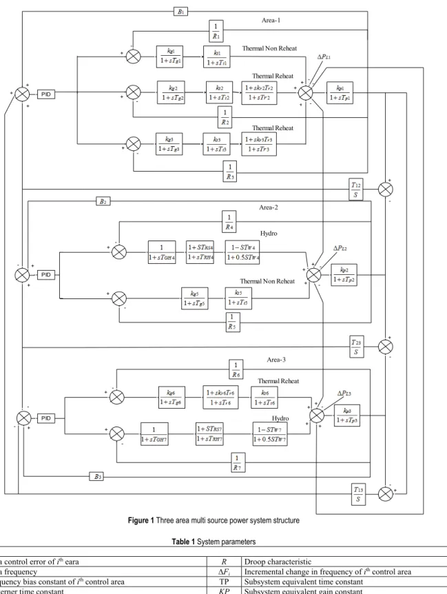
A three-area power system as shown in Fig. 1 is considered to evaluate the proposed method. Different generation sources are used in each area. Area 1 includes thermal non-reheat and reheat generators, while areas 2 and 3 include hydro and thermal reheat. System parameters are defined in Tab. 1. The connection between different areas is shown in Fig. 1. The dynamic models of generators used in the simulations are explained in [16-18].

As occurrence of any disturbance in each area causes frequency changes in all areas and tie line power deviation from scheduled values. A PID controller is used in each area in order to quickly damp oscillations and to reduce the overshoot and undershoot values. DE algorithm is used to optimize the parameters. Controller input is ACE signal. ACE

is a linear combination of tie line power frequency that can be defined for each area i'th as Eq. (1).

,

i tie ij i i

j

ACE =

∑

∆P + ∆β f (1) In Eq. (1), ΔPtie,ij is the power exchange between areas i

and j, βi is basic frequency coefficient of area i and Δfi is

frequency deviation of area i. In a multi-area power system,

Tijis considered as synchronizing coefficient between areas i

and j, and Δpiis also considered as load disturbances in area

i.

3 DESIGN OF CONTROLLER

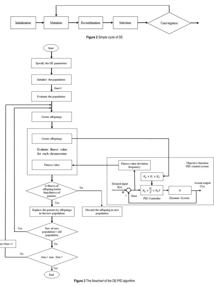
Differential Evolution (DE) technique is a population-based heuristic optimization algorithm [14-15]. Benefits of DE are: Simpleness, efficiency, and real coding. Generally, the base of DE is Genetic Algorithm (GA). However, unlike simple GA that uses binary coding for representing problem parameters, DE uses real coding of floating point numbers. The crucial idea behind DE is a scheme for generating trial parameter vectors. Basically, DE works with two populations; old generation and new generation of the same population. It works through a simple cycle of stages as Fig. 2.

Stage 1: Initial Population

A population of fixed size to generated where each variable has its lower and upper bounds.

Stage 2: Mutation

Selection of vectors to a base individual in order to explore the search space.

1 1 1( 2 3 ) iG r G r G r G V + = X +F X −X (2) 1 1( 2 3 ) iG bestG r G r G V + =X +F X −X (3) 1 1 1( 2 3 ) 2( 1 ) iG r G r G r G bestG r G V + = X +F X −X +F X −X (4)

Where: i = 1,…, NP; r1, r2, r3∈ {1,…, NP} are randomly selected and satisfy; r1≠ r2≠ r3≠ i; F ∈ [0, 1], F is the control parameter/mutation factor proposed by Storn and Price [3].

Stage 3: Recombination or crossover

Mix successful solutions from the previous generation with current donors. The perturbed individual, ViG+1 = (v1,iG+1,…, vn,iG+1) and the current population member, ViG = (x1,iG,…,

xn,iG) are subject to the crossover operation, which finally

generates the population of candidates, or "trial" vectors,

UiG+1 = (u1,iG+1,…, un,iG+1) as follows: , 1 , , 1 , if or otherwise i jG i j rand i jG i jG V rand CR j I U X + + ≤ =  =   (5)

With randi,j ~ U(0, 1), Irand is a random integer from (1,

2,…, D) where D is the solution’s dimension, i.e. number of control variables and CR ∈ [0, 1].

Stage 4: Selection

To keep the population size constant over subsequent generations, selection operation is performed. In this operation the target vector XiG is compared with the trial

vector ViG+1 and the one with the better fitness value is

admitted to the next generation. The selection operation in DE can be represented by:

1 1 1 iG _otherwise if ( iG ) ( iG) iG iG V F U F X X X + + + <  =   (6)

Proportional integral derivative controller (PID) is one of the most popular feedback controllers in the process industries because of its stability and fast response.

Design of PID controller requires determination of the three main parameters, Proportional gain Kp, Integral gain Ki

and Derivative gain Kd. The integral square error (ISE)

criterion is considered as the objective function for the present work which is described in Eq. (7).

2 2

0 ( )d

tsim

tie

ISE=

_∫

∆ + ∆f P t (7)

Where Δf is the system frequency deviation in area-i and area-j, respectively, 2

tie P

∆ is the incremental change in tie line power and tsim is the time range of simulation. Fig. 3 shows

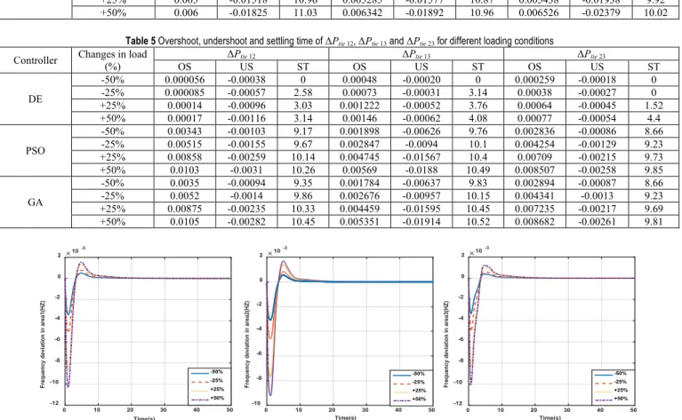
flowchart of proposed DE and PID controller. The problem constraints are the controller parameter bounds. Therefore, the design problem can be formulated as the following optimization problem.

Minimum ISE. Subject to:

Kp min≤ Kp≤ Kp max, Ki min≤ Ki≤ Ki max and Kd min≤ Kd≤

Kd max. Kmin, Kmax are the minimum and maximum value of

the control parameters. The flowchart of the DE-PID algorithm is shown Fig. (3).

4 THE SIMULATION RESULTS

An interconnected power system includes three-area power system as shown in Fig. 1, which is simulated in Sim/Matlab software. System parameters have been defined according to the Tab. 1 and their values are shown in Tab. 2.

(3)

Power required in each area is considered to be ΔpL = 0.1 pu

MW. PID controller is used in each area for automatic generation control. The controller parameters are optimized using DE, PSO, and GA algorithms.

Figure 1 Three area multi source power system structure Table 1 System parameters

Nomenclature

ACEi Area control error of ith eara R Droop characteristic

F Area frequency ∆Fi Incremental change in frequency of ith control area

Bi Frequency bias constant of ith control area TP Subsystem equivalent time constant

Tg Governer time constant KP Subsystem equivalent gain constant

Tt Turbine time constant Tij Synchronizing coefficient between area i and j

Tr System turbine reheat time constant epfk Economic participation factor of kth generation unit

TGH Hydro turbine speed governer main servo time constant cpfk Constant participation factor between kth_{GENCO and}_ith_DISCO

TRS Hydro turbine speed governer reset time ∆Ptie,ij Scheduled power tie line power flow between area i and j TRH Hydro turbine speed governer transient droop time constant ∆PDi Total power control and uncontrolled for DISCO area ith

TW Nominal starting time of water in penstock ∆Pgk Power output of kth generating unit

PID PID PID ++ + - -+ + + -+ + + + -+ -+ -+ -+ -+ -+ -+ -+ + + + + -+ -+ -+ -+ Area-1 Thermal Non Reheat

Thermal Reheat

Area-2 Hydro

Thermal Non Reheat

Area-3 Thermal Reheat

(4)

Figure 2 Simple cycle of DE

Figure 3 The flowchart of the DE-PID algorithm Figs. 4 and 5 show the dynamic response of the system

frequency deviation and tie-line power exchange between different areas respectively, in present of DE, PSO and GA

algorithms. From Figs. 4 and 5 it is clear that overshoot and undershoot is minimal.

(5)

Figure 4 Dynamic response of the system frequency deviation

Figure 5 Dynamic response of tie line power deviation Table 2 Power system parameter values

Area 1: Area 2: Area 3:

Tg1 = 0.08 s Tt1 = 0.35 s 1 0.3333 MWHz_pu R = kg1 = 1 kt1 = 1 Tg2 = 0.875 s Tt2 = 0.375 s kr2 = 0.3113 Tr2 = 10.6 s 2 0.32 MWHz_pu R = kg2 = kt2 = 1 Tg3 = 0.08 s Tt3 = 0.3 s kr3 = 0.5 Tr3 = 10 s 3 0.33 MWHz_pu R = kg3 = kt3 = 1 1 20 MWHz_pu p k = Tp1 = 120 s 1 0.532 Hz_MWpu B = f = 60 Hz TGH4 = 0.1 s TRH4 = 10 s TRS4 = 0.513 s TW4 = 1 s 4 0.32 MWHz_pu R = kg4 = kt4 = 1 Tg5 = 0.075 s Tt5 = 0.38 s 5 0.2963 MWHz_pu R = kg5 = kt5 = 1 2 20 MWHz_pu p k = Tp2 = 120 s 1 0.495 Hz_MWpu B = f = 60 Hz Tg6 = 0.07 s Tt6 = 0.36 s Kr6 = 0.33 Tr6 = 10 s 6 0.289 MWHz_pu R = kg6 = kt6 = 1 TGH7 = 0.015 s TRH7 = 8.75 s TRS7 = 0.1513 s TW7 = 1.5 s 7 0.3077 MWHz_pu R = kg7 = kt7 = 1 3 20 MWHz_pu p k = Tp3 = 120 s 3 0.542 Hz_MWpu B = f = 60 Hz T12 = T23 = T13 = 0.543 pu/H

Tab. 3 shows the amount of overshoot, undershoot and settling time in exchange of power system all three algorithms. The results show that the dynamic performance of DE algorithm is suitable.

4.1 Controller Performance against Load Changes

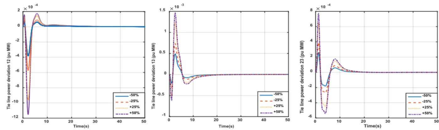
In order to evaluate the performance of the controller against possible load variation, the load of all areas changes from −50% to +50%. Figs. 6 and 7 show the frequency deviation and tie-line power exchange between different areas respectively. The amount of overshoot, undershoot and settling time in various states of load changes for three algorithms is shown in Tabs. 4 and 5.

Results in Tabs. 4 and 5 clearly show that increment in rate of load, increases the measured values and the DE algorithm has more satisfactory performance in the case of load changes. The effect of reducing the amount of load up to −50%, settling time for the tie-line power exchange between different areas will be zero.

This shows that the controller proposed is well managed from the beginning and control deviations without any delay within the desired precision and show satisfactory performance. In the case of load reduction up to −25%, the settling time for Δptie23 also has a similar situation.

Time(s)

0 10 20 30 40 50

Frequency deviation in area1(HZ)

10-3 -15 -10 -5 0 5

DE tuned PID controller pso tuned PID controller GA tuned PID controller

Time(s)

0 10 20 30 40 50

10-3 -15 -10 -5 0 5

Time(s)

0 10 20 30 40 50

Frequency Deviation in area3(HZ)

10-3 -20 -15 -10 -5 0 5

Time(s)

0 10 20 30 40 50

Tie line power deviation 12 (pu MW)

10-3 -4 -2 0 2 4 6 8

Time(s)

0 10 20 30 40 50

10-3 -14 -12 -10 -8 -6 -4 -2 0 2 4

Time(s)

0 10 20 30 40 50

10-3 -2 -1 0 1 2 3 4 5

6 _{DE tuned PID controller}

pso tuned PID controller GA tuned PID controller

(6)

Table 3 Overshoot, undershoot and settling time for base case with PID controller using DE, PSO and GA algorithms GA PSO DE Parameters _OS _US _ST _OS _US _ST _OS _US _ST 10.82 -0.0121 0.004 10.79 -0.0122 0.0041 6.96 -0.0068 0.00102 Δf1 10.75 -0.0126 0.0042 10.75 -0.0124 0.00415 7.209 -0.00614 0.00115 Δf2 9.8 -0.0158 0.0043 9.84 -0.0157 0.0043 7.09 -0.0067 0.000818 Δf2 10.16 -0.00188 0.007 9.95 -0.00207 0.0068 2.83 -0.00077 0.000113 ΔPtie 12 10.35 -0.0127 0.00356 10.28 -0.0125 0.0037 3.44 -0.00041 0.00097 ΔPtie 13 9.51 -0.00174 0.00578 9.523 -0.00172 0.00567 1.35 -0.00036 0.00051 ΔPtie 23

Table 4 Overshoot, undershoot and settling time of Δf1, Δf2, Δf3 for different loading conditions

Δf3 Δf2 Δf1 Changes in load (%) Controller _OS _US _ST _OS _US _ST _OS _US _ST 3.17 -0.0033 0.000409 5.67 -0.00307 0.000574 5.23 -0.0034 0.00051 -50% DE _+25%-25% 0.00076 _0.00128 -0.00515 _-0.0085 _7.436.37 0.00086 _0.00143 -0.0046 _-0.0076 6.63 _7.61 0.00061 _0.00102 -0.00502 _-0.0083 6.37 _7.54 8.01 -0.01005 0.00122 7.92 -0.00921 0.00172 7.83 -0.0103 0.00154 +50% 9.33 -0.00789 0.00219 10.2 -0.00621 0.00207 10.28 -0.0061 0.00206 -50% PSO _+25%-25% 0.00309 _0.0051 -0.00924 _-0.01541 _10.9310.6 _0.0051960.00311 -0.00932 _-0.0155 10.53 _10.87 _0.0054750.00328 -0.01184 _-0.01973 9.62 _9.95 10.05 -0.02368 0.00657 10.96 -0.01865 0.006236 11.03 -0.01849 0.00617 +50% 9.36 -0.00793 0.002175 10.24 -0.0063 0.00211 10.33 -0.00608 0.002 -50% GA _+25%-25% 0.003 _0.005 _-0.01518-0.0091 10.65 _10.96 _0.0052850.00317 _-0.01577-0.0094 10.57 _10.87 0.003263 _0.005438 _-0.01938-0.0119 9.65 _9.92 10.02 -0.02379 0.006526 10.96 -0.01892 0.006342 11.03 -0.01825 0.006 +50%

Table 5 Overshoot, undershoot and settling time of ΔPtie 12, ΔPtie 13and ΔPtie 23 for different loading conditions

ΔPtie 23 ΔPtie 13 ΔPtie 12 Changes in load (%) Controller _OS _US _ST _OS _US _ST _OS _US _ST 0 -0.00018 0.000259 0 -0.00020 0.00048 0 -0.00038 0.000056 -50% DE _+25%-25% 0.000085 _0.00014 -0.00057 _-0.00096 _3.032.58 _0.0012220.00073 -0.00031 _-0.00052 3.14 _3.76 0.00038 _0.00064 -0.00027 _-0.00045 _1.520 4.4 -0.00054 0.00077 4.08 -0.00062 0.00146 3.14 -0.00116 0.00017 +50% 8.66 -0.00086 0.002836 9.76 -0.00626 0.001898 9.17 -0.00103 0.00343 -50% PSO _+25%-25% 0.00515 _0.00858 -0.00155 _-0.00259 _10.149.67 0.002847 _0.004745 _-0.01567-0.0094 10.1 _10.4 0.004254 _0.00709 -0.00129 _-0.00215 9.23 _9.73 9.85 -0.00258 0.008507 10.49 -0.0188 0.00569 10.26 -0.0031 0.0103 +50% 8.66 -0.00087 0.002894 9.83 -0.00637 0.001784 9.35 -0.00094 0.0035 -50% GA _+25%-25% _0.008750.0052 _-0.00235-0.0014 _10.339.86 0.002676 _0.004459 -0.00957 _-0.01595 10.15 _10.45 0.004341 _0.007235 _-0.00217-0.0013 9.23 _9.69 9.81 -0.00261 0.008682 10.52 -0.01914 0.005351 10.45 -0.00282 0.0105 +50%

Figure 6 System response of frequency deviation for different loading changes

4.2 Evaluation of Controller against Changes in System Parameters

In order to further evaluate the performance of the proposed controller under various conditions, several system parameters such as Tt(turbine time constant), Tr (reheat time

constant), TGH (hydro turbine speed governor main servo

time constant), TRS (hydro turbine speed governer reset

time), TRH (hydro turbine speed governer transient droop

time constant) have been changed in the range of −25% to +25% compared to their nominal values by considering the coefficients of an optimal controller.

Important dynamic indices are overshoot, undershoot and settling time which are measured and tabulated in Tabs. 6 and 7. The results show that the values of the indices measured are in an acceptable range and close to the values of the parameters of the system.

Time(s)

0 10 20 30 40 50

10-3 -12 -10 -8 -6 -4 -2 0 2 -50% -25% +25% +50% Time(s) 0 10 20 30 40 50

10-3 -10 -8 -6 -4 -2 0 2 -50% -25% +25% +50% Time(s) 0 10 20 30 40 50

10-3 -12 -10 -8 -6 -4 -2 0 2 -50% -25% +25% +50%

(7)

Figure 7 System response of tie-line power deviation for different loading changes

Table 6 Overshoot, undershoot and setting time of Δf1, Δf2, Δf3 for different values of system parameters

Δf3 Δf2 Δf1 Changes in load (%) System parameters OS US ST OS US ST OS US ST 7.3 -0.0059 0.00081 7.46 -0.0057 0.00108 7.3 -0.00629 0.00099 -25% Tt _+25% _0.0011 _-0.0074 _6.3 _0.00147 _-0.00659 _7.61 _0.00156 _-0.0075 _7.21 6.94 -0.00659 0.0008 7.03 -0.00611 0.00117 6.65 -0.0068 0.001 -25% Tr _+25% _0.00102 _-0.0069 _7.14 _0.00113 _-0.00616 _7.31 _-0.0082 _-0.0067 _7,17 7.07 -0.0067 0.00081 7.19 -0.00612 0.00114 6.93 -0.00688 0.00102 -25% TGH _+25% _0.00103 _-0.0068 _6.99 _0.00115 _-0.0061 _7.22 _0.00082 _-0.0066 _7.11 7.15 -0.0066 0.00085 7.23 -0.00617 0.00116 7.03 -0.00682 0.00104 -25% TRS _+25% _0.0010 _-0.0069 _6.89 _0.00113 _-0.00611 _7.18 _0.00077 _-0.0067 _7.01 7.20 -0.0073 0.00113 6.43 -0.0063 0.00126 6.38 -0.00707 0.00106 -25% TRH _+25% _0.00090 _-0.00677 _7.31 _0.00105 _-0.00606 _7.51 _0.00082 _-0.0063 _7.28

Table 7 Overshoot, undershoot and setting time of ΔPtie 12, ΔPtie 13and ΔPtie 23 for different values of system parameters

ΔPtie 23 ΔPtie 13 ΔPtie 12 Changes in load (%) System parameters OS US ST OS US ST OS US ST 0 -0.00039 0.00043 3.93 -0.00027 0.00070 2.57 -0.00055 8.01×10−5 -25% Tt _+25% _0.00028 _-0.00109 _2.89 _0.00154 _-0.00058 _3.1 _0.00062 _-0.00051 _2.66 0 -0.00039 0.00046 3.30 -0.00037 0.00112 2.80 -0.00083 0.000175 -25% Tr _+25% _0.000105 _-0.000726 _2.89 _0.00088 _-0.00044 _3.53 _0.00055 _-0.00033 _1.46 1.36 -0.00036 0.00052 3.44 -0.00042 0.00098 2.85 -0.00078 0.000116 -25% TGH _+25% _0.0001107 _-0.000763 _2.86 _0.00097 _-0.00041 _3.47 _0.00051 _-0.00035 _1.31 1.31 -0.00038 0.00051 3.59 -0.00037 0.00092 2.82 -0.000689 9.47×10−5 -25% TRS _+25% _0.000144 _-0.000859 _2.89 _0.00104 _-0.00046 _3.32 _0.00053 _-0.00036 _1.35 2.75 -0.00055 0.00066 3.44 -0.00077 0.00180 3.27 -0.00126 0.0002521 -25% TRH _+25% _0.000113 _-0.00064 _2.41 _0.00066 _-0.00025 _2.94 _0.00045 _-0.00038 ₀ 5 CONCLUSION

In this paper, the design of an intelligent controller in interconnected large power system has been presented. An extensive analysis of proposed LFC system controller in the interconnected power system has been done when execution of the changes load demand and changes in system parameters are taken into account. Results clearly show that PID controller reaches to zero deviations in steady state in frequency and tie line power quickly.

In order to show superiority of PID designed controller using DE algorithm, the results of the Differential Evolution technique of parameters such as frequency and power tie line changes compared with the results of the PSO and GA algorithms. Results prove that DE algorithm has better overshoot, undershoot and settling time in all possible as compared to PSO and GA. Furthermore, the results of simulations show that the proposed algorithm is not affected by changes in load and uncertainty in the system parameters and the controller has satisfactory dynamic operation.

6 REFERENCES

[1] Prakash, S. & Sinha, S. (2014). Simulation based neuro-fuzzy hybrid intelligent PI control approach in four-area load frequency control of interconnected power system. Applied Soft Computing, 23, 152-164.

https://doi.org/10.1016/j.asoc.2014.05.020

[2] Padhan, D. G. & Majhi, S. (2013). A new control scheme for PID load frequency controller of single-area and multi-area power systems. ISA transactions, 52(2), 242-251.

https://doi.org/10.1016/j.isatra.2012.10.003

[3] Sahu, R. K., Panda, S., & Rout, U. K. (2013). DE optimized parallel 2-DOF PID controller for load frequency control of power system with governor dead-band nonlinearity. International Journal of Electrical Power & Energy Systems, 49, 19-33. https://doi.org/10.1016/j.ijepes.2012.12.009

[4] Chandrakala, K. V. & Balamurugan, S. (2016). Simulated annealing based optimal frequency and terminal voltage control of multi source multi area system. International Journal of Electrical Power & Energy Systems, 78, 823-829. https://doi.org/10.1016/j.ijepes.2015.12.026

[5] Anwar, M. N. & Pan, S. (2015). A new PID load frequency controller design method in frequency domain through direct

Time(s)

0 10 20 30 40 50

10-4 -12 -10 -8 -6 -4 -2 0 2 -50% -25% +25% +50% Time(s) 0 10 20 30 40 50

10-3 -1 -0.5 0 0.5 1 1.5 -50% -25% +25% +50% Time(s) 0 10 20 30 40 50

10-4 -6 -4 -2 0 2 4 6 8 -50% -25% +25% +50%

(8)

synthesis approach. International Journal of Electrical Power & Energy Systems, 67, 560-569.

https://doi.org/10.1016/j.ijepes.2014.12.024

[6] Nikmanesh, E., Hariri, O., Shams, H., & Fasihozaman, M. (2016). Pareto design of load frequency control for interconnected power systems based on multi-objective uniform diversity genetic algorithm (muga). International Journal of Electrical Power & Energy Systems, 80, 333-346. https://doi.org/10.1016/j.ijepes.2016.01.042

[7] Hota, P. & Mohanty, B. (2016). Automatic generation control of multi source power generation under deregulated environment. International Journal of Electrical Power & Energy Systems, 75, 205-214.

[8] Khooban, M. H. & Niknam, T. (2015). A new intelligent online fuzzy tuning approach for multi-area load frequency control: Self Adaptive Modified Bat Algorithm. International Journal of Electrical Power & Energy Systems, 71, 254-261.

[9] Yesil, E. (2014). Interval type-2 fuzzy PID load frequency controller using Big Bang–Big Crunch optimization. Applied Soft Computing, 15, 100-112.

https://doi.org/10.1016/j.asoc.2013.10.031

[10] Mosaad, M. I. & Salem, F. (2014). LFC based adaptive PID controller using ANN and ANFIS techniques. Journal of Electrical Systems and Information Technology, 1(3), 212-222. https://doi.org/10.1016/j.jesit.2014.12.004

[11] Nayak, J. R., Pati, T. K., Sahu, B. K., & Kar, S. K. (2015). Fuzzy-PID controller optimized TLBO algorithm on automatic generation control of a two-area interconnected power system. Paper presented at the Circuit, Power and Computing Technologies (ICCPCT 2015), International Conference on. https://doi.org/10.1109/ICCPCT.2015.7159427

[12] Sekhar, G. C., Sahu, R. K., Baliarsingh, A., & Panda, S. (2016). Load frequency control of power system under deregulated environment using optimal firefly algorithm. International Journal of Electrical Power & Energy Systems, 74, 195-211. https://doi.org/10.1016/j.ijepes.2015.07.025

[13] Dhillon, S. S., Lather, J. S., & Marwaha, S. (2015). Multi area load frequency control using particle swarm optimization and fuzzy rules. Procedia Computer Science, 57, 460-472. https://doi.org/10.1016/j.procs.2015.07.363

[14] Sahu, R. K., Sekhar, G. C., & Panda, S. (2015). DE optimized fuzzy PID controller with derivative filter for LFC of multi source power system in deregulated environment. Ain Shams Engineering Journal, 6(2), 511-530.

https://doi.org/10.1016/j.asej.2014.12.009

[15] Rocca, P., Oliveri, G., & Massa, A. (2011). Differential evolution as applied to electromagnetics. IEEE Antennas and Propagation Magazine, 53(1), 38-49.

https://doi.org/10.1109/MAP.2011.5773566

[16] Parmar, K. S., Majhi, S., & Kothari, D. (2012). Load frequency control of a realistic power system with multi-source power generation. International Journal of Electrical Power & Energy Systems, 42(1), 426-433.

[17] Report, I. (1973). Dynamic models for steam and hydro turbines in power system studies. IEEE Transactions on Power Apparatus and Systems (6), 1904-1915.

https://doi.org/10.1109/TPAS.1973.293570

[18] De Mello, F. & Ahner, D. (1994). Dynamic models for combined cycle plants in power system studies. IEEE Transactions on Power Systems, 9(3).

https://doi.org/10.1109/59.336085

Authors’ contacts:

Alireza SINA, Faculty member of ACECR, Research scholar in UIET Panjab University,

Sector 14, Chandigarh, Punjab 160014, India [email protected]

Damanjeet KAUR, Assistant Professor of Electrical & Electronics Engineering, UIET Panjab University,

Sector 14, Chandigarh, Punjab 160014, India [email protected]