Page 1 of 148
Development and evaluation of ADME models using
proprietary and opensource data
By
Maria-Anna Trapotsi
July 2017
A thesis submitted to the University of Hertfordshire in partial fulfilment of the requirements for the degree of Master of Science by Research
Page 2 of 148 Abstract
Absorption, Distribution, Metabolism and Elimination (ADME) properties are important factors in the drug discovery pipeline. Literature ADME data are often collected in large chemical databases like ChEMBL, which might be an asset to improve the prediction of ADME properties. Pharmaceutical companies build ADME Quantitative Structure Property Relationships (QSPR) models using proprietary data and thus the inclusion of literature data might be a valuable source for the development of predictive models. The aim of this study was to investigate whether merging literature and proprietary data could improve the predictive activity of proprietary models and enlarge their applicability domain (AD).
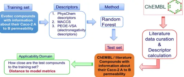
ADME predictive models for Caco-2 (A to B) permeability and LogD7.4 were built with data extracted from Evotec and ChEMBL database. Predictive models were developed for each property and three different training sets were used based on: proprietary compounds (Evotec models), literature compounds (ChEMBL models) and a merged set of proprietary and literature compounds (Evotec+ChEMBL models). The Random Forest (RF), Partial Least Squares (PLS) and Support Vector Regression (SVR) were used to develop the models. The performance of the models was evaluated by using two types of test sets: a diverse test set (20 % compounds of available data randomly selected) and a temporal test set (data published after the models were built). The descriptors that used were the physiochemical descriptors, the structural Molecular Access System (MACCS) descriptors and the Partial equalisation of orbital electronegativity – van der Walls surface areas (Peoe-VSA) descriptors. The AD of the models was evaluated with four distance to model metrics, which were the: kNN with Euclidean distance, kNN with Manhattan distance, Leverage and Mahalanobis distance.
The ability of an existing Evotec Caco-2 permeability model to assess literature compounds (extracted from ChEMBL) was evaluated. The literature test set was predicted with a higher RMSE compared to the RMSE in prediction for internal compounds. Additionally, a number of literature compounds was found to be outside the AD of the Evotec model, thus highlighting an area of improvement for proprietary Evotec models. Furthermore, the effect of the inclusion of literature data in the existing Caco-2 permeability and LogD7.4 Evotec proprietary models was evaluated. The RF algorithm was the highest performing method for the development of Caco-2 permeability models and the SVR for the LogD7.4 models. In addition, the leverage method proved to be the most appropriate for the evaluation of the models’ AD. The permeability model built merging literature and proprietary data (Evotec+ChEMBL model) predicted a literature temporal test set with an RMSE of 0.68 while the Evotec model showed an RMSE of 0.74. Even in the case of the Evotec temporal test set, the two models performed similarly and the AD of the mixed models (incorporating both literature and proprietary data) was enlarged. The 86.15% of the compounds in the proprietary temporal test set were within the AD of the Evotec+ChEMBL model, while 76.50% of the compounds of the same test set appeared to be within the AD of the Evotec model. Similarly, the LogD7.4 Evotec+ChEMBL model predicted a literature temporal test set with an RMSE of 0.77 while the Evotec model showed an RMSE of 0.83. Even in the case of the Evotec temporal test set, the two models performed similarly but the AD of the mixed models (incorporating both literature and
Page 3 of 148
proprietary data) was enlarged. The 94.86% of the compounds in the proprietary temporal test set were within the AD of the Evotec+ChEMBL model, while 88.49% of the compounds of the same test set appeared to be within the AD of the Evotec model.
This study demonstrated that the inclusion of public ADME data into proprietary models improved the performance of proprietary models and enlarged at the same time their AD. The methodology presented herein will be applied by Evotec computational scientists to re-build the Caco-2 and LogD7.4 Evotec proprietary models considering literature data as discussed in this thesis.
Page 4 of 148 Acknowledgments
I would like to thank my academic supervisor Professor Mire Zloh from the University of Hertfordshire and my industrial placement supervisors, Dr Mirco Meniconi and Dr Mike Bodkin from Evotec for their help, advice and support throughout this project. I would also like to thank Dr Patrick Barton form the Evotec DMPK department for the help and support throughout this project.
I would also like to thank the Research Informatics group at Evotec that made me feel welcome and part of the group.
Finally, I would like to thank my family for the encouragement and support throughout my studies.
Page 5 of 148 Table of Contents Abstract ... 2 Acknowledgments ... 4 List of Figures ... 8 List of Tables ... 11 1 INTRODUCTION... 14
1.1 ADME properties in drug development process... 14
1.2 QSAR and QSPR modelling ... 15
1.3 Data collection and curation ... 16
1.3.1 Literature data and databases for ADME data collection for QSPR modelling 16 1.4 Calculation of molecular descriptors ... 17
1.5 Feature Selection ... 18
1.6 Model Building and Machine learning in QSPR model development ... 19
1.6.1 Multiple Linear Regression (MLR) ... 20
1.6.2 Partial Least Squares (PLS) ... 21
1.6.3 Decision Trees (DTs) and Random Forest (RF) in machine learning ... 21
1.6.4 Support Vector Machines (SVM) ... 23
1.6.5 Konstanz Information Miner (KNIME) in QSPR model building ... 26
1.7 Model Validation ... 26
1.7.1 Applicability domain (AD) ... 27
1.7.1.1 Distance to model metrics ... 27
1.7.1.2 Mahalanobis distance ... 28
1.7.1.3 Leverage ... 28
1.7.1.4 Other Distances ... 29
1.7.2 k-Nearest Neighbour (kNN) ... 29
1.7.3 Fingerprints and Similarity measures used with kNN ... 30
1.8 Principal Component Analysis (PCA) ... 30
1.9 Permeability ... 31
1.9.1 Structure of the cell membrane and Drug Transport ... 32
1.9.2 In-vitro models of cell permeability ... 33
1.9.3 In-silico regression permeability models developed with Caco-2 data ... 35
Page 6 of 148
1.10.1 Theoretical lipophilicity prediction and the importance in-silico lipophilicity models 39
1.11 Research Hypothesis and Aims ... 42
2 MATERIALS AND METHODS... 43
2.1 Software Framework ... 43
2.2 Methods used for the evaluation of existing Evotec Caco-2 A to B permeability model with literature data ... 43
2.2.1 Literature data curation ... 44
2.2.2 Standardisation and Molecular descriptors calculation ... 45
2.2.3 Prediction of Caco-2 permeability of compounds downloaded from ChEMBL by Evotec existing model ... 48
2.2.4 Model Performance ... 48
2.2.5 Metrics to establish the Applicability Domain ... 48
2.2.5.1 Principal Component Analysis and Stopping Rule ... 48
2.2.5.2 Evaluation of AD with Distance to model metrics ... 49
2.2.5.3 Distance to model metrics and thresholds ... 50
2.2.6 Statistical Analysis ... 51
2.3 Overview of methods used for the Development of in-silico predictive models .. 51
2.3.1 Literature data curation for the development of in-silico Caco-2 permeability and LogD7.4 models ... 53
2.3.2 Selection of training and test sets ... 54
2.3.2.1 Subsequent model assessment for Caco-2 permeability models ... 57
2.3.3 Standardisation of Molecular descriptors ... 58
2.3.4 Algorithms and their parameter optimisation for model building ... 58
2.3.4.1 Random Forest (RF) parameter selection ... 58
2.3.4.2 Partial Least Squares (PLS) parameter selection ... 59
2.3.4.3 Support Vector Regression (SVR) parameter selection ... 59
2.3.5 Estimation of the AD of the in-silico Caco-2 permeability and LogD7.4 models with distance to model metrics ... 60
3 RESULTS AND DISCUSSION ... 61
3.1 Evaluation of existing Evotec Caco-2 A to B permeability model with opensource data 61 3.1.1 Model Assessment ... 61
Page 7 of 148
3.1.3 Evaluation of distance to model metrics ... 64
3.1.3.1 Bin compounds by distance ... 65
3.1.3.2 Bin compounds by squared residuals ... 69
3.1.3.3 Group compounds based on distance threshold ... 72
3.1.3.4 kNN with Tanimoto and Dice ... 74
3.1.4 Conclusion ... 75
3.2 Evaluation of Caco-2 in-silico permeability models ... 76
3.2.1 Models developed with literature data (ChEMBL models) ... 76
3.2.2 Models developed with proprietary data (Evotec models) ... 79
3.2.3 Models developed with merged proprietary and literature data (Evotec+ChEMBL models) ... 82
3.2.4 Comparison of Caco-2 permeability models with models reported in the literature ... 84
3.2.5 The effect of merging proprietary and literature data in the development of Caco-2 permeability models ... 88
3.2.6 Subsequent model assessment of the Caco-2 permeability models ... 93
3.2.7 Applicability Domain estimation of the in-silico Caco-2 permeability models ... 94
3.3 Evaluation of in-silico LogD7.4 models. ... 98
3.3.1 Models developed with literature data (ChEMBL models) ... 98
3.3.2 Models developed with proprietary data (Evotec models) ... 102
3.3.3 Models developed with proprietary and literature data (Evotec+ChEMBL models) 104 3.3.4 Comparison of LogD7.4 models with models reported in the literature ... 107
3.3.5 The effect of merging proprietary and literature data in the development of LogD7.4 models ... 112
3.3.6 Applicability Domain estimation of the in-silico LogD7.4 models ... 115
4 CONCLUSION AND FUTURE WORK ... 119
4.1 Conclusions ... 119
4.2 Future work ... 122
5 REFERENCES ... 124
Page 8 of 148 List of Figures
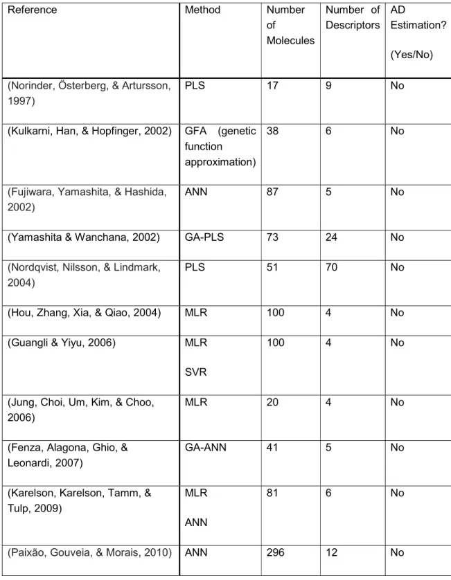
Figure 1: Computer Aided Drug Design (CADD) in drug design and development process (adapted from Kore, Mutha, Antre, Oswal, & Kshirsagar, 2012). ... 15 Figure 2: The steps of the QSPR development process (adapted from Cherkasov et al., 2014). ... 16 Figure 3: Summary of the QSAR or QSPR building methods (adapted from Dudek, Arodz and Gálvez, 2006; Danielle, 2014). ... 20 Figure 4: Schematic representation of a decision tree (adapted from Dehmer et al, 2012). . 22 Figure 5: Schematic representation of two data classes in a 2D space by the SVM algorithm. ... 25 Figure 6: Illustration of the lipid bilayer and the structural unit of the lipid bilayer, the
phospholipids. ... 32 Figure 7: A simplified view of the two main permeability mechanisms. ... 33 Figure 8: Biopharmaceutics Classification System (BCS)(adapted from Benet, 2013) ... 34 Figure 9: Schematic representation of the Caco-2 permeability assay (adapted from Li, 2001). ... 34 Figure 10: Schematic summary of the work and the methods used for the evaluation of the existing Evotec Caco-2 A to B permeability model. ... 43 Figure 11: Schematic representation of the literature data filtering process for the compounds downloaded from ChEMBL. The arrow indicates the flow of the process. ... 44 Figure 12: An example of different forms that a chemical can be represented (ChemAxon, 2016a) ... 45 Figure 13: KNIME workflow for the calculation of descriptors: a) overall descriptor calculation workflow, b) physiochemical descriptors, c) MACCS keys and d) Peoe-VSA. ... 47 Figure 14: Screenshot of the workflow that was created for the PCA and the estimation of the AD with the four different distance to model metrics in the descriptor space. ... 50 Figure 15: Overview of the workflow that was created for the PCA and the estimation of the AD with the four different distance to model metrics in the chemical space. ... 50 Figure 16: Overview of the methodology process followed for the development of in-silico
Caco-2 A to B permeability and LogD7.4 predictive models... 52 Figure 17: Schematic representation of the literature data filtering process for the compounds downloaded from ChEMBL for the development of in-silico Caco-2 permeability and LogD7.4 models. The arrow indicates the flow of the process. ... 53 Figure 18: Schematic representation of the distances of the test set compounds from the training sets. The arrows indicate the distances that were calculated. ... 60 Figure 19: Experimental values for Caco-2 permeability of ChEMBL compounds vs the predicted Caco-2 permeability obtained with Evotec Caco-2 model. ... 61
Page 9 of 148
Figure 20: Principal component plot of Principal Component 1 vs Principal Component 2 for Evotec (blue) and ChEMBL (red) compounds. Figures in brackets indicate the percentage of variance explained by the corresponding PC. ... 63 Figure 21: Scree plot of the eigenvalues from the Evotec compounds PCA (blue) and the eigenvalues obtained from the Avg-R on Evotec compounds PCA (orange). ... 64 Figure 22: RMSE in prediction of the binned a) Euclidean distance to 5NNs, b) Manhattan distance to 5NNs, c) Leverages and d) Mahalanobis Distance for CHEMBL compounds calculated with the descriptors. ... 66 Figure 23: RMSE in prediction of the binned a) Euclidean distance to 5NNs, b) Manhattan distance to 5NNs, c) Leverages and d) Mahalanobis Distance for CHEMBL compounds calculated with the first 27 PCs. ... 67 Figure 24: Average a) Euclidean distance to 5NNs, b) Manhattan distance to 5NNs,
Leverages and d) Mahalanobis Distance of the binned squared residuals for CHEMBL compounds calculated with the descriptors. ... 70 Figure 25: Average a) Euclidean distance to 5NNs, b) Manhattan distance to 5NNs,
Leverages and d) Mahalanobis Distance of the binned squared residuals for CHEMBL compounds calculated with the 27 first PCs. ... 71 Figure 26: RMSE in prediction of the binned similarity to 5NNs for CHEMBL compounds calculated with: a) Tanimoto and b) Dice coefficients in ECFP4 fingerprint space. ... 74 Figure 27: Experimental versus predicted Caco-2 permeability of compounds in the ChEMBL diverse test set obtained with the ChEMBL model developed with the SVR algorithm. Caco-2 permeability is reported as Log10 (A->B Papp[10-6 cm/s]). The black solid line represents the line of best fit in the form of y=b+ax. The red and dark blue dashed lines represent the y=x±1 and the y=x±0.5 respectively. ... 78 Figure 28: Experimental versus predicted Caco-2 permeability of compounds in the ChEMBL temporal test set obtained with the ChEMBL model developed with SVR algorithm. Caco-2 permeability is reported as Log10 (A->B Papp[10-6 cm/s]). The black solid line represents the line of best fit in the form of y=b+ax. The red and dark blue dashed lines represent the y=x±1 and the y=x±0.5 respectively. ... 78 Figure 29: Experimental versus predicted Caco-2 permeability of compounds in the Evotec diverse test set obtained with the Evotec model developed with RF algorithm. Caco-2 permeability is reported as Log10 (A->B Papp[10-6 cm/s]). The black solid line represents the line of best fit in the form of y=b+ax. The red and dark blue dashed lines represent the y=x±1 and the y=x±0.5 respectively... 80 Figure 30: Experimental versus predicted Caco-2 permeability of compounds in the Evotec temporal test set obtained with the Evotec model developed with RF algorithm. Caco-2 permeability is reported as Log10 (A->B Papp[10-6 cm/s]). The black solid line represents the line of best fit in the form of y=b+ax. The red and dark blue dashed lines represent the y=x±1 and the y=x±0.5 respectively... 81
Page 10 of 148
Figure 31: Experimental versus predicted Caco-2 permeability of compounds in the
Evotec+ChEMBL diverse test set obtained with the Evotec+ChEMBL model developed with RF algorithm. Caco-2 permeability is reported as Log10 (A->B Papp[10-6 cm/s]). The black solid line represents the line of best fit in the form of y=b+ax. The red and dark blue dashed lines represent the y=x±1 and the y=x±0.5 respectively. ... 83 Figure 32: Experimental versus predicted Caco-2 permeability of compounds in the
Evotec+ChEMBL temporal test set obtained with the Evotec+ChEMBL model developed with RF algorithm. Caco-2 permeability is reported as Log10 (A->B Papp[10-6 cm/s]). The black solid line represents the line of best fit in the form of y=b+ax. The red and dark blue dashed lines represent the y=x±1 and the y=x±0.5 respectively. ... 83 Figure 33: Experimental versus predicted logD7.4 values of compounds in the ChEMBL diverse test set obtained with the ChEMBL model developed with the SVR algorithm. LogD7.4 lipophilicity is reported as Log10 D. The black solid line represents the line of best fit in the form of y=b+ax. The red and dark blue dashed lines represent the y=x±1 and the y=x±0.5 respectively. ... 100 Figure 34: Experimental versus predicted logD7.4 values of compounds in the ChEMBL temporal test set obtained with the ChEMBL model developed with the SVR algorithm. LogD7.4 lipophilicity is reported as Log10 D. The black solid line represents the line of best fit in the form of y=b+ax. The red and dark blue dashed lines represent the y=x±1 and the y=x±0.5 respectively. ... 100 Figure 35: Experimental versus predicted logD7.4 values of compounds in the Evotec diverse test set obtained with the Evotec model developed with the SVR algorithm. LogD7.4
lipophilicity is reported as Log10 D. The black solid line represents the line of best fit in the form of y=b+ax. The red and dark blue dashed lines represent the y=x±1 and the y=x±0.5 respectively. ... 103 Figure 36: Experimental versus predicted logD7.4 values of compounds in the Evotec
temporal test set obtained with the Evotec model developed with the SVR algorithm. LogD7.4 lipophilicity is reported as Log10 D. The black solid line represents the line of best fit in the form of y=b+ax. The red and dark blue dashed lines represent the y=x±1 and the y=x±0.5 respectively. ... 103 Figure 37: Experimental versus predicted logD7.4 lipophilicity of compounds in the
Evotec+ChEMBL diverse test set obtained with the Evotec+ChEMBL model developed with the SVR algorithm. LogD7.4 lipophilicity is reported as Log10 D. The black solid line represents the line of best fit in the form of y=b+ax. The red and dark blue dashed lines represent the y=x±1 and the y=x±0.5 respectively. ... 106 Figure 38: Experimental versus predicted LogD7.4 lipophilicity of compounds in the
Evotec+ChEMBL temporal test set obtained with the Evotec+ChEMBL model developed with the SVR algorithm. LogD7.4 lipophilicity is reported as Log10 D. The black solid line represents the line of best fit in the form of y=b+ax. The red and dark blue dashed lines represent the y=x±1 and the y=x±0.5 respectively. ... 106
Page 11 of 148 List of Tables
Table 1: Regression permeability models developed with Caco-2 data reported in the
literature during 1997-2010. ... 36 Table 2: Regression permeability models developed with Caco-2 data reported in the
literature during 2016-2017. ... 38 Table 3: Regression lipophilicity models developed with logD7.4 data reported in the literature. ... 41 Table 4: Training and Temporal test sets used in development of the in-silico permeability models. ... 55 Table 5: Training and Diverse test sets used in development of the in-silico permeability models. ... 55 Table 6: Training and Temporal test sets used in development of the in-silico LogD7.4 models. ... 56 Table 7: Training and Diverse test sets used in development of the in-silico LogD7.4 models. ... 56 Table 8: Training and temporal test sets new temporal test sets used in the subsequent models assessment for the in-silico permeability models. ... 57 Table 9: Summary of the Distance to model metrics. ... 65 Table 10: Statistical analysis of the RMSE of the bins (data are binned by distance). ... 69 Table 11: Statistical analysis of the average distance of the bins (data are binned by squared residuals). ... 72 Table 12: The table depicts the percentage of the compounds and the RMSE for the
compounds inside and outside of the AD. The Mann Whitney results and the number of descriptors or PCs used are also shown. ... 73 Table 13: RMSE in prediction and R2 of ChEMBL diverse test set and ChEMBL temporal test set obtained with the ChEMBL model by using three different machine learning methods (RF, PLS &SVR). The red colour indicates the model that produced the lower RMSE in each testing strategy. ... 77 Table 14: RMSE in prediction and R2 of Evotec diverse test set and Evotec temporal test set obtained with the Evotec model by using three different machine learning methods (RF, PLS &SVR). The red colour indicates the model that produced the lower RMSE in each testing strategy. ... 80 Table 15: RMSE in prediction and R2 of Evotec+ChEMBL diverse test set and
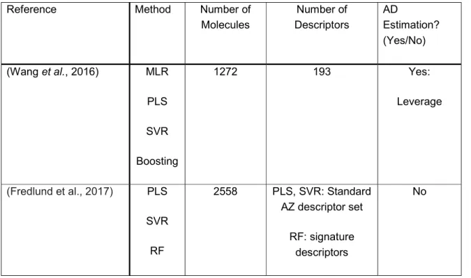
Evotec+ChEMBL temporal test set obtained with the Evotec+ChEMBL model by using three different machine learning methods (RF, PLS &SVR). The red colour indicates the model that produced the lower RMSE in each testing strategy. ... 82 Table 16: The two most recent regression permeability models developed with caco-2 data. ... 85
Page 12 of 148
Table 17: RMSE in prediction and R2 of: literature ChEMBL model by Wang et al (2016), ChEMBL model, Evotec models and Evotec+ChEMBL model on their diverse test sets. The red colour indicates the highest performing modelling algorithm for each model. ... 86 Table 18: RMSE in prediction of Boosting model developed by Wang et al (2016) and of the new model developed with Wang et al (2016) training and test sets with present study’s methodology. The red colour indicates the highest performing model. ... 87 Table 19: Table shows the model performance of “ChEMBL”, “Evotec” and
“Evotec+ChEMBL” models. The RMSE in prediction and R2 of Evotec and ChEMBL diverse test sets are reported. Results obtained by applying the RF, PLS and SVR algorithms. The red colour indicates the highest performing model between the Evotec and Evotec+ChEMBL models. ... 90 Table 20: Table shows the model performance of “ChEMBL”, “Evotec” and
“Evotec+ChEMBL” models. The RMSE in prediction and R2 of Evotec and ChEMBL temporal test sets are reported Results obtained by applying the RF, PLS and SVR algorithms. The red colour indicates the highest performing model between the Evotec and Evotec+ChEMBL models. ... 90 Table 21: Table shows the model performance of the “initial” (M1) and “new” (M2)
“ChEMBL”, “Evotec” and “Evotec+ChEMBL” models. The RMSE in prediction of the “new” Evotec and ChEMBL temporal test sets is reported. Results obtained by applying the RF algorithm and the red colour indicates the highest performing model between Evotec and Evotec+ChEMBL models. ... 93 Table 22: Results obtained with the kNN with Euclidean distance, kNN with Manhattan distance, Leverage and Mahalanobis distance for the three different Caco-2 permeability models and the two different temporal test sets. The table summarises: the percentage of compounds inside the AD of the models, the RMSE in prediction of compounds inside and outside the AD and the assessment of the statistical significance with the Mann Whitney (MW) test. The red colour indicates the presence of a statistically significant difference in the RMSE of the compounds inside and outside of the AD. ... 95 Table 23: RMSE in prediction and R2 of ChEMBL diverse test set and ChEMBL temporal test set obtained with the ChEMBL model by using three different machine learning methods (RF, PLS &SVR). The red colour indicates the model that produced the lower RMSE in each testing strategy. ... 99 Table 24: RMSE in prediction and R2 of Evotec diverse test set and Evotec temporal test set obtained with the Evotec model by using three different machine learning methods (RF, PLS &SVR). The red colour indicates the model that produced the lower RMSE in each testing strategy. ... 102 Table 25: RMSE in prediction and R2 of Evotec+ChEMBL diverse test set and
Evotec+ChEMBL temporal test set using different machine learning methods (RF, PLS &SVR). The red colour indicates the model that produced the lower RMSE in each testing strategy. ... 105
Page 13 of 148
Table 26: Regression lipophilicity models developed with logD7.4 data reported in the
literature. ... 108 Table 27: Model assessment results of SVR models developed by Wang et al (2015) and of the new models developed with Wang et al (2015) training and test set and the present study’s methodology (descriptors and algorithms). ... 110 Table 28: RMSE in prediction and R2 of ChEMBL and Evotec diverse test sets and ChEMBL and Evotec temporal test set. Results obtained by using the ChemAxon software, and the ChEMBL, Evotec and Evotec+Chembl models developed with the SVR algorithm. ... 111 Table 29: Table shows the model performance of “ChEMBL”, “Evotec” and
“Evotec+ChEMBL” models. The RMSE in prediction and R2 of Evotec and ChEMBL diverse test sets are reported. Results obtained by applying the RF, PLS and SVR algorithms. The red colour indicates the highest performing model between the Evotec and Evotec+ChEMBL models. ... 113 Table 30: Table shows the model performance of “ChEMBL”, “Evotec” and
“Evotec+ChEMBL” models. The RMSE in prediction and R2 of Evotec and ChEMBL temporal test sets are reported. Results obtained by applying the RF, PLS and SVR algorithms. The red colour indicates the highest performing model between the Evotec and Evotec+ChEMBL models. ... 113 Table 31: Results obtained with the kNN with Euclidean distance, kNN with Manhattan distance, Leverage and Mahalanobis distance to model metrics for the three different LogD7.4 models and the two different temporal test sets. The table summarises: the percentage of compounds inside the AD of the models, the RMSE in prediction of compounds inside and outside the AD and the assessment of the statistical significance with the Mann Whitney (MW) test. The red colour indicates the presence of a statistically significant difference in the RMSE of the compounds inside and outside of the AD. ... 116
Page 14 of 148 1 INTRODUCTION
1.1 ADME properties in drug development process
The pharmaceutical drug design and development process is time consuming, complex and characterised by high risk and cost (Wang & Urban, 2004). It has been estimated that the probability of success in Phase II clinical trials is only 34 % (Cumming, Davis, Muresan,
Haeberlein, & Chen, 2013). The efficacy and ADME (Absorption, Distribution, Metabolism,
Elimination) properties play a significant role in the drug mechanism (Thompson, 2000) and are considered as an integral part of the drug design process (Di & Kerns, 2016).
A molecule should be able to exhibit both a pharmacological effect and also to have the appropriate ADME properties to reach the market as a drug. Or in other words, a drug should not only be efficacious for the target disease but also with an acceptable pharmacokinetic and safety profile (Davies et al., 2015). Some of these parameters include the lipophilicity, ionisation, solubility and molecular mass (Livingstone & Davis, 2012). For example, a highly lipophilic drug can be more permeable (i.e. greater absorption) (Riley, Parker, Trigg, & Manners, 2001), can undergo greater metabolic clearance (Patrick, 2013) and it can be better absorbed in the GI tract (Avdeef & Tam, 2010). In addition, lipophilicity can affect the ability of a drug to cross the Blood Brain Barrier (BBB) and the volume of distribution (Poulin & Theil, 2002) because of the drug ability to bind to serum albumin (Patrick, 2013). As a result, parameters such as lipophilicity should be taken into account from the early stages of drug design in order to exclude compounds with unwanted properties.
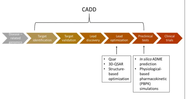
The total loss rate due to poor ADME properties was near 50% in 2004 (Khanna, 2012). Although the failure rate was reduced to 14% (Tsaioun, 2007) due to the preclinical testing, there is a potential to improve cost-effectiveness of the drug discovery and development by using predictive ADME predictive models. Therefore, it is of major significance for pharmaceutical industries to improve the productivity of the drug design process (Paul et al., 2010) and reduce failure due to poor ADME properties. Computational chemistry can be a great asset in drug discovery process (Liao, Sitzmann, Pugliese, & Nicklaus, 2011), as its application can reduce the risk and cost of the drug design process (Tan et al., 2010). A useful tool of the computational medicinal chemistry is the in-silico predictive ADME models. The great advantage of these models is the prediction of a molecule’s ADME properties (Zhang, Luo, Ding, & Lu, 2012) prior to chemical synthesis and in-vitro or in-vivo testing, which will save time and money (Zhang & Surapaneni, 2012) in preclinical testing (figure 1). Therefore, the number of compounds that have to be synthesised to obtain the required biochemical and physicochemical profile is reduced (Moroy, Martiny, Vayer, Villoutreix, & Miteva, 2012).
Page 15 of 148
Figure 1: Computer Aided Drug Design (CADD) in drug design and development process (adapted from Kore, Mutha, Antre, Oswal, & Kshirsagar, 2012).
1.2 QSAR and QSPR modelling
Quantitative Structure Activity Relationship (QSAR) and Quantitative Structure Property Relationship (QSPR) modelling are major and commonly employed computational tools in medicinal chemistry to help the lead optimization process in drug discovery (Cramer, 2012; Kore et al., 2012). QSAR is widely used to provide optimisation of the pharmacological activity, and QSPR can provide information about pharmacokinetic or ADME properties (Puzyn, Leszczynski, & Cronin, 2010). QSPR models are mathematical models, which relate the chemical structure of the compound to a physiochemical property and this relation can be used to predict ADME properties (Yee & Wei, 2012). QSPR modelling can provide exploration and exploitation of the relationship between the chemical structure of the compounds and their ADME properties (Tropsha, 2010) prior to the synthesis of a compound (Park et al., 2014). The introduction of QSAR/QSPR models, has raised concerns for the predictability and applicability of these models (Jaworska, Nikolova-Jeliazkova, & Aldenberg, 2005). Therefore, five
principles have been established for QSAR/QSPR model validation: 1. a defined endpoint, 2.
an unambiguous algorithm, 3. a defined domain of applicability, 4. appropriate measures of goodness-of-fit, robustness and predictivity and 5. a mechanistic interpretation, if possible
(Sahigara et al., 2012). One of the most important principles is the applicability domain, which
Page 16 of 148
Figure 2: The steps of the QSPR development process (adapted from Cherkasov et al., 2014). 1.3 Data collection and curation
Figure 2 is schematically depicting the process of building a QSPR. The first step of that process involves the data collection and curation. This is a significant part of the QSPR development because the performance of the model depends on the quality of the training set (Yee & Wei, 2012). Literature data and databases can be considered as an increasingly important source for collection of compounds and these data have been used for the development of QSPR models (Wang, Cao, Zhu, & Yun, 2015; Wang et al., 2016).
1.3.1 Literature data and databases for ADME data collection for QSPR modelling Literature data are published in journal articles (peer-reviewed or scientific) and thus it is usually difficult to manually search and extract information. For example, literature chemical structures are usually depicted as images and that is making the extraction and use of literature data in QSPR development difficult (Gaulton et al., 2012). Therefore, in the recent years a variety of publicly available databases have been developed due to the high demand for easy, free and open access to the literature information. As a result, the construction of QSPR models is greatly assisted by the development of large publicly available compound databases like PubChem BioAssay (Li, Cheng, Wang, & Bryant, 2010; Y. Wang et al., 2010), ChemBank (Seiler et al., 2008), ZINC (Irwin, Sterling, Mysinger, Bolstad, & Coleman, 2012), ochem.eu (online chemical database with modelling environment) (Wang et al., 2016) and ChEMBL (Bento et al., 2014; Gaulton et al., 2012).
The three databases that store information for ADME assays are the PubChem BioAssay, ochem.eu and ChEMBL. The other databases like ZINC is used mainly for ligand discovery (Irwin et al., 2012) and ChemBank has been developed to guide chemists in the synthesis of
Data Collection and Curation
Calculation of Molecular Descriptors
Feature Selection
ADME Model Building
Page 17 of 148
novel compounds and biologists to search for small molecules that catalyse a specific process (Seiler et al., 2008). ChEMBL is the database, which is considered as a key representative of the current plethora of publicly available data (which also include the majority of the information available in PubChem BioAssay and ochem.eu) (Papadatos & Overington, 2014; Wang et al., 2009) and has dramatically changed the way that the drug discovery community shares and deposits experimental data. Moreover, CHEMBL extracts the information from the medicinal chemistry literature (Papadatos, Gaulton, Hersey, & Overington, 2015), mainly from 12 prominent chemistry journals (Bender, 2010). Moreover, companies like AstraZeneca deposited compounds into ChEMBL (Clark et al., 2015).
ChEMBL contains information obtained by various assays, which are divided into four categories: 1. Binding (B), Functional (F), Toxicity (T) and ADME (A) and additionally include annotations related to the relevant assays. This is a great advantage of ChEMBL, which other databases lack. These supplementary annotations are useful and help the data curation process but the level of detail of annotations is not always sufficient to truly identify the protocols of the ADME assays (Papadatos et al., 2015). Even when the assay conditions seem to be the same, a significant variability is observed between measurements by different laboratories (Kalliokoski et al., 2013). Therefore, ChEMBL team has set future plans to improve the quality and consistency of the data by including more detailed description of the assays’ parameters (Papadatos et al., 2015). One of the main disadvantages in ChEMBL is the quality and reliability of the literature sources. For example, an error in chemical structure might result into an erroneous descriptor calculation (Tropsha, 2010), which will ultimately affect the predictability of the model. Manual curation of the data downloaded from public databases can substantially improve the accuracy of prediction (Young, Martin, Venkatapathy, & Harten, 2008). The error in commercial or public databases ranges from 0.1% - 3.4% (Fourches, Muratov, & Tropsha, 2010) and another example is that of WOMBAT (world of molecular bioactivity) database with an overall error rate of 8% (Young et al., 2008). Therefore, it is important to curate the data extracted from large chemical databases before the development of the models.
1.4 Calculation of molecular descriptors
After the first step in QSPR process, which is the data collection and curation (figure 2), the next step is the calculation of molecular descriptors. Molecular descriptors are a basic tool for cheminformatics, which is used to transform chemical information (like physiochemical properties) into a numerical data and they can be theoretically (derived from symbolic molecule representation) or experimentally derived (Puzyn, Leszczynski and Cronin, 2010).
Topological descriptors are widely used for QSPR modelling and they refer to 2D molecular descriptors (Rajkhowa & Deka, 2014), which are based on the distances between atoms calculated by the number of intervening bonds (Puzyn et al., 2010) and thus considering the internal arrangement of compound’s atoms (Pillai, 2015). Therefore, topological descriptors can give numerical information about molecular size, presence of heteroatoms, multiple bonds (Gozalbes & Doucet, 2002) and enable for the identification of the individual atoms and the
Page 18 of 148
bonded connections between them (Roy, Kar, & Das, 2015). The Molecular Access System or “MACCS keys” is considered as the best known and the prototype of key-based fingerprints (Chackalamannil, Rotella, & Ward, 2017). MACCS are structural descriptors and are based on pattern matching of the chemical structure of a compound to a pre-defined set of structural fragments, (166 MACCS keys) (Wale, Watson, & Karypis, 2008). Another set of descriptors that can be used are the partial equalization of orbital electronegativity - van der Walls surface areas (Peoe-VSA) descriptors, which capture the direct electrostatic interactions (Bajorath, 2004). For example, electrostatic interactions play a role in the metabolism and protein binding, because these interactions can affect the binding of a compound to the active site of the metabolic enzyme and the plasma proteins (Cyprotex, 2015).
Other important 2D descriptors that can be used for ADME models are Polar Surface Area (PSA), number of hydrogen bond acceptors/donors, LogP, LogD at various pH (which can be either experimentally or theoretically calculated) and pKa (Hou, Li, Zhang, & Wang, 2009). For example, the H bonding behaviour of a compound can be useful for the description of drug permeability because as the number of hydrogen bonds increases, the polarity of the compound increases too and the lipophilicity becomes weaker. As a result the compound is less able to cross the cell membrane by passive diffusion (Wang et al., 2016) because hydrogen bonds are formed with the outer phase of the membrane. In addition, PSA is one of the most significant molecular descriptors in QSPR studies and is a measure of polarity of the compound, which indicates the presence of a dipole moment (Caron & Ermondi, 2016). PSA is an area of Van der Waals surface, which results from oxygen, nitrogen or hydrogen atoms bound to polar areas (Danielle, 2014). As a result, PSA is related to the hydrophobicity and polarity of a molecule and is useful in estimating the compound’s absorption, BBB permeability and other ADME characteristics (Kubinyi, Folkers, & Mannhold, 2008). For example, PSA should be low (60-70Å2) for BBB penetration and no more than 140 Å2 for cell membrane permeation (Pajouhesh & Lenz, 2005) and generally PSA gives excellent correlation with drug permeability in Caco-2 monolayers (Artursson, Palm, & Luthman, 2012).
In addition to the 2D QSAR descriptors, there also the 3D descriptors for QSAR modelling (3D QSAR) like randic molecular profiles, geometrical descriptors etc. One of the most widely used 3D QSAR method is the Comparative Molecular Field Analysis (CoMFA), which concerns mainly the electrostatic field and steric relationships between the ligand and biological target (Cherkasov et al., 2014). However, it is considered as a computationally intense process (Goodarzi & Dejaegher, 2012) and one example might be the conformational analysis to find the best conformer.
1.5 Feature Selection
A feature selection or variable selection is usually performed to choose the descriptors with goal to reduce the dimensionality and the redundancy of the descriptors that are chosen. Feature selection usually depends on two parameters. The first is the correlation and variance of descriptors and the second is the algorithm that is applied to the training set. Correlated descriptors are those which are different views of the same molecular aspect (Puzyn et al.,
Page 19 of 148
2010). Therefore, some algorithms like MLR cannot produce meaningful results with correlated descriptors, whereas other methods like PLS and SVR can handle sets that contain correlated descriptors. In addition, zero or very low variance descriptors can be removed. They do not carry any information because they are constant for all the chemical compounds. There are various methods to perform feature/variable selection and they are categorised into three groups: filters, wrappers and embedded methods. The filter methods use a metric or score for each feature, based on a statistical measure and based on their score are excluded or included (Brownlee, 2016). An example of a filter method is the ReliefF, which randomly picks dataset points and finds their nearest neighbours. Then it assigns weight to the features/descriptors based on how good they can discriminate the observations from their neighbours (Eklund, Norinder, Boyer, & Carlsson, 2014). The wrapper methods use a learning algorithm and identify descriptors subsets. Models are developed and assess which descriptor combinations can result in a good model accuracy (Brownlee, 2016). The embedded methods incorporate the feature selection during the application of learning algorithm (Eklund et al., 2014). However, it was shown that the use of different feature selection methods did not improve the prediction accuracy of models developed with “state-of-the-art” algorithms (RF, ANN, SVM) (Eklund et al., 2014). The reason is that these algorithms can handle correlated descriptors. 1.6 Model Building and Machine learning in QSPR model development
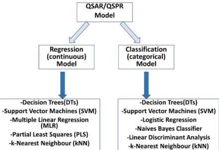
One of the most significant factor in QSPR building process is the selection of an appropriate method. QSPR models have evolved significantly since scientists decided to utilise approaches from recent developments in other fields like data mining, pattern recognition, machine learning and artificial intelligence (Dudek, Arodz, & Gálvez, 2006; Geppert, Vogt, & Bajorath, 2010). Various algorithms are used to identify patterns and correlations within a dataset/training set, and through data mining process, a model is derived (Lavecchia, 2015). Each compound is considered as a vector and each molecular descriptor corresponds to 1 dimension/variable. The resulting model relates a set of descriptors with biologically relevant properties like lipophilicity and other parameters, which can affect ADME properties. There are various types of models and they are usually divided into two broad categories: continuous (regression) and classification (categorical) (Dudek, Arodz, & Gálvez, 2006) (figure 3).
Page 20 of 148
Figure 3: Summary of the QSAR or QSPR building methods (adapted from Dudek, Arodz and Gálvez, 2006; Danielle, 2014).
1.6.1 Multiple Linear Regression (MLR)
MLR is a supervised machine learning method that is able to establish a linear mathematical relationship between a property of the training compounds and a set of descriptors that encode the chemical information (Ventura, Latino, & Martins, 2013). MLR is a commonly used method for constructing QSPR models (Liu & Long, 2009) and the prediction is derived as a linear function of all descriptors (Sethi, 2012). The following equation gives the linear relationship between the target value and the compounds’ features/descriptors:
= + + + ⋯ + (Equation 1),
where n is the number of descriptors, x1, x2, …, xn are the molecular descriptors, β1, β2, ..., βn are descriptors’ coefficients and β0 is the model constant
Equation 1 represents a hyperplane in a space of n-dimensions. In addition, the coefficients of that equation are calculated with methods like the least-squares method, which minimizes the sum of squared residuals (Dehmer, Varmuza, & Bonchev, 2012). However, there are disadvantages related to MLR. For example correlated descriptors and a large descriptors to compounds number ratio are two factors that MLR cannot handle and result in unstable predictions (Dudek, Arodz & Gálvez, 2006). The underlying reason is that descriptors influence the calculation of the coefficients and therefore correlated descriptors could result in erroneous estimation. Additionally, the number of compounds should be at least five times the number of descriptors to reduce the possibility of erroneous coefficient calculation.
Page 21 of 148 1.6.2 Partial Least Squares (PLS)
PLS is a more popular method compared to MLR because it overcomes the disadvantages of MLR mentioned above. PLS uses similar principles with Principal Component Analysis (PCA) and it is suitable to overcome the issues related to the multicollinearity and the high ratio of the number of descriptors over the number of compounds (Dudek, Arodz & Gálvez, 2006). PLS is able to project the original variables (i.e. descriptors) into latent variables (LVs) and thus reducing the dimensionality (Xing et al., 2014). LVs do not only explain the variation in the x variables (descriptors) as the PCA does. They also take into account how the variation in the x variables corresponds to the variation of the dependent variable y (target value) (Brown, 2015). The following equations correspond to the latent variables (LVi), which are linear combinations of the variables/ descriptors (xi).
= + + ⋯ + (Equation 2), where y is the target value, α is the regression coefficient and LV are the latent variables
in a chemical space with n descriptors/dimensions = . + . + ⋯ + . = . + . + ⋯ + . . . . = . + . + ⋯ + . (Equation 3), where LV are the latent variables, i the number of the LVs, b are the variable coefficients,
x are the molecular descriptors and n the number of descriptors.
Each LV (equation 3) is a linear combination of the x values and also their corresponding coefficient (b), which gives an approximation to the variation of the target value (y) (Leach & Gillet, 2007). This method decomposes the input matrix of descriptors into loadings and LVs and the later are orthogonal and are capturing the descriptor information (Sethi, 2012). 1.6.3 Decision Trees (DTs) and Random Forest (RF) in machine learning
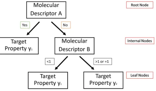
Decision Trees (DTs) are algorithms that are used for both regression and classification models and thus they are usually referred as Classification And Regression Trees (CART) (Brownlee, 2016). The DTs are predictive models that map observations to target values (Lodhi, 2010). DTs as every machine learning algorithm has an input and output. In ADME predictive modelling, the aim is to develop a model that can predict the value of a target (e.g. permeability, lipophilicity, protein binding etc.) based on a set of input variables (descriptors) (Tsaioun & Kates, 2011). The input data are in the form of (x, y) = [(x , x , … , x ), y], where n is the number of descriptors and y represents the target value. In a DT, there are three types of nodes: a root node, internal nodes, and leaf nodes. Leaf nodes are also known as terminal nodes. An example of how a DT works is shown in figure 4. It is an example of a classification problem and thus the DT classifies the compounds on target property y1 or y2. The
Page 22 of 148
classification of the test compounds is based on the leaf/terminal node that they reach after going through a series of questions (Yee & Wei, 2012). For example, according to the DT shown in figure 4, a test compound will be assigned with the y1 if it displays a certain condition for molecular descriptor A. If it does not fulfil that condition, then the molecular Descriptor B is examined. If the molecular descriptor B has a value less than 1, then the test compound will be assigned with the target property y1 or if it has a value greater or equal to 1, then the test compound will be assigned with the target property y2.
Figure 4: Schematic representation of a decision tree (adapted from Dehmer et al, 2012). As the example above shows, a DT works by systematically subdividing the information within a training data (in the root and internal nodes) based on rules and there are various algorithms to define these rules (Dehmer et al., 2012). One of them is the recursive binary splitting (Brownlee, 2016). According to that algorithm, different split points are tried and evaluated with a cost function. The cost function that is used for regression models is expressing the sum squared residuals and is the following:
∑ ( − ) (Equation 4), where i is the number of compounds and y the experimental value
The output of this algorithm represents the assignment of y value of each leaf for the test set compounds. However, this procedure provides a greedy approach because at each step a split point is defined, which might be good for that specific step but not for the overall of the DT. This limitation of the DTs can be overcome with the use of ensembles DTs like Random Forest (RF).
Page 23 of 148
RF is based on an ensemble of DTs (Mitchell, 2014; K. Roy et al., 2015), which are built by training data of multiple features. Ensemble is the procedure that combines the results/predictions from multiple predictive algorithms in order to make a more accurate prediction compared to each individual prediction (Brownlee, 2016), as it benefits from the “wisdom of crowds” effect (Mitchell, 2014). RF is an improvement of the DTs because the learning algorithm is limited to a random sample compared to DTs, which are searching all the data to identify the ideal split point based on the minimisation of the sum of the squared residuals. The data are partitioned into progressively increasing homogeneous group through the tree. As a result, each terminal node of the DTs is comprised by molecules, which exhibit a similar value of the ADME property evaluated (Mitchell, 2014). RF is generally a unique combination of prediction accuracy, model interpretability and it is able to handle missing values and a variety of variables (binary, continuous, categorical) (Qi, 2012). RF can be used to perform both classification and regression models (Bajorath et al., 2012; Oprea, 2006) and the choice depends on the property that is predicted. Therefore, it is increasingly used in the field of biological computational sciences (Yang, Yang, Zhou & Zomaya, 2010). RF is an algorithm used in the literature to develop ADME predictive models like lipophilicity (Rodgers, Davis, Tomkinson, & van de Waterbeemd, 2011; Schroeter et al, 2007; Wang et al., 2015), permeability (Fredlund, Winiwarter, & Hilgendorf, 2017) and solubility (Palmer, O’Boyle, Glen, & Mitchell, 2006). The main disadvantage of RF method is that its performance can be influenced by a small sample size and also by the number of trees selected (Dehmer et al., 2012). The selection of optimal parameters can be achieved through cross validation (Statnikov, Wang, & Aliferis, 2008).
1.6.4 Support Vector Machines (SVM)
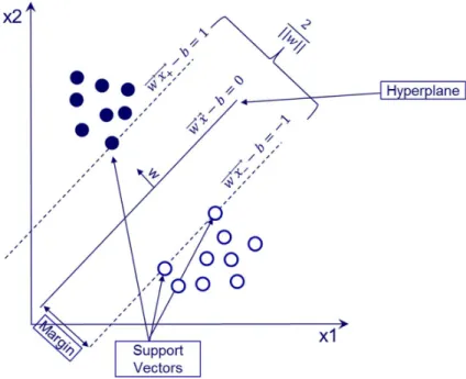
The SVM is an algorithm developed by Vapnik and co-workers and it is a widely used algorithm in the field of data mining in cheminformatics. It can be used for both classification and regression problems and when it is used for continuous/regression models can be referred as Support Vector Regression (SVR). It is an algorithm extensively used to predict properties like hERG blockade (Doddareddy, Klaasse, & IJzerman, 2010; Li, Jørgensen, Oprea, & Brunak, 2008), toxicity related properties (Mitchell, 2014), protein inhibition (Dong et al., 2009) etc. It has also been used to predict physiochemical properties like LogD7.4 (Schroeter et al., 2007; Wang et al., 2015), melting point (Hughes, Palmer, & Nigsch, 2008) and pKa (Harding & Wedge, 2009). For example, for a two class classifier in a 2D space, where the data are linearly separable, the SVM algorithm aims to find the maximum margin hyperplane that divides the data in a way that all the data with target value +1 lie on the opposite site from those with target value -1 (Basak, Pal, & Patranabis, 2007). This hyperplane is also referred as separate hyperplane and the margin is the distance between the separating hyperplane and data samples that are closest to that hyperplane and are called support vectors (Raschka, 2015) (figure 5). Therefore, the SVM for a classification problem aims to identify the optimal hyperplane for which the margin of separation between the chemical compounds is maximised (Khan, 2012). If w is a normal vector to the hyperplane then the hyperplane equation can be written as:
Page 24 of 148 − = 0 (Equation 5)
and the equations of the two parallel hyperplanes can be written as:
+ − = 1 (Equation 6), − = −1 (Equation 7).
As the w vector is perpendicular to the hyperplane it is also perpendicular to the parallel hyperplanes and therefore the vector from the x(-) to x(+) is scalar multiple (r) of the vector w and the following equation can be written:
= + r (Equation 8).
By using equation 6 and substitute equation 8 to the x(+), the equation 9 is obtained: (Eq.6)( . ) ( + ) − = 1 ⇒ ⇒ + | | − = 1 ⇒ ⇒ − + | | = 1 ⇒ ⇒ −1 + | | = 1 ⇒ ⇒ | | = 2 ⇒ ⇒ = 2/ | | (Equation 9)
The Margin (M) is the half of the distance between x(-) and x(+). Therefore: 2 = | − | = | | ( .5)
⇒ | | = 2
| |2 | | ⇒ ⇒ 2M = 2
| | ( 10)
Page 25 of 148
Figure 5: Schematic representation of two data classes in a 2D space by the SVM algorithm. The case outlined above is the simplest case, where the data are linearly separable in a 2D space and can be easily schematically represented. In more complicated cases, where the data i) are not linearly separable, ii) exist in a higher dimensional space and iii) the aim is the development of a regression model, there are additional strategies to follow. In the non-linearly separable cases, the data are projected in a higher dimension space with the aim to be able to linearly separate them. The kernel trick is used to map the training set data into a higher dimensional space with a mapping function (Φ) (Khan, 2012). There are various kernels that could be used and one of the most widely used is the radial basis function (rbf) kernel ( ( , )) for two samples/vectors , of the input space (Raschka, 2015). The rbf kernel can be expressed as the inner product of the projected , and uses the following equation to map the data in a higher dimension:
( , ) = ∑(( ) ) (Equation 11), where , are two vectors of the input space and γ is a hyperparameter.
To train the data with the SVM algorithm and the rbf as a kernel, three hyperparameters (ε, γ and C) should be optimised. The ε parameter is affecting the number of support vectors and it can have a value in the range of 0-1. The larger the ε value is, the lower is the number of support vectors (Khan, 2012). The γ parameter is also taking values in the range of 0-1 and the usual default value is 0.1. If the γ increases, the influence of each data sample is also increased (Raschka, 2015). The C parameter is one of the most important parameter because it can affect both the trained and predicted data (Wang et al., 2015). The C value represents a
Page 26 of 148
balance between the margin maximisation and the training error minimisation (Khan, 2012). If the C is too large then the SVM algorithm will produce an overfitted model (Brownlee, 2016) and if it is too small, insufficient stress is introduced on fitting the training data (Khan, 2012; Wang et al., 2015). A grid search is usually used to find an optimal combination for the three hyperparameters described above.
1.6.5 Konstanz Information Miner (KNIME) in QSPR model building
Literature databases have significantly increased the availability and accessibility of data (Schadt, Linderman, Sorenson, Lee, & Nolan, 2010) and as a result there is a high demand of data mining tools that respond to these needs. KNIME is a data mining workflow framework, which has significantly evolved to meet the new demands of automating predictions and machine learning. It is a pipeline package, which provides a user friendly workspace (Mazanetz, Marmon, Reisser, & Morao, 2012). It uses nodes for data input and various nodes are interconnected to create a pipeline, where information is flowing through them (a process known as “visual programming”). This software offers the advantage of preparing workflows, which can be quickly customised to manage data and information in order to automatize tasks
(Mazanetz et al., 2012). KNIME is used in both academia and industry and special nodes have
been designed for the KNIME software, which can be used in chemistry, biology and in drug design process. For example, two cheminformatics node packages that are widely used for the development of ADME models are the: ChemAxon/Infocom Marvin package and the Weka (Waikato Environment for Knowledge Analysis). Other examples of package nodes, which are developed from the KNIME community contributions are: Enalos (Melagraki, Afantitis, Sarimveis, & Koutentis, 2009; Melagraki & Afantitis, 2013) and RD-kit, Chemical Development
Kit (CDK) (Mazanetz et al., 2012). The KNIME software is coded in Java based on an Eclipse
environment (Warr, 2012) and thus it is an extensible programme through plug-ins, which offers additional functionality (Berthold et al., 2009). KNIME also offers nodes, which are serving as interfaces for statistic/mathematic programmes (Matlab, R), programme languages (Python) and database readers (Jagla, Wiswedel, & Coppée, 2011). Finally, KNIME can be used in the development of ADME models because data mining and specialised KNIME nodes can be used for the development of predictive models.
1.7 Model Validation
Model validation is a very important process that should be performed after the model training. Model validation can be internal or external (Chackalamannil et al., 2017). An example of internal validation is the k-fold cross-validation, which partitions the initial dataset in k samples. Then a subsample is excluded and a model is built with the k-1 subsamples as training set. This procedure is repeated for k times and every subsample has been used once as the validation test set (Alpaydin, 2014). Moreover, an external validation set should also be used because it investigates the generalisability of the model to predict new chemicals (Puzyn et al., 2010). There are also measures that estimate the goodness-of-fit of the model. Two of the most commonly used are the Root Mean Square Error (RMSE) in prediction and the Pearson Correlation coefficient or the coefficient of variation in the fit to training set (R2)
Page 27 of 148
(Chackalamannil et al., 2017). The RMSE is a useful measure as it has the same units as the units in the QSPR experiment and provides indication of the likely error associated with the model’s predictions. The RMSE (equation 12) is generally used as a statistical metric to establish model performance (Chai & Draxler, 2014) and the lower the values of RMSE the higher the accuracy of the model. The R2 (equation 13) is often used to measure model quality (Wermuth, 2008). According to Wermuth (2008) the R2 can be misleading because it depends heavily on the variation, whereas RMSE relates directly to the experimental variability but it is meaningful to report both values (Alexander & Tropsha, 2015).
= ( ) (Equation 12), where N is the number of compounds
= 1 −∑(∑( ) ) (Equation 13)
Another important way to validate and assess the QSPR models is the evaluation of their Applicability Domain (AD). A focus on methods for the AD evaluation is given in this thesis. 1.7.1 Applicability domain (AD)
Applicability domain is considered as one of the most important problems in the QSPR analysis (Tropsha, 2010). AD can establish the scope and limitations of QSPR models (Netzeva et al., 2005) and it can estimate the range of chemical compounds whose properties can be reliably predicted (Jaworska et al., 2005). AD is actually estimating the confidence in predictions or in other words it is predicting the predictability (Dragos, Gilles, & Alexandre, 2009) and it is
considered as a tool to avoid predictions with a large error probability. Moreover, it is generally accepted that the compounds that are “close” to the model’s chemical space (based on the training set) have higher chances to have their properties more accurately predicted than compounds that are “far” (Cumming et al., 2013). Therefore, the chemical space of the model must be defined and then asses if the compounds in the test set fit into that space. The AD is dependent on the descriptors that are used for the model. The descriptors are numerical representations of the chemical space (Todeschini & Consonni, 2009) and thus by changing the descriptors, the chemical space is also altered (Mathea, Klingspohn, & Baumann, 2016). Moreover, there is also a possibility of presence of compounds that are “far” from the model’s chemical space and they are called prediction outliers. These can be present in both train and test sets (Furusjö, Svenson, Rahmberg, & Andersson, 2006).
1.7.1.1 Distance to model metrics
There are various ways to establish the AD of a model and one of them is the distance to model metrics. These approaches calculate the distance of the test compounds from a defined
Page 28 of 148
point within the chemical space of the training compounds (Sahigara et al., 2012). The distances are compared between this defined point and compared to a user-pre-defined threshold. Some of the most commonly used methods are the following: Euclidean, Manhattan and Mahalanobis distance and Leverage test.
1.7.1.2 Mahalanobis distance
Mahalanobis distance (MD) is measuring the distance of a given compound (i.e. a test compound) from the distribution of the training set compounds (equation 14). MD takes into account the correlation in the data since it uses the inverse of the covariance matrix of descriptors (Netzeva et al., 2005). Other methods like Euclidean distance and Manhattan distance cannot do that automatically and other pre-treatments like PCA are necessary (Gadaleta et al., 2016). Moreover, MD is a method that can be used to detect potential multivariate outliers, which are actually compounds really far from the compounds’ distribution and also squared MD approximately follows a chi-square distribution (Varmuza & Filzmoser, 2016). These features can be used to set a threshold and distinguish between compounds that are within an acceptable distance from the model.
ℎ ( ) = ( − ) ( − ) (Equation 14), where MD is the distance of an observation x from a set of descriptors with mean and S (covariance matrix) and T is the transpose of the matrix.
1.7.1.3 Leverage
Another distance to model metric to estimate the AD is the Leverage method, which is based on the concept of the extent of extrapolation (Melagraki et al., 2009). The model space is comprised by a k-Dimensional space of the n chemicals (rows) and k variables (columns) and this is the X = k x n, the descriptor matrix. The leverage method measures the distance of each compound from the centroid of X matrix (Netzeva et al., 2005), by manipulating the Hat matrix (H), which is the following:
= ( ) (Equation 15),
where X is the descriptor matrix and XT is the transpose matrix of X.
The next step involves the calculation of the leverages (hi), which are the diagonal elements of the H matrix and are calculated with the following equation:
Page 29 of 148
ℎ = ( ) (Equation 16),
where Xi is the descriptor row vector of the query compound and X is the descriptor matrix.
The final step of the leverage method involves the estimation of the threshold, which is fixed at 3p/n, where p is the number of variables/descriptors plus one and n is the number of compounds in the training set (Gadaleta et al, 2016; Puzyn et al., 2010; Sahigara et al., 2012). 1.7.1.4 Other Distances
There are also other distances that are used for the estimation of AD like the Euclidean distance (ED) and the Manhattan distance (ManD). ED is the square root of the squared differences between the corresponding elements in the descriptor matrix of two compound A and B (equation 17). ManD, between two compounds A and B, is the sum of the absolute differences of their coordinates in the n-variable/descriptor space (equation 18).
( ) = ( − ) + ( − ) + … + ( − ) (Equation 17), where ED is the distance of 2 compounds A and B with n descriptors.
ℎ ( ) = ∑ | − | (Equation 18), where A and B are two compounds and n is the number of descriptors.
1.7.2 k-Nearest Neighbour (kNN)
This method is establishing the distance of a test/query compound from its nearest k compounds in the training set (Sahigara et al., 2012). However, this method is not a pure distance to model metric method because it also takes into account the structural or chemical similarity of the compounds (Sahigara, Ballabio, Todeschini, & Consonni, 2013). The similarity of the test compounds to the training compounds can be assessed by using: a) descriptors, b) Principal Components (PCs) and c) Extended Connectivity Fingerprints (ECFP4). The distance between the compounds can be computed using different distance functions. The ED and the ManD can be used to calculate distance between compounds with the descriptors and Tanimoto and Dice coefficients can be used to calculate similarity with the ECFP4 fingerprints.
Page 30 of 148
1.7.3 Fingerprints and Similarity measures used with kNN
Fingerprints are a popular method to evaluate chemical similarity due to their ability to translate the chemical complexity into a numeric string (Gadaleta et al., 2016). ECFP have been developed as a modified Morgan algorithm methodology (Leach & Gillet, 2007) to represent molecular characteristics, which are associated to their molecular activity (Rogers & Hahn, 2010) and they can also be used for other purposes like chemical similarity. In addition, they exhibit several advantages like that they are rapidly calculated, they can represent a great number of different molecular features and they are able to reflect both the absence and the presence of a chemical functionality (Kovacs, 2016).
Tanimoto (equation 19) and Dice (equation 20) coefficients are similarity measures, which take into account the overlapping of chemical fingerprints to quantify molecular similarity (Jasial, Hu, Vogt, & Bajorath, 2016). The difference between Dice and Tanimoto is that Dice gives twice the weight to the positive common bits and as a result emphasises more on the positive matches(Al-Shamri, 2014), whereas Tanimoto is really popular because in includes a degree of size normalisation with the denominator term (Leach & Gillet, 2007). Both give a range of 0-1, where 0 means no similarity and 1 means highest similarity.
Tanimoto
• = (Equation 19),where
Na the number of bits set to “1” in molecule A,
Nb the number of bits set to “1” in molecule B and
Nc the number of bits in both A and B.
Dice
• = (Equation 20),where
Na the number of bits set to “1” in molecule A,
Nb the number of bits set to “1” in molecule B and
Nc the number of bits in both A and B.
1.8 Principal Component Analysis (PCA)
PCA is a method used in multivariate data analysis, in which the observations are described by inter-correlated quantitative dependent variables (Abdi and Williams, 2010). PCA could be used as part of the model validation process to establish if the compounds in the test set occupy a similar chemical space as the training compounds. The aim of this method is to reduce the dimensionality of the data, to extract the important information from the data table and express this information as a set of new variables (Abdi & Williams, 2010). As a result, the data are represented with a smaller number of variables, which are the result of the reduction of dimensionality and are called principal components (PCs) (Ringnér & Ringner, 2008; Yousefinejad, Bagheri, & Moosavi-Movahedi, 2015). The concept behind the PCA is to find PCs (e.g. PC1, PC2, …, PCn), which are linear combinations of the original variables (Varmuza & Filzmoser, 2016), which in this case are the QSPR descriptors. In addition, the PCs are chosen in a way that the first principal component (PC1) accounts for the most of the variance
Page 31 of 148
in the data, the PC2 for the next largest variance etc. (Miller & Miller, 2010) The PCs are orthogonal linear combination transforms of the original descriptors (Hemmateenejad, Miri, &
Elyasi, 2012).
To calculate the PCs of a matrix, which is composed by x compounds and n-descriptors (i.e. n-dimensional space), four simple steps should be followed. Firstly, the mean of each dimension is calculated and the mean is subtracted from each dimension, producing a data set whose mean is zero (Smith, 2002). The second step is the calculation of the covariance matrix, which is formed by measuring covariance values (Equation 21) between all the dimensions (Fukunaga, 2013). The covariance matrix is a square matrix, from which the eigenvalues and eigenvectors are calculated, which can reveal information for the data (Tran, Vu, & Wang, 2013). The eigenvalues and eigenvectors are special features of a matrix. An eigenvector x (x ϵ Rn) is a non-zero vector of a matrix A, when Ax is a scalar multiple (λ) of x: = (Anton, 2010). The scalar multiple λ is called eigenvalue of matrix A and corresponds to x eigenvector.
( , ) =∑ ( ( )() ) (Equation 21), where z and y are 2 dimensions of the n-dimensional space and x is the number of compounds (i.e. sample size).
An eigenvalue decomposition of the matrix is performed to obtain the eigenvalues, which represent the total variance explained by the corresponding eigenvector, which indicates the direction of the new axes (Smith, 2002). At the beginning, the compounds’ dataset is described with values, which cannot relate to the rest of the data, whereas the new data points (scores, equation 22) of PCs show how the points are related to the rest of the data.
= (Equation 22)
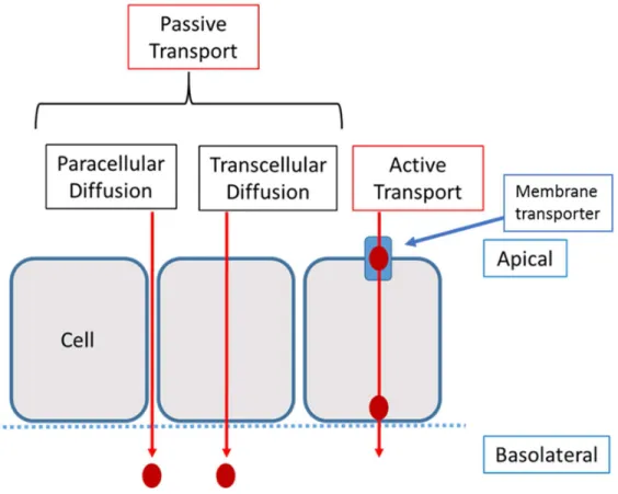
1.9 Permeability
Permeability is considered as a valuable parameter during the drug discovery process because it can significantly affect the ADME properties and it correlates to the velocity of a compound passage through a biological membrane barrier (Di & Kerns, 2016). Permeability extendedly affects the absorption and thus the bioavailability because a low permeable compound is not able to cross the cell membranes and ultimately interact with the biological target. Permeability also affects Distribution because it relates to the ability of the drugs to penetrate BBB and cell membranes. The ability or inability of a drug to permeate a biological membrane barrier (usually the intestinal membrane barrier) impacts on the drug’s efficacy. Therefore, a low permeability value results in a reduced bioavailability, which ultimately prevents the formulation