Comparing C4.5 and MST Classifier Using MapReduce
H. Anila Glory
1, R. Nithya
2, S. Irish Jeyapaul
31,2
Assistant Professor, Department of Computer Science and Engineering, Velammal Institute of Technology.
3
Assistant Professor, Department of Electronics and Communication Engineering, SCAD Engineering College.
---***---Abstract -
Now-a-days, with the aggregate of datagrowing at an unrivaled scale, extracting information from a big data and knowledge discovery has become a new challenge. Fuzzy Rough sets for knowledge acquisition have been successfully applied in data mining. There are many approaches to understand and manipulate data analysis. The most successful one is the Fuzzy Rough sets. Fuzzy Rough sets are a hybrid model obtained from the combination of Fuzzy set and rough set theory. It is a new mathematical tool for data analysis and handling imperfect data. For constructing a decision tree, here we used C4.5 and MST classifier. To identify the effective decision tree algorithm, Comparison is done between C4.5 and MST classifier. The recently introduced MapReduce technique has received much attention from both scientific community and industry for its applicability in big data analysis. MapReduce technique is employed to provide a fast and optimized way to classify large sets of real-life data by incorporating data pre-processing techniques using rough set induction in Hadoop framework in a parallel manner. Hadoop makes it doable to run applications on systems with thousands of nodes involving thousands of TB. Its DFS facilitates speedy knowledge transfer rates among nodes and permits the system to continue operational uninterrupted just in case of a node failure. This approach lowers the danger of harmful system failure, although a big variety of nodes become inoperative. To mine knowledge from big data and to find a effective decision tree algorithm, this paper is going to parallelize fuzzy rough set based methods for knowledge acquisition and decision tree construction for classification using MapReduce and implementing through Hadoop framework.
Key word:
Hadoop, MapReduce, Big Data, C4.5,
MST
1. INTRODUCTION
Data mining is the process of analysing data from different perspectives and summarizing it into useful information. The overall goal of the data mining process is to extract information from a data set and transform it into a knowledge base for further use. Nowadays, with the volume of data growing at an unprecedented rate, big data mining and knowledge discovery have become a new challenge. Big data is highly susceptible to noise, missing
values and inconsistency. Analyzing big data is quite time consuming process. The quality of the data affects the data mining results. In order to improve the quality of the data, data pre-processing step is essential. Data pre-processing is a data mining technique that involves transforming raw data into an understandable format. Real-world data is often incomplete, inconsistent, and lacking in certain behaviors, and is likely to contain many errors. Data pre-processing is a proven method of resolving such issues. Data pre-processing prepares raw data for further processing. Data pre-processing involves several methods. They are Data Cleaning, Data Integration, Data Transformation and Data Reduction. Data Cleaning means, Data that is to be analyze by data mining techniques can be incomplete (lacking attribute values), noisy(containing errors or outlier values), and inconsistent. Relevant data may not be recorded due to a misunderstanding, or because of equipment malfunctions. Data that were inconsistent with other recorded data may have been deleted. Data cleaning routines work to clean the data by filling in missing values, smoothing noisy data, identifying or removing outliers and resolving inconsistencies.
Data integration involves combining data residing in different sources and providing users with a unified view of these data. These sources include multiple databases, data cubes and flat files. This process becomes significant in a variety of situations, which include both commercial and scientific domains.
can help provide us with a better understanding of the data at large. The pre-processing steps described earlier must be applied to the data to help improve the accuracy, efficiency, and scalability of the classification process. This process is done by various methods like Decision tree Construction.
Decision tree induction is the learning of decision trees from class-labeled training tuples. A decision tree is a flowchart-like tree structure, where each internal node (non leaf node) denotes a test on an attribute, each branch represents an outcome of the test, and each leaf node (or terminal node) holds a class label. The topmost node in a tree is the root node.
Internal nodes are denoted by rectangles, and leaf nodes are denoted by ovals. Some decision tree algorithms produce only binary trees (where each internal node branches to exactly two other nodes), whereas others can produce non-binary trees. During tree construction, attribute selection measures are used to select the attribute that best partitions the tuples into distinct classes.
2. EXISTING SYSTEM
2.1 Neural Networks
Neural networks are widely used for classification of data by simulating the activity of the brain. In this method, the neural network is trained with various datasets with an attribute for each node such that it is processed to respond to a condition. Though this method produces good result, it is highly incomprehensive thus restricting its use.
2.2
CART
CART represents a major milestone in the evolution of Artificial Intelligence, Machine Learning and data mining. While CART citations can be found in almost any domain, far more appear in fields such as electrical engineering, biology, medical research and financial topics than, for example, in marketing research or sociology where other tree methods are more popular.
2.3
Decision Trees
Decision tree learning is a method commonly used in data mining for classification. Decision trees are popular
because they are practical and easy to understand. Rules can also be extracted from decision trees easily. Many algorithms, such as ID3 and C4.5 have been devised for decision tree construction. These algorithms are widely adopted and used in a wide range of applications such as image recognition, medical diagnosis, credit rating of loan applicants, scientific tests, fraud detection and target marketing.
2.4
ID3
ID3 algorithm uses entropy as the splitting criteria for the construction of decision trees. The entropy of a dataset can be considered to be how disordered it is. It has been shown that entropy is related to information, in the sense that the higher the entropy, or uncertainty, of some data, then the more information is required in order to completely describe that data. In building a decision tree, we aim to decrease the entropy of the dataset until we reach leaf nodes at which point the subset that we are left with is pure, or has zero entropy and represents instances all of one class. But entropy tends to favour the attribute which has a large number of values which is not suitable for all datasets.
2.5 C4.5
2.6
Rough Set
Rough set theory was developed by Zdzis law Pawlak in the early 1980's. It deals with the classificatory analysis of data tables. The data can be acquired from measurements or from human experts. The main goal of the rough set analysis is to synthesize approximation of concepts from the acquired data. A data set is represented as a table, where each row represents a case, an event, a patient, or simply an object. Every column represents an attribute (a variable, an observation, a property, etc.) that can be measured for each object; the attribute may be also supplied by a human expert or user. This table is called an information system. More formally, it is a pair A = (U;A), where U is a non-empty finite set of objects called the universe and A is a non-empty finite set of attributes[2]. A decision system (i.e. a decision table) expresses all the knowledge about the model. This table may be unnecessarily large in part because it is redundant in at least two ways. The same or indiscernible objects may be represented several times, or some of the attributes may be superfluous. We shall look into these issues now. The notion of equivalence is recalled first. A binary relation R X x X which is reflexive (i.e. an object is in relation with
itself xRx), symmetric (if xRy then yRx) and transitive (if xRy and yRz then xRz) is called an equivalence relation. The equivalence class of an element x 2 X consists of all objects y 2 X such that xRy.
Let A = (U;A) be an information system, then with any B A there is associated an equivalence relation
INDA(B)
INDA(B) ={(x; x`) U2 | B a(x) = a(x`)}
INDA(B) is called the B-indiscernibility relation. If (x, x`) ∈ INDA(B), then objects x and x` are indiscernible from each other by attributes from B. The equivalence classes of the Bin discernibility relation are denoted [x]B. The subscript A in the indiscernibility relation is usually omitted if it is clear which information system is meant.
An equivalence relation induces a partitioning of the universe .These partitions can be used to build new subsets of the universe. Subsets that are most often of interest have the same value of the outcome attribute. It
may happen, however, that a concept such as “Walk" cannot be defined in a crisp manner. For instance, two patients with the same symptoms may at times be differently diagnosed. In other words, it is not possible to induce a crisp (precise) description of such patients from the table. It is here that the notion of rough set emerges. Although we cannot define those patients crisply, it is possible to delineate the patients that certainly have a positive outcome, the patients that certainly do not have a positive outcome and, finally, the patients that belong to a boundary between the certain cases. If this boundary is non-empty, the set is rough. These notions are formally expressed as follows.
Let A = (U,A) be an information system and let B € A and X € U. We can approximate X using only the information contained in B by constructing the B-lower
and B-upper approximations of X, denoted BX and BX
respectively, where BX = {x | [x] B € X} and
BX = {x | [x] B X }.
The objects in BX can be with certainty classified as members of X on the basis of knowledge in B, while the objects in BX(Eq.1.2) can be only classified as possible members of X on the basis of knowledge in B. The set BNB(X) = BX BX is called the B-boundary region of X, and thus consists of those objects that we cannot decisively classify into X on the basis of knowledge in B. The set U BX is called the B-outside region of X and consists of those objects which can be with certainty classified as do not belonging to X (on the basis of knowledge in B). A set is said to be rough (respectively crisp) if the boundary region is non-empty (respectively empty).
If we are given a set of objects U called the
universe and an indiscernibility relation R U U,
representing our lack of knowledge about elements of U. Let X be a subset of U. We want to characterize the set X
with respect to R. To this end we will need the basic concepts of rough set theory given below.
The lower approximation of a set X with respect to R is the set of all objects, which can be for certain
The upperapproximation of a set X with respect to R is the set of all objects which can be possibly classified asX with respect to R (are possibly X in view of R).
The boundary region of a set X with respect to R is the set of all objects, which can be classified neither as Xnor as not-X with respect to R.
Set X is crisp (exact with respect to R), if the boundary region of X is empty.
Set X is rough (inexact with respect to R), if the boundary region of X is nonempty.Thus a set is rough (imprecise) if it has nonempty boundary region; otherwise the set is crisp (precise).
Rough set can be also characterized numerically by the following coefficient
called the accuracy of approximation, where |X| denotes the cardinality of X . Obviously
0 B(X) 1(Eq.1.3). If B(X) = 1, X is crisp with respect universe and hence the ability to perform classifications as the whole attribute set A does.
Another important issue in data analysis is discovering dependencies between attributes. Intuitively, a set of attributes D depends totally on a set of attributes C,, if all values of attributes from D are uniquely determined by values of attributes from C. Formally dependency can be defined in the following way. Let D and C be subsets of A. We will say that D depends on C in a degree k (0 < =k <=1), denoted C k D, I(C) I(D). That means that the partition generated by C is finer than the partition generated by D[1]. Notice, that the concept of
dependency discussed above corresponds to that considered in relational databases.
We often face a question whether we can remove some data from a data table preserving its basic properties, that is whether a table contains some superfluous data. In other words, we get the same accuracy of approximation and degree of dependencies as in the original table, however using smaller set of attributes.
As it follows from considerations concerning reduction of attributes, they cannot be equally important, and some of them can be eliminated from an information table without losing information contained in the table.
The idea of attribute reduction can be generalized by introducing a concept of significance of attributes, which enables us evaluation of attributes not only by two-valued scale, dispensable indispensable, but by assigning to an attribute a real number from the closed interval [0,1], expressing how important is an attribute in an information table.
Significance of an attribute can be evaluated by measuring effect of removing the attribute from an information table on classification defined by the table. Let us first start our consideration with decision tables.
Let C and D be sets of condition and decision attributes respectively and let a be a condition attribute,
i.e.,
a
C
. The number
(
C
,
D
)
expresses a degree of consistency of the decision table, or the degree of dependency between attributes C and D, or accuracy of approximation of U/D by C. We can ask how the coefficient)
,
(
C
D
changes when removing the attribute a, i.e., whatis the difference between
(
C
,
D
)
and
(
C
{
a
},
D
)
. Based on the difference value, decision is made as to whether the attribute is included in the set or not.3. PROPOSED SYSTEM
To provide a fast and optimized way to classify large sets of real-life data by incorporating data pre-processing techniques using rough set induction and employing MapReduce programming paradigm using Hadoop framework.
3.1 Missing Data Imputation
The input data set may have large number of missing values which may reduce the accuracy of data. Hot deck imputation is a method for handling missing data in which each missing value is replaced with an observed response from a similar unit. It is difficult to handle big data in hot deck imputation hence a equidistant hot deck imputation is proposed to fill in the missing values in parallel.
3.2 Fuzzy Rough Dimensionality Reduction
Dimensionality reduction is a process of selecting a map by which a sample in an m-dimensional measurement space is transformed into an object in a d -dimensional feature space, where d < m. The main objective of this task is to reduce dimensionality of the measurement space so that effective algorithms can be devised for effective classification. A dimensionality reduction algorithm is proposed based on fuzzy–rough sets, which simultaneously selects and extracts features from a given data set in parallel.
3.3 Parallel C4.5 Classifier
C4.5 builds decision trees from a set of training data in the same way as ID3, using the concept of information entropy. The training data is a
set of already classified samples. Each sample consists of a p-dimensional
entire decision tree is built. Maximum in gain ratio is computed as follows:
For an attribute A, relative to a collection of dataset D, the gain is:
Where ,
Where pi is the probability.
3.4 Parallel MST Classifier
The quality of the decision tree being built is determined by the criterion that is chosen for splitting. Xinmeng Zhang et.alhave proven that maximum similarity is a criterion that is effective in the quality of the decision tree. The total number of positive and negative outcomes for every attribute’s distinct attribute is computed in parallel using a MapReduce job. Using the data generated from the counter MapReduce job the similiarity of each attribute is computed. The attribute with the maximum similarity is chosen and added to the decision tree and subsets are generated with respect to each attribute value of the maximum similarity attribute and are marked as edges of the decision tree. The decision tree also called as MSTree is built using the outputs of the MapReduce jobs. Maximum similarity is computed as follows:
For an attribute A, the similarity Sim(A) is:
Where aiis the value of splitting attribute A and pi is the probability of splitting attribute.
Training set T is split into v subsets according to the value of splitting attribute A, T{T1,T2,...,Tv}, instances in Set T u
(1≤ u≤ v)that split by attribute value au belong to k classes
{c1,c2,...,ck}(1≤ k≤ m), the average similarity of Tu can be
computed by,
Where (1 ≤ j ≤ k), is the total similarity of all instances
belonging to same class cj , |T u| is the size of set T u .
The similarity of any two instances in subset Tu belonging
to same class is 1, and 0 otherwise.
4.
E
XPERIMENTAL RESULTSTwo classification algorithms, C4.5 and Maximum Similarity Tree based classification techniques were parallelized and implemented using MapReduce. The outcome of the roughset reduction was provided as input to both classification trees and error based pruning was carried out on the decision trees that are built by both classification algorithms. Confusion matrices were built for both decision trees and the confusion matrices are as follows:
In the confusion the (0,0)th entry represents positive outcome, (1,1) represents negative outcome, (0,1) false positive and (1,0) false negative. As both matrices suggest, the reach of MS Tree is greater than the reach of C4.5 based decision tree as the decision tree of MST algorithm was able to handle more number of records of the test data than the C4.5 based decision tree.
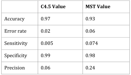
For classification the evaluation measures are given below:
C4.5 Value MST Value
Accuracy 0.97 0.93
Error rate 0.02 0.06
Sensitivity 0.005 0.074
Specificity 0.99 0.98
Precision 0.06 0.24
Chart 1: Evaluation graph for classifiers
As the graph suggests, even though MST was able to cover more number of records in the test data set, the number of false positives that it was generating is much higher than the C4.5 decision tree whose reach was lesser. Increasing the number of attributes used to build the decision tree improves the accuracy of the decision tree but increases the over fitting and the time taken to build the decision tree as well. Hence a fine balance is required to identify the number of attributes to be used. This is where the effectiveness of imputation and rough set reduction come into picture.
5. conclusion and future work
Data mining from big data has been a new challenge in recent years. Traditional rough sets based methods for knowledge discovery fail to deal with the growing data in applications. In this project, we have proposed parallel hot deck imputation for handling missing data and fuzzy rough set based methods for attribute selection using MapReduce. The experimental results show that parallel data pre-processing increases computational performance. The main work done in this project is the study of possibility of applying parallelism to the data reduction and classification process in data mining taking into account the recent Big Data computational problems in classification based on the various research perspectives. Decision tree construction are done in parallel using both C4.5 and MST classifier.
The experimental results show that parallel MST classifier gives better performance than C4.5 but, the error rate is high for MST classifier than C4.5. From the constructed Decision trees rules has been extracted for the purpose of Decision making. Our future work will focus on Decision tree pruning in parallel from the constructed decision tree to reduce the complexity.
R
EFERENCES[1]Pradipa Maji and Partha Garai, “Fuzzy-Rough Simultaneous Attribute Selection and Feature Extraction Algorithm”, IEEE Transactions on Cybernetics Vol 43, No 4, pp. 1166 – 1177,August 2013
[2] Turaj Amraee, Soheil Ranjbar, “Transient Instability Prediciton Using Decision Tree Technique”, IEEE Transactins on Power Systems, Vol 28, No 3, pg 3028 – 3037) August 2013
[3] Junbo Zhang, Tian Li, Yi Pan, “Parallel Rough Set Based Knowledge Acquisition Using MapReduce from Big Data”, BigMine ’12, Proceedings of the 1st International Workshop on Big Data, 2012
[4] Xiaojian, Yuchun, “Application of Decision Trees in Student Achievement Evaluation”, 2012 International Conference on Computer Science and Electronics Engineering, 2012
[5] Xiang Zhuoyuan, Zhang Lei, “Research on an Optimized C4.5 Algorithm Based on Rough Set Theory”, 2012 International Conference on Management of e-Commerce and e-Government , 2012
[6] Ashwinkumar U.M, Dr Anandakumar K.R, “Data Preparation by CFS and Essential approach for decision making using C4.5 for Medical data mining”, 2013 Third International Conference on Advanced Computing & Communication Technologies, 2013
[7] Sridevi T, Murugesan A, “Rough set theory based attribute reduction for breast cancer diagnosis”, Indian J. Innovations Dev, Vol 1, No 5, pg 309 – 313, May 2012
BIOGRAPHIES
H.ANILA GLORY, Assistant Professor, Department of Computer Science and engineering, Velammal Institute of Technology, Chennai, India. E-mail: [email protected]
R. NITHYA, Assistant Professor, Department of Computer Science and engineering, Velammal Institute of Technology,Chennai,
India. E-mail: