Autonomous Navigation Algorithms for Mobile Robots based on LiDAR technogies

(1)

UNIVERSIDAD POLITÉCNICA DE

CARTAGENA

Escuela Técnica Superior de Ingeniería Industrial

Autonomous Navigation Algorithms

for Mobile Robots based on LiDAR

Technologies

TRABAJO FIN DE GRADO

GRADO EN INGENIERÍA DE TECNOLOGÍAS INDUSTRIALES

Autor: Leanne Rebecca Miller

Director: Pedro Javier Navarro Lorente

Codirector: Carlos Fernández Andrés

(2)

(3)

Abstract

In recent years, the use of mobile robots for performing different tasks is increasing rapidly. It is now common to find robotic systems in industrial environments, military applications, agricul-tural systems and even in businesses carrying out increasingly sophisticated tasks. The develop-ment in the mobile robotics field has moved on from research in universities and businesses to use in everyday environments. The advances made in mobile robotics have been transferred to other fields, such as autonomous driving or space exploration. The obstacle avoidance algo-rithms, local and global path planning techniques and perception systems developed in mobile robotics are used for the new self-driving vehicles.

This dissertation presents a navigation system for a mobile robot with a differential steering system, which combines different path planning and obstacle avoidance algorithms. The algo-rithms implemented are combined with a localization system using different sensors installed on the robot (encoders, LiDAR, IMUs, etc). The main algorithms used in this project are: The A* algorithm, the Vector Field Histogram and dead reckoning.

Resumen

En los últimos años, el uso de los robots móviles para realizar diferentes tareas ha crecido de forma exponencial. Es habitual encontrar sistemas robotizados en ambientes industriales, aplicaciones militares, sistemas agrícolas e incluso en empresas realizado tareas cada vez más sofisticadas. Los desarrollos en robótica móvil han pasado del campo de la investigación en Universidades y empresas al entorno cotidiano. Los avances en robótica móvil han sido transferidos a otros campos como la conducción autónoma o la exploración espacial. Los algoritmos de evitación de obstáculos, los planificadores locales y globales de trayectorias y los sistemas de percepción desarrollados en la robótica móvil, son utilizados en los nuevos vehículos sin conductor.

Este trabajo final de grado presenta un sistema de navegación para un robot móvil de tipo diferencial, que combina distintos algoritmos de creación de trayectorias y evitación de obstáculos. Los algoritmos implementados se combinan con un sistema de localización utilizando diferentes sensores instalados en el robot (encoders, LiDAR, IMUs, etc.). Los principales algoritmos usados son: El algoritmo A*, el Vector Field Histogram y la navegación por estimación (dead reckoning).

(4)

(5)

List of Figures

Figure 1.1 Google's self-driving car with LiDAR sensor ... 10

Figure 2.1 Fetch Robotics’ Freight 500 Robot ... 14

Figure 2.2 RoboCourier transporting robot ... 15

Figure 2.3. iRobot Roomba vacuum robot (Left), Desktop Robot cleaner (Right) ... 15

Figure 2.4 TALON Tracked Military Robot, USA ... 16

Figure 2.5 DOGO Tactical combat robot ... 17

Figure 2.6. Pioneer P3-DX... 17

Figure 2.7 TurtleBot ... 18

Figure 2.8 Ultrasonic sensor range (Siegwart) ... 20

Figure 2.9 Velodyne VLP-16 (Left) and Velodyne HDL-64E (Right) ... 21

Figure 2.10 Calculating position with an IMU (Siegwart) ... 21

Figure 2.11 Differential Drive Robot ... 23

Figure 2.12 Instantaneous Centre of Curvature ... 24

Figure 3.1 Exact cell decomposition ... 26

Figure 3.2 Effect of grid resolution for approximate cell decomposition ... 27

Figure 3.3 Adaptive cell decomposition ... 28

Figure 3.4 Voronoi diagram ... 28

Figure 3.5 Robot world divided into a grid ... 29

Figure 3.6 f(n), g(n) and h(n) scores for the previous configuration ... 30

Figure 3.7 A* Algorithm after two iterations ... 30

Figure 3.8 Final Path ... 31

Figure 3.9 Potential field generated by an obstacle (repulsive) and a goal (attractive) ... 32

Figure 3.10 Path created by potential field forces ... 32

Figure 3.11 U-Shaped obstacle that causes a local minimum ... 33

Figure 3.12 Comparison between Bug1 and Bug2 algorithms ... 33

Figure 3.13 Polar Histogram ... 34

Figure 4.1 LabVIEW VI. Front panel (left), Block diagram (right) ... 36

Figure 4.2 LabVIEW Robotics Simulator ... 37

Figure 4.3 National Instruments DaNI Robot ... 37

Figure 4.4 Hokuyo Laser Scanner ... 38

Figure 4.5 6DOF IMU ... 38

Figure 4.6 HMC6343 Compass Module ... 38

Figure 4.7 Robot Scene Environment ... 39

Figure 4.8 Customized Robot Environment ... 39

Figure 4.9 Simulator Initialization ... 40

Figure 4.10 Robot scene rotated with origin in top left corner ... 41

Figure 4.11 Second robot environment rotated with origin in top left corner ... 42

Figure 4.12 A* Algorithm in LabVIEW ... 43

Figure 4.13 Steering frame for DaNI robot ... 43

Figure 4.14 Simulated robot real position and heading ... 44

Figure 4.15 Advanced VFH VI ... 45

Figure 4.16 User Interface ... 47

Figure 5.1 Robot environment for first test ... 50

(8)

Figure 5.3 Path chosen by the robot in the first simulation ... 51

Figure 5.4 Obstacle avoidance ... 52

Figure 5.5 Robot re-joins the planned path once past the obstacle ... 52

Figure 5.6 Final Positions of DaNI after the first simulation ... 53

Figure 5.7 Path chosen for the second set of tests ... 54

Figure 5.8 User Interface with estimated position ... 54

Figure 5.9 The robot leaves the path enough to avoid the obstacle ... 55

Figure 5.10 Final position obtained in test with dead reckoning ... 55

Figure 5.11 GUI for the second test ... 56

Figure 5.12 Modification of the pose calculations ... 57

Figure 5.13 Final position after improving dead reckoning ... 57

Figure 5.14 Final position after corrections ... 58

Figure 5.15 Third test simulation ... 59

Figure 5.16 Simulation at 0.35m/s ... 59

Figure 5.17 Final Positions of DaNI at 0.30m/s ... 61

Figure 5.18 Final positions after changing the maximum speed ... 62

Figure 5.19 Average final positions of the robot... 63

Figure 5.20 Trajectory tracking control ... 64

Figure 5.21 ANN Software user interface ... 64

Figure 5.22 ANN Training ... 65

Figure 5.23 Trajectory planning subVI ... 65

Figure 5.24 Virtual Vehicle Posture subVI ... 66

Figure 5.25 ANN Get Posture subVI ... 66

Figure 5.26 ANN Tracking wheel controller subVI ... 66

Figure 5.27 Robot scene modified for ANN comparison ... 67

Figure 5.28 Trajectory planned by A-Star algorithm ... 67

Figure 5.29 User interface used for the comparison ... 68

Figure 5.30 ANN Trajectory and user interface... 68

Figure 5.31 Final Positions of DaNI in the third simulation ... 70

Figure 6.1 Example of a 2D occupancy map for a vehicle (P.J. Navarro, 2017) ... 73

(9)

CHAPTER 1

(10)

10

1.1 Motivation

In recent years, the number of automobile companies and universities researching into autonomous vehicles has increased rapidly. In order to completely achieve autonomous driving, various sub-systems have to be combined, such as perception systems, a localization system and navigation and trajectory planning systems. It is very important that an autonomous vehicle or robot knows where it is situated so it can carry out path planning more effectively with less error. In addition to the algorithms used, the accuracy of localization depends on the precision of the sensors used.

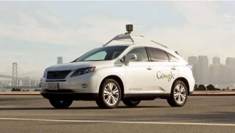
The motivation of this project is to acquire knowledge in the field of autonomous navigation systems and the algorithms and localization methods used in mobile robotics. In order to achieve this, problems of increasing difficulty related to mobile robots will be solved. These missions will be carried out in different environments designed on a simulator where a mobile robot will have to avoid obstacles, create trajectories, calculate its position and reach a target. In the future, the software developed could be adapted for use on an autonomous vehicle (Figure 1.1).

Figure 1.1 Google's self-driving car with LiDAR sensor

Autonomous vehicles and mobile robots can either be controlled by teleoperation or they can be programmed to perform operations autonomously. In this project, a navigation system has been designed for a small mobile robot so that it can operate autonomously in an environment, without the need for human intervention. The system involves driving from an initial position to a goal whilst avoiding obstacles and choosing the best trajectory.

The mobile robot navigation problem was defined in 1991 by Leonard and Durrant-Whyte [1] and consists in solving the following three questions: “Where am I?”, “Where am I going?” and “How do I get there?” from the robot’s point of view. The first question requires the mobile robot localization problem to be solved, while the second and third in addition are related to path planning and motion.

To solve the localization problem adequately, information from different sensors, such as encoders and inertial sensors, must be combined in what is known as sensor fusion. This information alone is not enough and to achieve accurate results must be analysed and corrected using a filter. The most common filter is called the Kalman filter which used a statistical approach.

The path planning and motion problem involves creating a trajectory from the starting position of the robot to a goal. This is known as global navigation and this must be combined with local navigation to be more effective. Local navigation is the avoidance of obstacles that were

(11)

Chapter 1. Introduction

11 unknown when programming the original path. If unexpected obstacles appear in the way of the robot, the robot must avoid them and still head towards the final goal.

1.2 Objectives of the Project

The main objective of this project is the study and development of navigation, localization and obstacle avoidance algorithms for a mobile robot. To detect the environment and obstacles, a LiDAR (Light Detection and Ranging) sensor will be used as the main perception system. Other sensors that will be used include the robot encoders and an inertial measurement unit.

The project has been divided into six goals which are the following:

- Analysis of the state of the art in mobile robotics and navigation. Research about the current path planning and goal seeking algorithms and perception methods.

- Develop a navigation application including a user interface and obstacle avoidance algorithms that allow a robot to drive autonomously to a position defined by the user. - Program a localization system using inertial sensors and encoders. In order to

successfully carry out the path planning algorithms, it is important that the robot has a good localization system and knows where it is situated. The data obtained from the different sensors should be combined using a suitable method.

- Carry out tests using a mobile robotics simulator. Create an appropriate simulated environment with realistic features such as walls and doors.

- Perform tests and compare the results obtained with the mobile robot to those obtained with the robotics simulator. Check that the objectives have been met analyse the final results.

1.3 Structure of the Project

Chapter 1. Introduction.

In this chapter, the motivation for carrying out this project will be defined, along with the objectives of the project.

Chapter 2. State of the Art in Mobile Robotics.

A study of the current state of the art of the mobile robot industry will be carried out. The autonomous mobile robot navigation problem will be explained. The different subsystems that make up an autonomous navigation system will be studied: Perception, navigation and kinematics of a differential drive robot will be discussed.

Chapter 3. Navigation Algorithms.

The most common and well known global and local navigation algorithms currently used for autonomous mobile robots will be explained in detail.

(12)

12

Chapter 4. Implementation using a Robotics Simulator.

In this chapter, the software, the different simulated environments designed and the sensors used will be described. The functions and algorithms used to develop the software will be explained.

Chapter 5. Simulated Tests and Results.

The tests carried out with the robotics simulator will be described and the results obtained in different conditions and at different speeds will be compared. The software will also be compared to an existing navigation program.

Chapter 6. Conclusions and Future Projects.

The conclusions drawn from the project and the original objectives will be discussed. Future projects will be proposed.

(13)

CHAPTER 2

(14)

14

2.1 Mobile Robotics Industry

Since robots were introduced in factories in the early 1960s, they have evolved rapidly and are now capable of performing complicated and tedious tasks along the assembly line with a very high precision. However, this type of manipulator robots has one important disadvantage which is the lack of mobility. Unlike fixed base industrial robot arms, mobile robots can operate in large areas and explore environments that could be potentially dangerous to humans.

Mobile robots usually move by means of a set of wheels or articulated legs. Legged robots require greater mechanical complexity due to the fact higher degrees of freedom are needed compared to wheeled robots. In addition, on flat ground wheeled robots are generally more stable since all wheels are designed to be in contact with the ground [2].

Existing mobile robots can be separated into three main groups: Commercial robots, military robots and robots designed for research.

2.1.1 Autonomous Commercial Robots

Apart from working in hostile environments, it is also becoming more common to see robots working alongside humans, performing heavy and tedious tasks. On factory floors, Automated Guided Vehicles (AGVs) are being replaced by Autonomous Mobile Robots [3], with the latter capable of avoiding obstacles and redirecting their paths if necessary, unlike the AGVs which are stuck on a predetermined track.

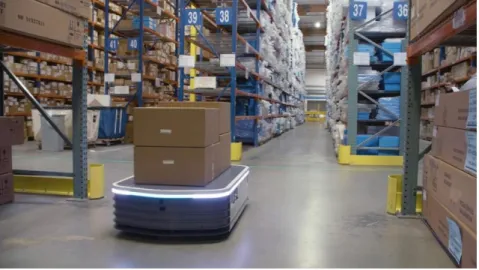
An example of this type of commercial robot are Fetch Robotics’ autonomous freight robots (Figure 2.1) which are designed to replace forklifts and trolleys in warehouses and can transport up to 1500kg of payload. These transporting robots navigate around the warehouses using LiDAR sensors and a RGB camera on the front [4].

Figure 2.1 Fetch Robotics’ Freight 500 Robot

Another example of an autonomous robot that works alongside humans is the RoboCourier from Swisslog (Figure 2.2). This robot is used for light weight hospital material transport and has automatic interfaces for doors and lifts and allows the safe transport of laboratory specimens and supplies [5]. The robot uses LiDAR laser sensors for navigation and navigates autonomously through busy hallways avoiding obstacles.

(15)

Chapter 2. State of the Art in Mobile Robotics

15 Figure 2.2 RoboCourier transporting robot

In recent years, a large variety of domestic robots have also become available to consumers, one of the most common is the autonomous vacuum cleaner. These robots vary greatly in cleaning capacity and price, with some having over five different cleaning modes. Some of the more complex vacuum robots can be programmed to clean in function of the size of the room or the amount or type of dirt to be cleaned and are even capable of mapping their environment and the surface area to be covered.

The iRobot Roomba (Figure 2.3 (Left)) is one of the most advanced models of vacuum robot and uses Simultaneous Localization and Mapping (SLAM) so it knows where it has already been and which areas still need to be cleaned [6]. These robots use infrared sensors to detect the surface underneath them to avoid falling off stairs, and have bumpers to detect obstacles. Infrared sensors are also used for close wall following, this way the robot reduces the amount of times it bumps into furniture, etc. There are many varieties of cleaning robot, including smaller desktop robots (Figure 2.3 (Right)).

(16)

16

2.1.2 Military Mobile Robots

As robots are becoming more sophisticated and reliable, they are increasingly being used for military applications. Robots are starting to play an important role in patrolling and can perform dangerous missions and deal with explosives [7]. Military robots are different to industrial mobile robots as they are normally teleoperated and do not often carry out missions autonomously. This is usually for safety reasons and the robots are under the complete control of the operator.

Mobile military robots must also be able to operate on many types of terrain, which in many cases can be harsh and dangerous, and this will mean more restrictions when designing the robot. Data security is another vital requirement for military operations. The wireless data transmission between the robot and operator must be secured both ways so that there can be no interference with the data and images sent to and from the robot.

One of the most widely used military robots in the USA is TALON [8]. TALON is an unmanned, tracked military robot developed in the United States, designed to protect soldiers against explosive threats (Figure 2.4). The robot can transport heavy loads, perform explosive disposal missions, mine detection and rescue missions. TALON can be operated from up to one kilometre away and can work in contaminated areas for extended periods of time. The robot features a manipulator arm which can rotate 360˚ and has a microphone and loudspeaker. The robot can be equipped with a diverse range of sensors for gas, radiation and chemical detection as well as an extra rotating shoulder for heavy lifting. Additional firing circuits and a range of weapons such as shotguns can be installed.

Figure 2.4 TALON Tracked Military Robot, USA

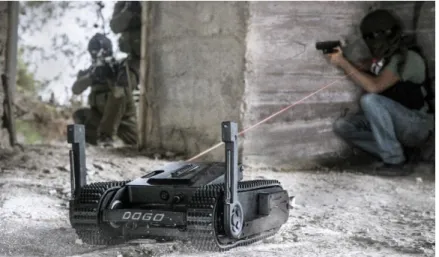
Another important military robot is General Robotics’ DOGO [9]. The DOGO is a tactical combat robot armed with a 9mm pistol and provides live video footage using an omnidirectional vision system with eight video cameras (Figure 2.5). The robot has an interface which allows the operator to aim the weapon by simply touching the target on the screen. DOGO can operate on rough terrain and climb stairs, making it suitable for urban and rural warfare.

(17)

17 Figure 2.5 DOGO Tactical combat robot

2.1.3 Mobile Robots used for Research

Mobile robots have a broad range of applications, but to achieve the successful design of a mobile robot, many different areas of knowledge must be combined. To solve the localization and navigation problems a good understanding of electronics, sensors, programming and computer algorithms is necessary. For the locomotion, it is also important to have knowledge of kinematics, dynamics and mechanics.

Research on localization and navigation tasks for robots can be carried out using standard robot platforms designed for use in laboratory environments. These robots usually come with a few basic sensors such as ultrasonic sensors and wheel encoders and can be customized by adding LiDAR sensors, cameras or other mechanisms.

Figure 2.6. Pioneer P3-DX

One of the most popular research robots is the Pioneer P3-DX (Figure 2.6). Pioneer P3-DX is a differential drive robot with 16 ultrasonic sensors and an embedded motion controller. Many different sensors and actuators can be added, making this robot very versatile.

(18)

18

Figure 2.7 TurtleBot

TurtleBot is an open source robot designed for use in research and education [10]. With its basic components, users can carry out Simultaneous Localization and Mapping (SLAM) and follow a person’s legs as they walk. TurtleBot uses the open source Robot Operating System platform and different sensors and actuators can be added to the basic platform which consists of a Kinect sensor (Figure 2.7).

2.2 Robotic Subsystems

Autonomous mobile robots combine different subsystems to perform the actions defined by the operator. Each subsystem has a certain task to carry out and the way these subsystems interact with each other defines the behaviour of an autonomous robot.

According to Siegwart [2], in order to accomplish autonomous navigation, four subsystems need to be successfully implemented:

- Perception: Consists in the robot extracting meaningful data about its environment

from the sensors. Usually the information acquired from more than one type of sensor is used to reduce error, the readings from the different sensors can be combined using sensor fusion algorithms.

- Localization: The robot must know its relative position in the environment. This is one

of the hardest parts of robot navigation due to sensor inaccuracies. The localization problem involves more than just determining the absolute and relative pose of the robot, map building and landmark extraction are also important components of this subsystem.

- Cognition: Also known as path planning, the robot must decide how to reach its goal,

choosing a suitable trajectory and avoiding obstacles.

- Motion Control: The path calculated previously must be converted into velocities or the

required motor input, so that the robot can carry out the planned action and reach the desired goal.

(19)

19

2.3 Perception and Localization

Perception is the ability of the robot to detect the environment that it is in and the obstacles in its path. The precision of the robot localization problem depends on the capacity of the sensors available on the robot and the accuracy of the algorithms used to process the raw data. The different sensors that can be used to obtain the posture of the robot are: wheel encoders, LiDAR and time of flight (TOF) sensors such as 2D and 3D laser scanners and ultrasonic sensors, inertial measurement sensors, artificial vision (TOF and artificial vision cameras), and GPS.

However, to obtain a precise information about the robot’s environment it is necessary to combine these perception methods. Although GPS systems are good for outdoor robots, it is still necessary to have an alternative localization method, as GPS is no good in tunnels or indoor environments such as underground carparks. It is also necessary to combine artificial vision systems with other methods of positioning as cameras can be very sensitive to different light levels, and are especially sensitive to direct sunlight.

Robot localization is the ability of the robot to determine its position in the environment and is part of the perception problem. The position of the robot is very important as to carry out the assigned tasks correctly, the robot must know exactly where it is. The robot relies on the information obtained from the sensors to calculate its position, in outdoor environments, GPS is normally used, meanwhile for indoor situations other types of sensors must be available. The accuracy of localization does not only depend on the algorithms used, but also on the types of sensors and their precision, the type of surface that the robot is on, and the type of objects, as the sensor readings can vary depending on the material of the objects.

The sensors used on mobile robots can be classified into two groups:

1. Proprioceptive sensors, which measure the internal magnitudes of the robot, such as the motor speed or battery voltage.

2. Exteroceptive sensors, which acquire information about the robot’s surroundings, such as the distance to obstacles.

2.3.1 Odometry

Encoders are proprioceptive sensors that measure the wheel rotation while the robot is moving. Optical encoders are the most commonly used type of odometry sensor and use a photodetector to sense the reflection or interruption of a beam of light on a spinning disk attached to a motor. With the physical dimensions of the robot, it is possible to calculate the forward and angular velocities of the robot from the angular velocities of each wheel. The distance travelled by the robot, and therefore its position can be obtained by integrating the forward and angular velocities calculated previously.

2.3.2 Ranging Sensors

Ranging sensors are used to measure the proximity of features in the environment to the robot without physical contact with the objects. A signal (sound or light) is emitted by the sensor and the time taken for signal to be reflected back to the sensor is converted into a distance. This is known as time-of-flight ranging. The accuracy of the time-of-flight sensors depends mainly on

(20)

20

the speed of the robot, the material of the objects in the environment, the variation in the propagation speed and inaccuracies in the arrival time of the return signal.

Early localization systems used sonar sensors, however 2D and 3D laser scanners are now more commonly used as they are faster and more reliable. For indoor localization, 2D scanners are normally used, due to the fact that 3D scanners are larger and more difficult to install on smaller indoor robots.

2.3.2.1 Ultrasonic Sensors

Ultrasonic sensors calculate the distance to objects by emitting a sound wave at a specific frequency and measuring the time it takes for the wave to bounce back. Ultrasonic sensors are one of the most affordable ranging sensors and were widely used before the 2D laser scanner became available [11], however they have some important drawbacks. Sound propagates in a cone-like manner, with an opening angle of between 20 and 40 degrees (Figure 2.8), which means that instead of getting precise directional information, the sensor only tells us that there is an object in this area.

Figure 2.8 Ultrasonic sensor range (Siegwart)

Another important disadvantage of ultrasonic sensors is they can give bad readings with some materials if the sound wave is absorbed instead of reflected. The waves can also be reflected wide of the receiver leaving the object undetected.

2.3.2.2 Laser Scanners (LiDAR)

Laser scanners have significant improvements compared to ultrasonic sensors. These sensors emit beams of laser light instead of sound. In addition to giving very precise distance measurements, the directional information acquired is also much more reliable.

On mobile robots, the most common LiDAR sensors are 2D laser scanners, because 3D laser scanners are usually too large and heavy. The biggest problem with 2D scanners is that they only detect the environment on a flat plane at the level of the sensor, so for some applications this is not sufficient. However, there are some smaller models of 3D LiDAR scanners such as the Velodyne VLP-16 (Figure 2.9) which are suitable for smaller mobile robots and provide a complete view of the environment where the robot is operating.

(21)

21 Figure 2.9 Velodyne VLP-16 (Left) and Velodyne HDL-64E (Right)

2.3.3 Inertial Navigation System

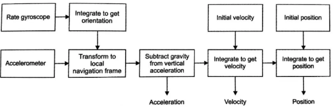
Inertial Navigation Systems use accelerometers, gyroscopes and compasses to estimate the position of the robot (Figure 2.10). Inertial Measurement Units (IMU) are often used for navigation on ships and aircraft as well as in robotics.

IMUs usually consist of a 3-axis accelerometer and a 3-axis gyroscope, although it is becoming increasingly common to include a heading sensor such as a compass and even thermometers and barometers.

Accelerometers measure the external forces acting upon them. These forces can be static such as gravity or dynamic. The static acceleration can be used to find out the angle the device is tilted at with respect to the Earth. The dynamic acceleration can be used to analyse the movement and calculate position.

Gyroscopes are devices that measure rotational motion. The angular velocity can be integrated to obtain the orientation. These sensors are often used on balancing robots to keep them upright.

Figure 2.10 Calculating position with an IMU (Siegwart)

Compasses, unlike accelerometer and gyroscopes, are exteroceptive sensors and measure the magnetic field which is used for calculating the heading. The disadvantage of compasses is that they are easily affected by exterior magnetic fields which corrupts the data supplied by these sensors.

(22)

22

2.4 Path Planning

In order to operate autonomously, robots must be capable of finding their way from an initial position to a goal defined by the user. To operate autonomously, the robot must compute the most effective trajectory in a known environment whilst avoiding obstacles. In addition to creating a path around known obstacles, if there are any unexpected obstructions along the path, the robot must compute a new path so it can reach the final goal.

The path planning problem can be divided into two distinct parts:

- Global navigation: Involves planning a trajectory from the robot’s current position to a

goal. To do this, the robot needs a map, either complete or partial, especially in an environment that contains walls and corridors.

- Local navigation: Although the robot will usually have a map, this can be incomplete

and there can be unpredicted obstacles in the robot’s path. To reach the goal, the robot must avoid the obstacles in the most efficient manner possible and try to head as much towards the goal as possible.

To improve the performance of the robot, both techniques should be combined, allowing the robot to avoid unexpected obstacles whilst still heading towards the final goal. If only local navigation is used, although the robot will avoid obstacles and still head towards the goal, it will spend more time trying to find a clear path and could get lost. Global navigation is not sufficient alone either, as if there are any moving obstacles or the map given to the robot is incomplete, it will not be able to situate itself as precisely and could collide with the unknown obstacles. The path planning algorithms most commonly used will be explained in detail in the following chapter.

2.5 Motion Control: Kinematics for a Differential Drive Robot

Before navigation and path planning can be carried out, it is important to understand the mechanical behaviour of the robot. This is known as kinematics and involves the study of the motion without considering the forces involved.

For a robot operating on a horizontal plane, there are three variables that define the pose of the robot: The x and y coordinates of the position on the plane and the heading which is the orientation with respect to the vertical axis. The possible movements that the robot can perform depend on the type and distribution of its wheels. A differential robot has two separately controlled motors which move wheels independently on the same axis on either side of the robot (Figure 2.11). If the forward velocity Ẋ, the lateral velocity Ẏ and the angular velocity ω are known, with the dimensions of the robot, the velocities vL and vR of each wheel can be

calculated.

Differential drive robots are very sensitive to slight changes in the velocity of the wheels and a small error in the relative velocity between the wheels can cause great error in the trajectory.

(23)

23 Figure 2.11 Differential Drive Robot

For this type of robot there are three simple types of motion:

1. If vL = vR the robot will move forwards or backwards in a straight line, the angular velocity

is 0 and there is no rotation.

2. If vL = -vR then the robot will turn in place around the midpoint of the wheel axis. The

forward velocity is zero.

3. If vR = 0, the robot will turn in a circle around the right wheel. If vL = 0, the rotation will

be around the left wheel.

When one wheel rotates at a higher speed than the other, the robot will turn around a point which lies either to the right or the left along the wheel axis. This point is known as the Instantaneous Centre of Curvature (ICC) and is the centre of the circular path described by the robot.

For differential drive robot, there are two geometrical parameters that define the motion of the robot: The wheel radius and the length of the wheel axis. For these robots, there is no lateral velocity and the velocities for each individual wheel can be calculated from the rate of rotation around the ICC:

𝑉𝑟 = 𝜔 (𝑅 + 𝐿 2) 𝑉𝑙 = 𝜔 (𝑅 − 𝐿 2)

With R being the radius from the ICC to the midpoint of the wheel axis, L the distance between the two wheels and ω the angular velocity (Figure 2.12).

The distance travelled by a robot can be calculated with the radius of the wheel and the angle the wheel has rotated. If the robot is travelling forward, the distance s travelled with one complete turn of the wheel is:

𝑠 = 2𝜋𝑟

(24)

24

Figure 2.12 Instantaneous Centre of Curvature Therefore, the distance travelled can be generally expressed as:

𝑠 = 𝛼𝑟

Where α is the angle rotated (in radians). The angle rotated or the angular velocity of the wheels of the robot is obtained from the encoders. The encoders can be used to obtain an estimation of the pose of the robot. With the velocities of each wheel, the overall angular velocity and forward velocity can be calculated. If these are then integrated, and added to the previous x, y and θ vales the current position is obtained. However, it is important to take into account that encoders alone are not sufficient for calculating the pose of the robot as they accumulate a lot of error.

(25)

CHAPTER 3

(26)

26

3.1 Environment Mapping Techniques

Before graph based searches can be performed, the environment must be divided into free and occupied space and represented on a graph. When choosing which mapping technique to use, three key factors must be considered:

- The precision with which the robot should reach its target. - The types of features that need to be represented on the graph.

- The computational cost of the map, as this depends on the complexity of the graph. Robot mapping methods can be continuous or discrete. Continuous mapping consists of creating a map with the data from the sensors on board the robot. As only the sensor readings are used, these maps are usually very precise. However, if there are many features the computation cost will be high and to store the map a lot of memory will be needed.

Discrete mapping techniques basically decompose the environment, distinguishing the features from open space. These types of maps are transformed into graphs with a much lower computational cost, making path planning easier to compute. The disadvantage is the precision, as the features are usually represented approximately. In this project, discrete mapping methods will be used.

3.1.1 Exact Cell Decomposition

One common technique is cell decomposition, which can either be exact or approximate. In exact cell decomposition, the cells can only be completely occupied or completely free (Figure 3.1). The position of the robot inside each cell is not important, but the robot must be able to move from its current cell to the adjacent cells. The disadvantage of this method is that the exact path of the robot is not defined, therefore the exact position of the robot in the cell is unknown.

(27)

Chapter 3. Navigation Algorithms

27

3.1.2 Approximate Cell Decomposition

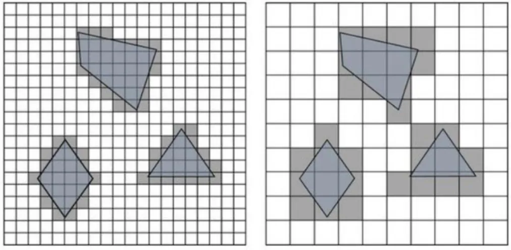
Approximate cell decomposition is one of the most popular techniques due to the simplicity of grid representations. The most common method is the occupancy grid. The robot environment is divided into a grid with fixed sized squares, therefore obstacles are represented approximately. A drawback of this method is that a cell is classed as an obstacle even though it may not be completely occupied, and depending on the size of the grid squares, narrow passages can be lost [12].

It is also important when choosing the size of the grid squares to consider the size of the robot, as if the robot is bigger than the cell size, it is not possible to locate the robot in just one position. This reduces the accuracy of the grid when defining obstacles and for large robots this technique would not be suitable.

Figure 3.2 Effect of grid resolution for approximate cell decomposition

The size of the features in the environment must also be considered, as if there are small features, the resolution of the grid must be higher, but if the obstacles are large, then only a low resolution is needed. The resolution used also depends on the accuracy and time available for reaching the goal. If the robot needs to arrive quickly to the goal, a higher resolution can be used allowing the robot to pass through smaller gaps that would be classed as obstacles with a lower resolution (Figure 3.2).

3.1.3 Adaptive Cell Decomposition

This method is analogous to the approximate cell decomposition, as it also divides the environment into a grid. However, with this technique, the size of the squares depends on their proximity to an obstacle (Figure 3.3).

This method divides the environment into two squares, then uses a recursive decomposition procedure for each square. Each cell should either be free space or an obstacle, if both values are present in a cell, this cell is divided into four equal sized cells. This procedure is then applied to each of the new cells. Once a cell contains only free space or an obstacle, it remains the same size. This iterative process is carried out until the whole environment consists of cells of either obstacle or free space.

(28)

28

Figure 3.3 Adaptive cell decomposition

The precision of this method depends on the minimum cell size defined and the allowed computational cost.

3.1.4 Voronoi Diagram

A different approach for creating a map is the Voronoi diagram. This is a road map method that tries to maximize the distance between the robot and the obstacles [2]. This technique calculates divides the environment into Voronoi cells, with each one containing an obstacle or point. The cell boundaries are calculated as the midpoints between the obstacles. These points are joined together forming paths (Figure 3.4).

Figure 3.4 Voronoi diagram

The advantage of this method is that the robot will always be as far away as possible from the obstacles. Also, this type of diagram is very easy for the robot to follow using simple control rules. The disadvantage is that the computational cost is higher than for other methods because of the cost of calculating the equidistant points.

3.2 Path Planning Algorithms

The path planning problem, according to Dudek [13], consists in creating a path in an environment between the initial pose of the robot and the goal position in a such a way that the trajectory and planned motion is consistent with the kinematic constraints of the robot whist also avoiding collision. Path planning is the decision-making part of navigation, as it is responsible for finding the quickest and safest way to reach the goal.

(29)

29 Before carrying out any type of path planning, the robot environment must be transformed into a suitable discrete map. There are two general strategies according to Siegwart [2]:

- Graph search: First a graph of the robot world is built, then it is searched to find the best

path.

- Potential field planning: Consists in imposing a mathematical function directly onto the

space. The gradient of this function is then followed to the goal.

**3.2.1 A* Path Planning Algorithm**

The A* algorithm [14] is a graph search technique that finds the optimal path with the lowest cost from an initial node to any position in a previously defined graph. This method is similar to Dijkstra’s algorithm [15], but includes a heuristic function to try and reduce the number of nodes explored.

Before the algorithm can be carried out, the robot world must be divided into a grid, which can be defined as a two-dimensional array. Every grid square must be classified as either a free space or an obstacle (Figure 3.5). All of the squares (also referred to as cells or nodes) originally have their status set as unvisited or obstacle. The shortest path is created by evaluating the adjacent cells and calculating a cost function to choose the best next move.

Figure 3.5 Robot world divided into a grid The cost function f(n) is defined as:

𝑓(𝑛) = 𝑔(𝑛) + ℎ(𝑛)

The function g(n) is the cost to move from the starting cell to any other position in the grid. The cost to move horizontally or vertically is given a value, and the cost to move diagonally is the square root of 2 times the cost of moving horizontally or vertically.

The function h(n) is the heuristic function which gives additional knowledge about the graph, making the algorithm more efficient. The heuristic is the estimated cost to move from the current position to the goal node. The performance of the algorithm depends on the heuristic used, but the efficiency on average is much better than that of the Dijkstra algorithm.

If the heuristic function h(n) is 0, the A* algorithm will behave the same as Dijkstra’s and will be slower. If h(n) has a very high value, the algorithm will run very quickly, however the path may not be the shortest possible route. Some heuristics commonly used are the Manhattan distance (distance to target only moving horizontally and vertically), diagonal distance and the Euclidian

(30)

30

distance. The heuristic used in this project is calculated estimating the Euclidian distance to target cell. This method estimates the absolute distance to the goal, ignoring any obstacles that might be in the way.

In the first step of the algorithm, all of the cells that are adjacent to the first cell are either added to an open list or a closed list. The open list contains all of the cells that are possible candidates for the next move. The closed list contains all of the cells that have already been evaluated or are obstacles. The value of the function f(n) is calculated for all the adjacent cells that are in the open list. Supposing that the cost for horizontal and vertical moves is 10, for diagonal moves 14 and with A being the parent cell, the values for the adjacent cells in Figure 3.5 would be as shown in Figure 3.6 [16]:

Figure 3.6 f(n), g(n) and h(n) scores for the previous configuration

Once the cost for each adjacent cell has been calculated, the cell with the lowest value is chosen (in this case the cell with a total f(n) score of 40) and the cells surrounding it that are not obstacles or the previous cell are added to the open list and their new cost scores are calculated (Figure 3.7).

Figure 3.7 A* Algorithm after two iterations

This process is repeated until the goal position is reached (Figure 3.8). To determine the path once at the target, the algorithm works backwards moving to the parent cell of the current cell (shown by the orange arrows in Figure 3.8). This is the path with the lowest cost from the starting position to the target cell.

(31)

31 Figure 3.8 Final Path

In many cases, it is not necessary to obtain the shortest path, but find a path within a defined search time. The first solution can then be improved by reusing previous search efforts according to the available search time [17]. This is known as Anytime Replanning A* and if an accurate heuristic is used, far fewer states need to be explored than with the original A* algorithm.

**3.2.2 D* Path Planning Algorithm**

The D* algorithm (Dynamic A*) is a real-time planning version of the A* algorithm which allows the path to be recalculated if unexpected obstacles are encountered. If the environment map is incomplete or changes while the robot is moving, the path will need to be replanned [18]. With the A*, the robot would have to wait for the path to be completely recalculated, which is slow and inefficient. When the robot receives additional information about its environment, the D* algorithm can revise the path it calculated before and try to reduce the total cost of the trajectory.

The D* algorithm start by planning a path using the A* method. After a certain amount of time, the robot might observe some changes in the environment with its onboard sensors, and a new trajectory must be computed. The D* algorithm then generates a new path for the states that are affected by the new obstacle that was added or removed, without having to backtrack. In addition to the open and closed lists used in the A* algorithm, this method has two more states for each node: Raise and lower. When a cell that was previously thought to be free space is actually an obstacle, the cost of that position increases, which is the Raise state. When a cell that contained an obstacle is free space, the state will be Lower because the cost of the path can be decreased.

Analogous to the A* algorithm, a dynamic version also exists for the D* algorithm, which is known as Anytime D*.

3.2.3 Potential Field Path Planning

Potential field planning is a method that resembles a charged particle moving through a magnetic field. This effect can be simulated in a robotics environment by creating an artificial potential field across the environment to attract the robot to the goal [19].

(32)

32

In a potential field, the goal position acts as an attractive force pulling the robot towards it and the obstacles generate a repulsive force, pushing the robot away from them. The potential field is defined across the whole of the robot world and calculated in the position of the robot (Figure 3.9).

Figure 3.9 Potential field generated by an obstacle (repulsive) and a goal (attractive)

To calculate the resultant potential field in a certain position, all of the repulsive and attractive force vectors are added together (Figure 3.10). The force induced by the field is calculated in this position, and the robot should move according to this force.

The total potential field can be expressed mathematically as:

𝑈(𝑞) = 𝑈𝑔𝑜𝑎𝑙(𝑞) + Σ 𝑈𝑜𝑏𝑠𝑡𝑎𝑐𝑙𝑒𝑠(𝑞)

And the induced force is:

𝐹 = −∇𝑈(𝑞) = (𝜕𝑈 𝜕𝑥 ,

𝜕𝑈 𝜕𝑦 )

Figure 3.10 Path created by potential field forces

The potential field method was developed as a real-time obstacle avoidance approach that could be applied when the robot detects obstacles while moving, instead of having a pre-defined map. However, by only relying on local information, the robot can get stuck in a local minimum when the sum of the forces is zero, causing the robot stop in this position. This is a big problem that

(33)

33 can occur frequently with the potential field method, as can be seen in Figure 3.11 with just a simple U-shaped obstacle, where the robot gets trapped inside the U.

Figure 3.11 U-Shaped obstacle that causes a local minimum

3.3 Local Navigation Algorithms

3.3.1 Bug Algorithm

The simplest obstacle avoidance algorithm is the bug algorithm. This algorithm consists in heading towards the goal until encountering an obstacle, then following the obstacle until it’s possible to head towards the goal again. This process is known as Bug0 and is repeated until successful, however some obstacles can confound the algorithm, causing it to fail.

The algorithm can be improved by adding memory of the past locations. When the robot comes across an obstacle, it circumnavigates the obstacle and maps it, then heads towards the goal from the closest point of approach. This is known as the Bug1 algorithm.

Figure 3.12 Comparison between Bug1 and Bug2 algorithms

The bug1 algorithm is tedious and if there are many obstacles it is very inefficient (Figure 3.12). The Bug2 algorithm consists in creating a line between the start position and goal and following this line until finding an obstacle. When an obstacle is encountered, the robot follows the perimeter until it comes across the line again closer to the goal.

(34)

34

3.3.2 Vector Field Histogram

The Vector Field Histogram (VFH) is a real-time motion planning algorithm proposed by Johann Borenstein and Yoran Koren in 1991 [20]. The VFH considers the size and velocity of the robot as well as the surroundings, unlike other obstacle avoidance algorithms.

The VFH creates a cartesian occupancy grid of the environment using the most recent sensor data, usually from a LiDAR or ultrasonic sensor and updates the grid in real-time. This grid is then converted into a one-dimensional polar histogram (Figure 3.13). The angle at which an obstacle is found is shown along the x-axis and the y-axis represents the probability that there is actually an obstacle in that direction based on the data from the occupancy grid. When the probability of an obstacle is below the threshold, the path in this direction is considered free.

Figure 3.13 Polar Histogram

The spaces that are large enough for the robot to pass through are identified and a cost function is applied to find the gap with the lowest cost and this direction is chosen. Borenstein and Koren [21] defined a cost function G as:

𝐺 = 𝑎 ∙ ℎ𝑒𝑎𝑑𝑖𝑛𝑔 + 𝑏 ∙ 𝑜𝑟𝑖𝑒𝑛𝑡𝑎𝑡𝑖𝑜𝑛 + 𝑐 ∙ 𝑝𝑟𝑒𝑣𝑖𝑜𝑢𝑠 𝑑𝑖𝑟𝑒𝑐𝑡𝑖𝑜𝑛

The heading is the target alinement of the robot with the goal. Orientation is the difference between the new heading and he current direction. Previous direction is the heading chosen previously. The values of the parameters a, b and c depend on the importance of each factor in the robot’s behaviour. If the heading of the robot is the most important factor, the value of a will be higher than that of b and c.

When the robot approaches an obstacle, the velocity is reduced giving it more time to calculate a path. If no path can be found, the robot will reverse and turn looking for an alternative route.

(35)

CHAPTER 4

IMPLEMENTATION USING A ROBOTICS

SIMULATOR

(36)

36

4.1 Software

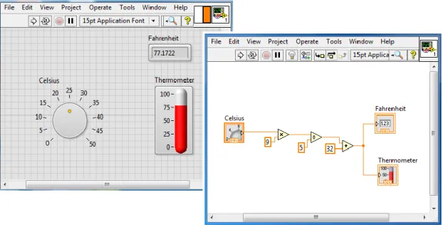
The navigation software will be programmed using LabVIEW. LabVIEW is a programming environment which uses a graphical notation called “G” (for graphical), connecting nodes and wires through which the data flows. LabVIEW programs are called Vis (Virtual Instruments) and consist of three parts: a front panel, a block diagram and a connector panel (Figure 4.1). The front panel of the program is the graphical user interface (GUI) and contains the input and output controls and indicators of the VI, allowing the user to supply and receive information from the system. When controls or indicators are placed on the front panel, a terminal is automatically placed on the block diagram.

The block diagram contains the graphical source code of the user interface. The objects on the front panel are represented as terminals on the block diagram. The terminals reflect the changes made to the front panel objects. Block diagrams include terminals, subVIs, functions, constants and structures which are connected by wires. SubVIs are smaller portions of code which can be called from within a VI. SubVIs are the same as Vis, consisting of a front panel and block diagram and are used for simplifying the main VI.

Figure 4.1 LabVIEW VI. Front panel (left), Block diagram (right)

The third art of a VI is the connector pane. The connector pane is needed when a VI is called as a subVI and appears in the top right-hand corner of every front panel next to the VI icon. The connector pane is a set of terminals that correspond to the controls and indicators of the VI (the inputs and outputs that are wired to the VI). The VI icon is the graphical representation of a VI and is what represents the VI on the block diagram when the VI is used as a subVI.

4.2 Robotics Simulator

The robotics simulator used for this project is the NI LabVIEW Robotics Module which is connected to the LabVIEW software. This module has a wide range of robots, sensors and environments, and there is also the option to design your own robot and environment with separate CAD software.

(37)

Chapter 4. Implementation using a Robotics Simulator

37 Before a new project is created, a window appears where the characteristics of the simulation must be defined. First an environment type is chosen, the type of environment must be suitable for the size and type of robot that will be used. Once a robot has also been chosen it usually has a sensor by default, but this can be removed and changed for a variety of other sensors.

4.2.1 Simulated Robot and Sensors

In this case the DaNI Starter Kit 1.0 has been used with a Hokuyo URG Series laser scanner, a Sparkfun Atomic 6DOF Inertial Measurement Unit (IMU) and a Honeywell HMC6343 compass module (Figure 4.2). Tests will be carried out in different simulation environments.

Figure 4.2 LabVIEW Robotics Simulator

The DaNI Starter Kit robot (Figure 4.3) is a differential drive robot based on a NI Single Board RIO controller. The NI Single Board RIO platform integrates a real-time processor, a reconfigurable FPGA and analogue and digital input/output. The robot moves by means of four wheels, controlled by two DC motors (right and left). Each motor has an optical encoder for odometry.

(38)

38

The laser scanner used for the simulation is a Hokuyo URG series (Figure 4.4). This laser has a scanning range from 0.02m to 5.6m, covering 240 degrees. The scan rate is 10Hz with a 1mm resolution and ±10mm accuracy. Normally around 250-350 readings are obtained with each scan, however, with the robotics simulator just 27 points are obtained.

Figure 4.4 Hokuyo Laser Scanner

The only IMU sensor available on the simulator is the Sparkfun 6DOF (Degrees of Freedom) IMU with consists of a 3-axis accelerometer, a dual axis pitch and roll gyroscope and a yaw-rate gyroscope (Figure 4.5). The accelerometer has a ±3g range and the gyroscopes have a scale of 300˚/s.

Figure 4.5 6DOF IMU

For orientation, a 3-axis compass module is used (Figure 4.6). This compass measures the magnetic distortion in heading pitch and roll directions. The precision for heading calculation is 2˚.

Figure 4.6 HMC6343 Compass Module

4.2.2 Simulator Environments

The algorithms implemented in this project will be tested in two different simulated environments. The first environment is designed especially for the DaNI Starter Kit robot (Figure 4.7).

(39)

39 The material of the ground and obstacles can be modified, in this case stone is used for the ground and the material for the obstacles is either stone, wood or plastic. The materials chosen are important as in real tests the robot will move differently on different surfaces and the precision of the sensors will vary slightly depending on the material of the obstacles.

Figure 4.7 Robot Scene Environment

The second environment used has been built using obstacles and modifying their size and properties. This environment consists of a stone flat ground base and wooden walls and obstacles to resemble rooms and doorways (Figure 4.8).

(40)

40

This could environment could also have been built by designing the environment using CAD software such as Solidworks and then importing the model to the simulator. For this project, the environment has been designed using the LabVIEW simulator as it is easier to modify the position and properties of the features.

4.3 Development of the Navigation Software

4.3.1 Initializing the Simulator, Robot and Sensors

The first part of the program is the initialization of the robot and sensors in the simulator. The simulation program consists of a manifest file, and ID List and the Vis. The manifest file is where the simulation environment and components are saved in an .xml file. The ID list is a text file which contains the ID names of the robots, components and obstacles in the environment.

Figure 4.9 Simulator Initialization

To initialize a robot in the simulator, the initialize simulator block for the robot must be connected to the error in from the simulator and the robot ID from the ID list must be defined as an input (Figure 4.9). If more than one robot is used in the same program, the robot ID differentiates them. The same must be done for each sensor, the robot ID and sensor ID must be defined. The simulator must be loaded and initialized before any other part of the program, otherwise there will be an error.

**4.3.2 Path Planning: A* Algorithm**

To implement the A* algorithm, an occupancy grid of the robot environment is needed. The precision of the map provided will influence the results of the algorithm. In an occupancy grid map, the first cell (0,0) is located at the bottom left corner of the grid. In LabVIEW, a matrix is defined with the first element in the top left corner, so when an occupancy grid is defined, the LabVIEW Create Occupancy Grid Map VI automatically adjusts the input matrix or file relative to the new origin.

The first occupancy grid defined as a matrix (with the origin (0,0) in the top left corner) for the robot scene environment is:

(41)

Chapter 4. Implementation using a Robotics Simulator 41 1 1 1 1 1 1 1 1 1 1 1 1 1 1 1 1 1 1 1 1 1 100 1 1 1 1 100 100 1 1 1 1 100 100 1 1 1 100 100 100 1 1 1 1 1 100 1 1 1 100 100 1 1 1 1 1 1 1 1 1 1 1 1 1 100 100 100 1 1 1 1 1 1 1 1 1 100 100 1 1 1 1 1 1 1 1 1 1 1 100 1 1 1 1 1 1 1 1 100 100 1 100 1 1 1 100 1 1 1 1 100 1 1 1 1 1 1 100 1 1 1 1 100 1 1 1 1 1 1 100 1 1 1 1 100 1 1 1 1 1 1 1 1 1

Figure 4.10 Robot scene rotated with origin in top left corner

The values in each cell are the cost for the robot to move to the cell. The obstacles have a cost of 100 and free space has a cost of 1. Other values could be used if a path is possible but not desired, for example, in the case of Google maps, backstreets would have a higher cost than motorways.

The total size of the environment (Figure 4.10) is 6 x 6 metres and the chosen size for each square in the grid is 0.5 x 0.5 metres. This size was chosen as the size of the robot is approximately 0.4m x 0.3m, if a smaller size were chosen the robot would occupy more than one square and the algorithm would not execute properly. The environment was divided into a grid of 12 x 12 cells. For the second environment, the same sized squares were used and a grid of 18 x 20 cells was obtained, with the origin in the top left corner (Figure 4.11).

(42)

42 1 1 1 1 1 1 1 1 1 1 1 1 1 1 1 1 1 1 1 1 1 1 1 1 1 100 1 1 1 1 1 1 1 1 1 1 1 1 1 1 1 1 1 100 1 1 1 1 1 1 1 1 1 100 1 1 1 1 1 1 1 100 1 1 1 1 1 1 1 1 1 100 1 1 100 1 1 1 1 100 1 1 1 1 1 1 1 1 1 100 1 1 1 1 1 1 1 100 1 1 1 1 1 1 1 1 1 100 1 1 1 1 1 1 1 100 1 1 1 1 1 1 1 1 1 100 1 1 1 1 1 1 1 100 1 1 1 1 1 1 1 1 1 100 100 100 1 1 100 100 100 100 1 1 1 1 1 1 1 1 1 100 1 1 1 1 1 1 1 100 1 1 1 1 1 1 1 1 1 100 1 1 1 1 1 1 1 100 1 1 1 1 1 1 1 1 1 100 1 1 1 1 100 1 1 1 1 1 1 1 1 1 1 1 1 1 1 1 1 1 1 1 1 1 1 1 1 1 1 1 1 1 1 1 1 1 1 1 1 1 1 100 1 1 1 1 1 1 1 1 1 100 1 1 1 1 1 1 1 100 1 1 1 1 1 1 1 1 1 100 1 1 1 1 1 1 1 100 1 1 1 1 1 1 1 1 1 100 1 1 1 1 1 1 1 100 1 1 1 1 1 1 1 1 1 100 1 1 1 1 1 1 1 100 1 1 1 1 1 1 1 1 1 100 100 100 100 100 1 1 100 100 100 100 100 100 100 100 1 1 100 100 1 1 1 1 1 1 1 1 1 1 1 1 1 1 1 1 1 1

Figure 4.11 Second robot environment rotated with origin in top left corner

The occupancy grid can be defined directly as an array in LabVIEW or can be written in a text file and converted to an array. For this program, the map has been written in a text file as it is easier to manage when there are many cells.

Once the occupancy grid map has been defined, the start and goal cells must be defined. The square number is the position in the matrix that the goal occupies, not the position in metres of the robot. All the data is then processed by the A* VI which calculates the path with the lowest

(43)

43 cost to reach the goal. This VI returns a set of path references which are then processed by the “Get Cells in Path VI”. The output of this VI is a list of cell coordinates (Figure 4.12).

Figure 4.12 A* Algorithm in LabVIEW

4.3.3 Robot Motor Velocity Control

To control the movement of the robot a steering frame is used. The steering frame converts the centre robot velocity to the individual left and right wheel angular velocities. In the steering frame, the geometry of the robot and steering type is defined and the formulas explained in the previous chapter are used. For the DaNI robot, a steering frame is already available (Figure 4.13). The maximum forward and angular velocities and the direction the motor turns in are defined, as well as the geometrical parameters such as the distance between the wheels, wheel size and type, etc.

Figure 4.13 Steering frame for DaNI robot

The steering frame input is a 1D array of the forward velocity, lateral velocity and angular velocity. For a differential robot, the lateral velocity will always be 0. The output of the steering frame is an array of the left and right wheel velocities. These velocities are then sent to the “Write Motor Velocity Setpoints VI”.

In the same way that the velocities are written, the estimated wheel velocities can be obtained from the wheel encoders. These can be converted back to the forward and angular centre velocities of the robot by the steering frame “Get Velocity from Motors VI”.

(44)

44

4.3.4 Localization: Dead Reckoning

Dead Reckoning consists in determining the position of the robot from the encoders by measuring the distance travelled. The uncertainty of dead reckoning increases over time and distance.

The change in heading is obtained by integrating the angular velocity, ω. The sampling interval dt is 20ms which is the time between each iteration of the while loop. This difference in heading is added to the initial angle to obtain an estimation of the current heading.

𝜃 = 𝜃0+ ∫ 𝜔 𝑑𝑡

To obtain the x and y coordinates, the velocities in the forward and lateral direction are rotated by the difference in angle. These rotated velocities Vx’ and Vy’ are then integrated to obtain the

new position. The time interval dt is the time between each iteration of the while loop. The new position is the sum of the initial position and the change in x and y coordinates.

𝑥 = 𝑥0+ ∫ 𝑉𝑥′ 𝑑𝑡

𝑦 = 𝑦₀+ ∫ 𝑉_𝑦′_𝑑𝑡

The estimated position of the robot is shown on the user interface and is compared to the actual position of the robot.

The actual position of the robot can be obtained by the “Get Simulator Reference VI” when using the robot simulator. With this VI it is possible to ask the robot its exact position in Cartesian coordinates, the velocity and angular velocity among other variables (Figure 4.14).

Figure 4.14 Simulated robot real position and heading

4.3.5 Obstacle Avoidance: Vector Field Histogram Algorithm

To obtain better results from the A* algorithm, it has been combined with a local navigation algorithm. If the robot environment is only partially mapped, there could be obstacles in the original planned path which are unknown to the robot.

There are two vector field histogram (VFH) Vis available in LabVIEW, a basic VI for obstacle avoidance, and an Advanced VFH VI for when the robot must also reach a goal. The Advanced VFH has been used with the coordinates previously obtained from the A* algorithm as sub-goals.

(45)

45 Figure 4.15 Advanced VFH VI

The inputs to the Advanced VFH VI are:

- The obstacle clearance distance is the minimum distance by which the centre of the robot can approach an obstacle. The obstacle clearance distance and threshold distances are controls on the front panel and are defined by the user.

- The heading is an input of two angles: The current heading of the robot and the direction at which the goal position lies (target heading). The current heading is obtained directly from the compass sensor. The target heading is calculated from the position obtained by dead reckoning with the encoders. The heading is calculated by subtracting the current x and y coordinates from the goal coordinates and applying the 2-input inverse tangent to obtain the angle to the goal position.

- Distances are the measurements obtained from the LiDAR sensor and are the distances to obstacles.

- Direction angles are the angles in radians at which objects are located and correspond to the distances. These are also given by the LiDAR sensor.

- Thresholds specify how close an object must be to be considered an obstacle and when an obstacle is considered too close to clear. This cluster contains the inner threshold distance (distance from obstacle at which a direction is considered blocked) and the outer threshold distance (distance to an obstacle at which the direction is no longer considered blocked). These parameters are defined by the user on the user interface. - # bins are the number of headings the VI considers for travelling. To get the best results,

a smaller number of headings than is possible should be used. The best results have been obtained on the simulator with a #bins of 24 with 27 LiDAR readings. This variable is also defied by the user on the user interface.

- The maximum heading change is the greatest angle that the robot can change direction by when a path is blocked. Although it is possible for the robot to turn 90 degrees or more, the best results were attained with this parameter set to 85 degrees.

The outputs from the VFH VI are:

- The chosen heading is the heading calculated by the vector field histogram as the best direction of travel with respect to the goal position and the obstacles in the environment.