Eric G.A. Gaury
1)2)y
Jack P.C. Kleijnen
1)y
Henri Pierreval
2) 1)Department of Information Systems and CentER, Tilburg University, Postbox 90153, 5000 LE Tilburg, The Netherlands
2)
Laboratoire d’Informatique, de Modélisation et d’Optimisation des Systèmes,
Equipe de Recherche en Systèmes de Production de l’Institut Français de Mécanique Avancée, IFMA, B.P. 265, F-63175 Aubière Cedex, France
Traditionally pull production systems are managed through classic control systems such as Kanban, Conwip, or Base stock, but this paper proposes ‘customized’ pull control. Customization means that a given production line is managed through a pull control system that in principle connects each stage of that line with each preceding stage; optimization of the corresponding simulation model, however, shows which of these potential control loops are actually implemented. This novel approach may result in one of the classic systems, but it may also be another type: (1) the total line may be decomposed into several segments, each with its own classic control system (e.g., segment 1 with Kanban, segment 2 with Conwip); (2) the total line or segments may combine different classic systems; (3) the line may be controlled through a new type of system. These different pull systems are found when applying the new approach to a set of twelve production lines. These lines are configured through the application of a statistical (Plackett-Burman) design with ten factors that characterize production lines (such as line length, demand variability, and machine breakdowns).
(Pull Production / Inventory; Sampling; Optimization; Evolutionary Algorithm) JEL classification: C0
1. Introduction
Much research has already been performed in the field of production control and inventory management. Production control has a major influence on the performance of a manufacturing company, notably in terms of inventory, production delays, and makespan. Thus, the competitiveness
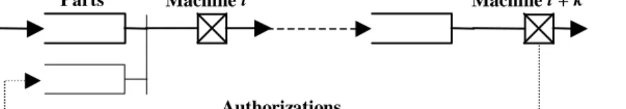
Figure 1 Pull principle illustrated through a simple line of queues
Machine i Parts Authorizations Machine i + k Part flow Information flow Legend:
of a company relies partly on its production control strategy. There are two general types of strategy: push control and pull control. The former has a production plan made according to estimates for demand and lead-time. The latter uses demand occurrences to control production. This paper focuses on pull control applied to production lines processing a single part type. In such a system, a workstation can produce if and only if the workstation is idle and an authorization (e.g., a card or Kanban) is available. An authorization originates from a workstation downstream in the production line, when a part is removed from its input inventory; see Figure 1 for a simple illustration. The number of authorizations circulating between machines i and i + k determines the maximum Work In Process (WIP) between these two stages.
Kimura and Terada (1981) claim that the multiple objectives of a pull system are to minimize WIP's average and fluctuations, shorten production lead-time, prevent amplified transmission of demand fluctuations from stage to stage, enhance control through decentralization, react faster to demand changes, and reduce defects. These objectives explain why pull production has received such a growing interest from both companies and researchers, after its formalization at the end of the 1950s.
Pull systems can be specified by the way demand information flows through the production system. Gstettner and Kuhn (1996) identified three basic pull systems, namely Kanban, Conwip, and Base stock; they also considered the serial combination of these pull systems within a production line. In the next section, we describe these three basic systems and their possible serial combinations; we call these combinations, segmented systems; we also consider joint systems, that is, combinations of control systems on the same segment of a production system. In section 3 we propose 'customized' pull control. Customization means that a given production line is managed through a pull control system that in principle connects each stage of that particular line with each preceding stage; optimization, however, shows which of these potential control loops are actually implemented. In section 4 we define a set of twelve production lines, which are compatible with models found in the literature on pull systems. Section 5 describes the solutions obtained when applying our customization to the set of lines. In section 6 we analyze these solutions, and propose new structures of pull control that generalize our results.
2. Pull production control systems
2.1. Three basic pull systems
(i) Kanban
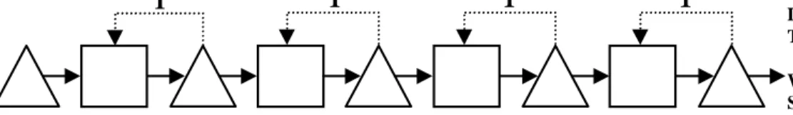
Dr. Taichi Ohno, manager at the Toyota Motors company, has developed the Kanban strategy. The principle is to limit the inventory level at each stage of a process, by defining control loops between each pair of consecutive stages (Monden, 1993); see figure 2. Cards materialize authorizations, but
there are many implementation forms of Kanban. Indeed, several papers propose adaptations of the original strategy. Berkley (1992) proposes a classification of Kanban system models; he uses operational design criteria such as the blocking mechanism, the withdrawal strategy, and the type of Kanban cards. Huang and Kusiak (1996) survey various Kanban systems and alternatives, and classify the previous studies. Chu and Shih (1992) compare numerous simulation studies on Just-In-Time (JIT) production systems. Price, Gravel, and Nsakanda (1994) review optimization models of Kanban systems. Sing and Brar (1992) classify various models. Gaury, Pierreval, and Kleijnen (1997) take stock of the way modeling techniques and simulation are used to study Kanban systems.
The benefits that Japanese companies obtained through the Kanban method were reported to be important, so researchers tried to compare the Kanban method with classical methods such as Material Requirement Planning (MRP), order point systems, and other push-type systems. These studies agree on one fact: a Kanban system is very efficient in an ideal environment, that is, an environment with low process and demand variability, few breakdowns, etc. In a typical Western environment, however, the Kanban method is much less efficient. Some studies even conclude that in such an environment push systems perform better than pull systems. Huang, Rees, and Taylor (1983) emphasize that high production rates can be realized only when the number of Kanban is chosen optimally. Thus, even in unfavorable environments, optimized Kanban systems may perform almost as well as push systems, in terms of output, but with a WIP level always lower in terms of average and variability.
(ii) Conwip
Conwip stands for Constant Work In Progress. Spearman, Woodruff, and Hopp (1990) proposed the name Conwip, but Bertrand (1983) proposed a similar approach under the name of workload control. Both approaches can be considered as capacity-based order review/release (ORR) strategies; see Philipoom and Fry (1992) for a short review of ORR strategies.
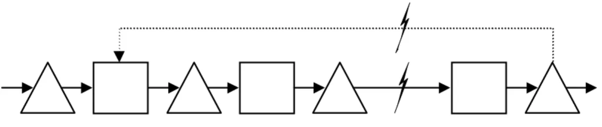
The objective of Conwip is to combine the low inventory levels of Kanban with the high throughput of Push. One way to achieve this objective is to consider a Push system that has only a limited number of parts allowed into it: raw materials can be released into the system only when the last stage asks for it (Pull principle). This limitation is implemented through a single control loop that
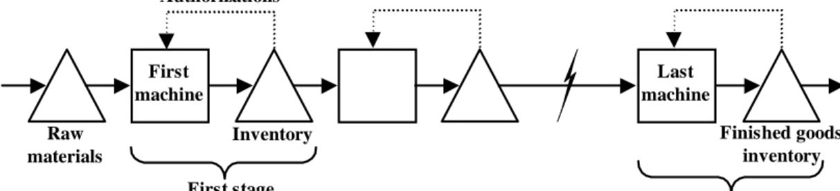
Figure 2 Kanban system
Raw materials
Inventory Finished goods
inventory Authorizations First stage First machine Last machine Last stage
links the last stage to the first one. Within the system, each stage can produce as fast as it can (Push principle). Similarly, workload control is an order release strategy that aims at maintaining a specific workload level of the production system. Comparing figures 2 and 3 shows that Conwip's implementation is much simpler than Kanban's: there are fewer control loops. Thus, modeling and optimization are easier. Actually, a Conwip system can be viewed as a Kanban system with a single loop that controls the whole production line.
Roderick, Phillips, and Hogg (1992) and Roderick, Toland, and Rodriguez (1994) compare Conwip with MRP and three order release strategies. They conclude that Conwip gives the best performance measured in mean WIP, mean throughput, and proportion of tardy jobs. Therefore, Roderick et al. (1992) recommend Conwip as a 'strategy that should be seriously considered by practitioners for implementation in actual shop environments'. De Koster and Wijngaard (1989) compare the performance of local control (Kanban) and integral control (workload control and base stock) for production lines. They did not find any significant difference in performance between these types of control.
(iii) Base stock
There are several definitions of base stock. This policy was developed in the 1950s, and has been extensively used by practitioners ever since. Bonvik, Couch and Gershwin (1998) and Lee and Zipkin (1992) consider the base stock policy described in Kimball (1988); see figure 4. Each stage of the production line holds an initial amount of inventory Si, called the base stock level. Any demand for
finished products immediately triggers demands at each preceding stage: demand information is broadcasted from the last stage to each stage in the production line. Demands that cannot be filled from stock, are backordered. There is no upper bound for the inventory level at each stage. The base stock levels Si are the only parameters of the base stock policy.
An advantage of base stock is its responsiveness to demand: as soon as a demand occurs, all the stages can start working simultaneously. A drawback, however, is that consecutive stages are not
Figure 3 The Conwip strategy
Figure 4 Base stock strategy
coordinated: if one stage fails, preceding stages do not stop working. A solution is to limit the amount of inventory, using authorizations as in Kanban. When a finished good is delivered, one card is sent to each stage of the production line, thereby allowing stages to produce. Such a system is called an
Integral Control System; see Buzacott and Shanthikumar (1993).
2.2. Segmented systems
The three basic pull systems (described in section 2.1) can be combined along a production line. The idea is to segment the production system into cells, and use a specific control strategy per cell. This is a recent approach, and much research remains to be done. The main issues concern the definition of cells and the configuration of the control strategy per cell.
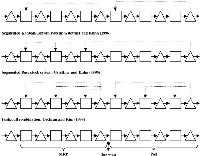
Figure 5 shows a variety of segmented control systems, introduced in the literature. Ettl and Schwehm (1994) and Di Mascolo, Frein, and Dallery (1996) consider Kanban systems with each loop controlling a set of machines. Such systems can be viewed as segmented Conwip systems. Gstettner and Kuhn (1996) propose segmented Kanban/Conwip and Base stock systems, but they do not study such systems nor do they propose a design procedure. Segmented push/pull systems have also been
Figure 5 Segmented systems in the literature
Segmented Conwip system: Ettl and Schwehm (1994) and Di Mascolo, Frein, and Dallery (1996)
Segmented Kanban/Conwip system: Gstettner and Kuhn (1996)
Segmented Base stock system: Gstettner and Kuhn (1996)
MRP Junction Pull
point Push/pull combination: Cochran and Kim (1998)
investigated. For instance, Cochran and Kim (1998) consider a production line that is controlled partly through MRP and partly through a pull strategy; they use simulated annealing to optimize inventory levels and the junction point, which separates the production line into two subsystems. Olhager and Ostlund (1990) emphasize that the junction point can be the customer order point, a bottleneck resource, or a point derived from the product structure.
2.3. Joint systems
Control mechanisms can also be combined to control the same part of a system: superimpose several control systems, in order to obtain their respective benefits. The main issue is to evaluate the performance of the new systems, relatively to other control strategies. Such comparisons should not be limited to pure performance: it should also include issues such as implementation complexity (obviously, Conwip is simplest). One aspect of complexity is the control strategy's number of parameters (such as number of cards, base stock levels) compared with the number of stages of the production system (say) N. Kanban and Base stock both have N parameters, whereas Conwip has only one parameter (so, Conwip's complexity is independent of the number of stages).
Bonvik et al. (1998) propose a control system called (two-boundary) Hybrid that combines local control using Kanban, and integral control using Conwip; see figure 6. Hybrid performs better than Base Stock, Kanban, Conwip, and Minimal Blocking (variation of Kanban), not only in terms of average overall inventory and service level but also in robustness to demand rate changes. As for complexity, Hybrid is easy to implement as a modification of Kanban; its number of parameters is N.
Buzacott (1989) and Zipkin (1989) propose Generalized Kanban, which combines Base stock and Kanban. The objective is to associate Base stock's rapid reaction to demand and the initial amounts of inventory with Kanban's coordination between consecutive stages and local control of inventory; see figure 7. A general approach to Base stock/Kanban joint systems is proposed in Dallery and
Figure 6 Kanban/Conwip Hybrid
Figure 7 Joint Kanban/Base stock systems
Liberopoulos (1995). The resulting system is called Extended Kanban control system. It has the same objective as Generalized Kanban, but is claimed to be conceptually clearer and potentially easier to implement. Both systems, however, are rather complex since they both have 2N parameters. Liberopoulos and Dallery (1997) propose variations of Extended Kanban for various production environments.
This short review of the literature on pull control shows that researchers have improved pull production control systems over the years. By combining existing control systems, they have created more efficient systems. However, there is a limit to this approach since it is based on three basic systems and almost all possible combinations have already been investigated. Yet, it is possible to imagine information flows that cannot be obtained with simple combinations of the three basic systems. Therefore, we propose a new approach that investigates such control systems.
3.
Customized pull production control system
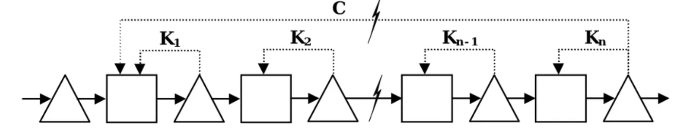
Gaury, Kleijnen, and Pierreval (1997) propose a methodology for choosing among Kanban, Conwip, and Hybrid. The idea is to optimize a generic system that aggregates the information flows of the three systems; see figure 8. Thus, the generic pull system can model a Kanban, a Conwip, or a Hybrid system, depending on the choice of the various parameters; see table 1. A control loop with an infinite number of authorizations does not impose any constraint on the flow of parts. Such a loop has no effect on the performance of the production line, so it can be removed from the generic system; it does not need to be implemented. For a given production system, the optimal configuration of the generic system not only shows which type of pull strategy is preferred, but also which values should be selected for the various numbers of cards. Suppose that for the example of a four-stage production line, optimization of the generic model gives k1 = 2, k2 = 3, k3 = 5, k4 = 4, and c = ∞. According to
table 1, this configuration of the generic model is equivalent to a Kanban system. Thus, Kanban provides the best performance; its optimal configuration is k1 = 2, k2 = 3, k3 = 5, and k4 = 4.
Table 1 Generic system for three pull production control systems
C K1 K2 ... Kn - 1 Kn Kanban ∞ k1 k2 ... kn - 1 kn
Conwip C ∞ ∞ ... ∞ ∞
Hybrid C k1 k2 ... kn - 1 ∞
Figure 8 The generic model for Kanban, Conwip and Hybrid in Gaury et al. (1997)
K
1K
2K
n - 1K
nGaury, Pierreval, and Kleijnen (1998) use an evolutionary algorithm to optimize the generic model for a production line with four stages inspired by a Toyota factory. They conclude that the resulting system cannot be classified as Kanban, Conwip, or Hybrid; it may be considered to be a simplified Hybrid system. In general, the best solution found through the optimization of the generic model does not necessarily correspond to any predefined system.
Huang and Kusiak (1998) criticize predefined strategies such as Kanban, for not considering the specific characteristics of manufacturing systems. They propose an algorithm based on decision rules for choosing which strategy (push or pull) should be adopted at each stage of a manufacturing system. Even though they consider only local control (no combination), they are the first to investigate what we call customized control systems: each production system has its own specificity and requires a special control system; predefined systems (such as Kanban and Conwip) might not be good enough.
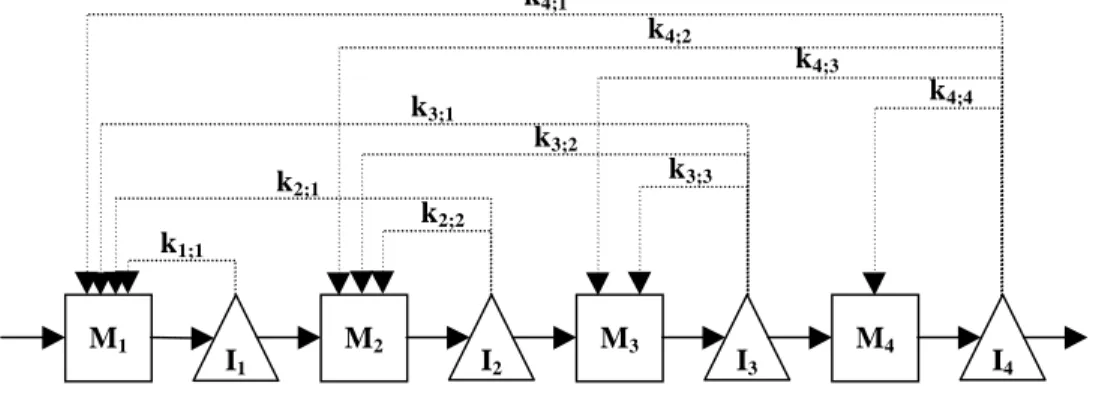
Our objective is to design a pull production control system for a given production system, without using any predefined type of pull system a priori. Instead, we search for a control system in the whole set of possible pull systems, including local and integral control, segmented and joint systems. For this purpose we design a new generic system that accounts for all possible types of pull production control systems: through control loops we link each stage to all its preceding stages. Figure 9 shows this new generic system for a production line with four stages, where ki; j denotes the number of
authorizations circulating in the loop linking stage i to stage j, Mi and Ii denote respectively the
machine and the inventory at stage i. There are 4(4 + 1)/2 = 10 loops. As in the former generic model (Gaury et al., 1997), we do not implement a control loop with an infinite number of authorizations. A major difference, however, is that the former generic model was limited to Kanban, Conwip, and Hybrid.
Let us consider a general production line with N stages. If we want the generic model in figure 9 (N = 4) to be a Kanban system, then we select the numbers of authorizations as follows: ki; j = ∞, ∀(i, j) ∈ {1...N}2 / i ≠ j (meaning: ki; j has an infinite value for all i and j such that i ≠ j), and ki; i << ∞, ∀i ∈ {1...N} (meaning: ki; i has a finite value for all i). Similarly, Conwip is obtained by choosing kN; 1 << ∞, and ki; j = ∞, ∀(i, j) ∈ {1...N}
2
/ (i, j) ≠ (N, 1). The generic model cannot represent the Base stock strategy of section 2.1 because that strategy uses information about demand occurrences, whereas the generic model focuses on information about actual deliveries. The Integral Control (variant of Base stock; see section 2.1.iii), however, is a possible instantiation of the generic model. Also, the generic model can represent control systems that have not been investigated in the literature. For instance, one can imagine a system for which control loops link each machine to the first one; this system requires authorizations from all machines to release raw materials.
Hence, we can use the generic system of figure 9 to find the best pull production control system for a given production system. Indeed, optimizing the various authorization numbers ki; i in this generic
loops must be implemented. The advantage of our approach is that we do not try to apply any predefined type of systems. This advantage, however, seems costly in terms of complexity. For a production line with N machines, the optimization model contains N (N + 1)/2 control loops. Thus, the optimization procedure has to deal with a rather large search space. For instance, for ten machines, the optimization model has 55 control loops. If the various authorization numbers are chosen from {1…20} ∪ {∞}, then the search space includes 2155 = 5.27 x 1072 configurations of the generic system. Obviously, it does not seem reasonable to attempt solving the exact optimization problem for large systems. Instead, our objective is to derive rules that can be generalized to larger systems. In this paper we choose to select a sample of simple line configurations for which the generic model will be configured and optimized. In the next section we define a sample of production lines compatible with models studied in the literature.
4.
A sample of twelve production lines
In order to build a sample of production lines, we analyze the characteristics of pull production systems (mainly Kanban) studied in the literature. This analysis yields a list of ten factors, with typical values. We define three factor classes: process, demand, and performance. Below, we discuss each class individual factors, and their values used in the literature; for each factor we choose two values or levels.
4.1.Process factors
Line length or number of stages
Chu and Shih (1992) point out that most of the Kanban models in the literature are relatively small. Actually, Krajewski, King, Ritzman, and Wong (1987) study a 50-stage manufacturing system, but the usual length of the modeled lines is four or five stages, and the largest is nine. Because Conwip models are simpler, they can easily be studied for large production systems. Table 2 gives some references for the line length factor. For our sample of production lines we choose two levels: a low level of four stages, and a high level of eight stages.
Figure 9 Generic system accounting for all possible pull patterns
k3;3 k4;4 k4;3 k4;1 M1 M2 M3 M4 I1 I2 I3 I4 k4;2 k3;1 k3;2 k2;1 k2;2 k1;1
Table 2 Line length in the pull literature
Reference Control system Line length
Krajewski et al. (1987) Kanban 50
Sarker and Fitzsimmons (1989) Kanban 9
Spearman et al. (1990) Conwip 10
Meral and Erkip (1991) Kanban 3, 4, 5, and 6 Savsar and Al-Jawini (1995) Kanban 3, 5, and 7 Bonvik et al. (1997) Kanban, Conwip, Hybrid, Base stock 4 Line imbalance
A production line is said to be non-balanced (bottlenecked) when resources do not have the same production rate. Sarker and Harris (1988) and Gupta and Gupta (1989) claim that balanced pull systems outperform non-balanced ones. The literature, however, does not agree on this point: for instance, Villeda, Dudek, and Smith (1988) show that some imbalance patterns can improve output rates.
A production line can be non-balanced in several ways. (i) The mean processing times in different stages can differ. This form of imbalance is studied most often. Various patterns are defined and analyzed; for example, bowl (the machines at the two ends of the line have the highest mean processing times), funnel (mean processing times are getting shorter from stage to stage), and reversed funnel (mean processing times are getting longer from stage to stage); see Hillier and Boling (1966). (ii) A line can also be non-balanced in its processing time variances, and its machine breakdown rates. Thus, the imbalance factor is very complex. We focus on the mean processing times: because process variability and machine reliability will be considered as factors, the other forms of imbalance will also be studied indirectly. We refer to Opwell and Pyke (1998) for an analysis of imbalance in both processing time means and variances in assembly systems.
Meral and Erkip (1991) define an interesting measure of imbalance in mean processing times: the Degree of Imbalance (DI) of a line is DI = max{TWC/N - min(PTi); max(PTi) - TWC/N}.N/TWC,
where PTi is the mean Processing Time at workstation i in an N-station line, and TWC/N is the mean processing time at a workstation on the balanced N-station line. Table 3 reviews some of the values for imbalance in the Kanban literature.
Table 3 Degree of imbalance in the Kanban literature
Reference DI
Villeda et al. (1988) 0 to 1.4 (step 0.2) 0 to 0.7 (step 0.1) Meral and Erkip (1991) 0, 0.1, 0.2, 0.45 Yavuz and Satir (1995) 0, 0.1, 0.3, 0.5
DI, however, does not account for the imbalance pattern (bowl, funnel, reversed funnel). Meral
and Erkip (1991) and Yavuz and Satir (1995) study the bowl phenomenon. For our sample of production lines, we define two factors, one for DI, and one for the imbalance pattern. The levels of the DI factor are 0 (a perfectly balanced line) and 0.5. For the latter DI level, the two imbalance
patterns are funnel and reversed funnel; we see the bowl pattern as a combination of funnel and reversed funnel, so we do not study bowl. The bottleneck will be the first or last resource in four stage lines, and the third or sixth resource in eight stage lines; see section 5.
Processing time variability
It is well known that performance is sensitive to processing time variability: inventory has to be raised in order to maintain acceptable service. The variance by itself does not fully characterize the variability of processing times: it has to be considered together with the mean. Thus, as a measure of variability we use the Coefficient of Variation (CV) defined as the standard deviation divided by the mean. Table 4 gives a review of CVs used in the study of Kanban systems. For our sample, we use a low level of 0.1 and a high level of 0.5.
Table 4 Coefficient of Variation of processing times in the Kanban literature
Reference Coefficients of variation, CV Sarker and Fitzsimmons (1989) 0, 0.1, 0.2, 0.3, 0.4, 0.6, 0.8, 1.0 Meral and Erkip (1991) 1, 1.5, 2
Swinehart and Blackstone (1991) 0.2, 0.5, 1.0 Savsar and Al-Jawini (1995) 0.2, 0.6, 1.2, 1.8 Yavuz and Satir (1995) 0, 0.1, 0.5, 0.9 Machine reliability
Two random variables are needed to model machine breakdowns: Time Between Failures (TBF) and Time To Repair (TTR). Many different distributions have been used in the literature, often without justification. Table 5 reviews distributions in the Kanban literature. Yavuz and Satir (1995) use a maintenance model instead of a reliability model: they model a policy of preventive maintenance. Preventive maintenance should be widely used in companies. Practice, however, is often different. Therefore, we consider a reliability model rather than a maintenance model. For the time between failures we use a popular distribution, namely the exponential, in order to make comparisons with previous literature. Time to repair is not really predictable: it can be very short, but also extremely long. An exponential distribution is then appropriate. We define two levels for the machine reliability factor: first we assume that the machines are perfectly reliable; next we generate TBF and TTR through exponential distributions.
Table 5 Machine breakdowns in the Kanban literature
Reference TBF Distribution TTR Distribution Krajewski et al. (1987) Normal Normal So and Pinault (1988) Exponential Exponential Sarker and Fitzsimmons (1989) Normal Exponential Wang and Wang (1990) Exponential Exponential Yavuz and Satir (1995) Uniform Uniform Bonvik et al. (1997) Exponential Exponential
4.2.Demand factors
Demand rate
In a production system the demand rate may change frequently (this happens more often, since the design of new products requires less time). So it is a key issue to know whether the choice of a control system depends on the demand rate: once a control system is implemented, it might not be changed easily. In order to have real meaning, the demand rate has to be defined relatively to line capacity: define the ratio of demand rate and long-term capacity of the line. We select two levels: a low level of 0.8, and a high level of 0.9.
Demand variability
For demand variability we use the same principle as for processing time variability: we take CV. A sample of values in studies on pull control systems is given in table 6.
Table 6 Demand variability in the Kanban literature
Reference Demand CV
Berkley (1996) 0.1, 0.045 Yavuz and Satir (1995) 0.052, 0.075, 0.115, 0.133 Savsar and Al-Jawini (1995) 0, 0.1, 0.316, 0.447, 0.707, 1
Next, we choose two levels: CV = 0, and CV = 0.5. The case CV = 0 may correspond to dependent demand (internal customers); in Bonvik et al. (1997), for instance, the production line feeds an assembly system, which processes parts at a constant rate.
Customers' attitude
We define customers' attitude as willingness to wait for finished products. We consider two extreme cases. In the first one customers do not accept to wait at all, and do not order if they cannot be satisfied from stock: lost sales scenario. In the second case, customers are always willing to wait, and orders that cannot be filled from stock are backlogged: backorders scenario. Most publications on pull production consider the backorders scenario. Bonvik et al. (1997), however, use the lost sales scenario.
4.3.Performance factors
Chu and Shih (1992) identify three performance measures frequently used in the Just-In-Time literature: facility utilization, output rate, and WIP. Goldrat and Fox (1986), however, argue that facility utilization should not be considered as a performance measure, since the goal of a production system is not to keep resources (workers and machines) busy. Output rate should be measured relatively to demand rate: a production system should not overproduce; yet it should meet demand requirements on time. Thus, we use the proportion of demand actually met from stock as one performance criterion. We also use a weighted sum of the average WIP levels along the line.
Targeted service level
The service level (also called fill rate) is the proportion of demand supplied from stock. Intuition tells that the higher the level of finished good products, the higher the service level. Thus, the choice of a target value for the service level affects the overall WIP amount. The service level should be set by managers. It may vary from one production system to another, so it is necessary to consider the service level as a factor (not only as a performance measure). Service level targets close to 100% may be used for systems with lost sales, whereas lower targets correspond to systems with backorders. Setting a target for the service level has not often been done in the literature; yet, Bonvik et al. (1997) do use a target, namely 99.9%. We will also use service levels close to 100%: a low level of 95% and a high level of 99%.
Inventory value (added value)
An objective of pull production is to minimize inventory levels. Thus, the inventory level is a major performance indicator. In some cases, however, managers may need to account for the value of inventory. Indeed, whereas keeping a high finished good inventory may be good for the service level, it may be prohibitive in terms of cost. Goldrat and Fox (1986) emphasize that inventory is invested money; improved competitiveness can be achieved by minimizing this investment.
We use the total value of inventory as a performance measure. After each operation, the value of a part increases. We assume that this added value is the same at each stage, and we define the total value factor as the ratio of the finished good value and the raw material value. We choose two levels: 1.0 (value not of interest to managers; total inventory value is equal to total amount of inventory) and 2.0. We expect these two cases to yield different inventory allocations along the production line, and also different information flows.
4.4.Summary of factors and levels
Table 7 gives an overview of our ten factors, now labeled from A through J, and their levels. A sample of line configurations can now be built through Design Of Experiment (DOE), which combines the various factor levels (see Kleijnen 1998 for an introduction to DOE in simulation). In order to minimize the number of combinations (configurations), we use the Plackett-Burman design (see Kleijnen, 1987 p. 329-336) displayed in table 8.
Table 7 Design factors and levels
Factor Level Letter
+
-Line length 4 8 A
Line imbalance 0 0.5 B
Imbalance pattern Funnel Reversed funnel C
Processing time CV 0.1 0.5 D
Machine reliability Perfect Breakdowns E
Demand CV 0 0.5 F
Demand rate/capacity 0.9 0.8 G
Service level target (%) 99 95 H
Inventory value ratio 1 2 I
Customers' attitude Lost sales backorders J
Table 8 Sample of production lines configurations, using Plackett-Burman design
Factors Line # A B C D E F G H I J 1 + + - + + + - - - + 2 + - + + + - - - + -3 - + + + - - - + - + 4 + + + - - - + - + + 5 + + - - - + - + + -6 + - - - + - + + - + 7 - - - + - + + - + + 8 - - + - + + - + + + 9 - + - + + - + + + -10 + - + + - + + + - -11 - + + - + + + - - -12 - - -
-Many of the factors selected to define a line configuration, are variability sources with specific probability distributions. Thus, it may be difficult to perform analytic studies on most of the twelve configurations specified in table 8. Therefore we choose simulation for the performance evaluation of these production lines. The next step is to determine the optimal configuration of the generic pull control system for each production line; we use a heuristic optimization procedure based on an evolutionary algorithm (EA). Other optimization techniques have been used to configure pull systems: simulated annealing (Chang and Yih, 1994), RSM (Davis and Stubitz, 1987), neural networks (Hurion, 1997), and exhaustive search in a restricted search space (Duri, 1997; Bonvik et al., 1997). An advantage of EAs, however, is that infinity can be used as an explicit value for the card numbers. We refer to appendix A for details about this optimization procedure.
5.
Simulation experiments
To evaluate the performance of the generic control system, we built twelve models corresponding to the twelve production lines in table 8. We use the SIMAN simulation language; see Pegden, Shannon, and Sadowski (1991). We estimate performance measures through single-run simulations, each with 240,000 time units, after eliminating a transient period of 10,000 time units.
The search space of the optimization procedures has 2110 and 2136 (21 is the number of integer values including infinity for kI; j, 10 and 36 are the number of loops) possible solutions for four- and
eight-stage production lines respectively, except for line #11, for which the search space has to be widened (the optimal number of Conwip cards is 27). Solutions may be simplified using a simple procedure: we measure the WIP level within each portion of the line controlled through a loop; if the maximal WIP level is below the corresponding number of cards, then the control loop does not have to be implemented. Conwip will be the reference for discussing our results because Conwip is the simplest strategy and it has proven to be very efficient. We find the optimal number of Conwip cards by running the simulation models for values chosen by dichotomy. Next we discuss the results for the first four line configurations. Other results are detailed in appendix B.
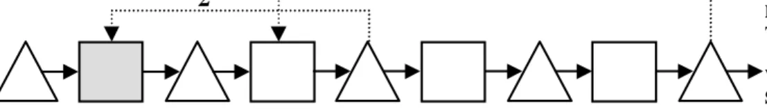
Line configuration #1
Surprisingly, the best control system found by the EA is a Kanban system; see figure 11. An interesting characteristic of our solution is that each control loop has only one card. Thus, manufacturing is highly synchronized: as soon as a machine stops, the machines upstream are not authorized to produce anymore and the machines downstream starve. The advantage is that inventory is extremely low. Such a system, however, is highly sensitive to variations (demand, process variability, breakdowns, etc). In fact, it is well known that there can be a single Kanban card per control loop if the production environment is ideal. Indeed, Monden (1983) and Sugimori, Kusunoki, Cho, and Uchikawa (1977) reported that Japanese managers use the following formula to determine the number of Kanban: yi≥ DiLi(1 + αi)/a, where yi is the number of Kanban at stage i, Di is the
average demand per time unit at stage i, Li is the average production lead-time at i, αi is a variable for
safety stock at i, and a is the container capacity (a single Kanban is attached to each container). If demand is met with probability one, then DiLi = 1. If there is no variation, then safety stocks are not
needed, so αi = 0. Moreover, if transport and switchover costs are unimportant, then there is no need
for containers so a = 1. Thus, in an ideal production environment, the minimum number of Kanban at each stage is one: yi≥ 1. In line configuration #1, demand is indeed constant, processing time
Figure 11 Line configuration #1 and best solution
1 1 1 1 STAGE 1 Processing times: Logn(1.0, 0.1) Breakdowns: TBF exp(1000) TTR exp(3) Value of inventory per unit: 1.0 STAGE 2 Processing times: Logn(1.0, 0.1) Breakdowns: TBF exp(1000) TTR exp(3) Value of inventory per unit: 1.333 STAGE 3 Processing times: Logn(1.0, 0.1) Breakdowns: TBF exp(1000) TTR exp(3) Value of inventory per unit: 1.666 STAGE 4 Processing times: Logn(1.0, 0.1) Breakdowns: TBF exp(1000) TTR exp(3) Value of inventory per unit: 2.0 DEMANDS Time between: 1.25 (constant) Workload: 80% Service target: 95% Lost sales
variability is low, and customer pressure is low (service level of 95% and no backlog); see table 7 and line 1 of table 8. Thus, it seems reasonable to have a single Kanban per loop.
For this line configuration, the best Conwip system has four cards, which is as many as the total in the best generic system. However, the performance of the Conwip system is not as good in terms of average inventory value: see table 9. The WIP allocation shows that Conwip pushes inventory to the end of the line, whereas Kanban guarantees a uniform allocation along the line. Since the value of inventory is increasing along the line, Conwip is relatively expensive. However, we note that Conwip yields the same average overall inventory level, but with a higher service level and simpler implementation. Thus, if the inventory value is not an important issue, then Conwip is preferred.
Table 9 Performance of the best Generic and Conwip systems for line configuration #1
Service WIP allocation Value Target is 95% 1 2 3 4
Kanban 1,1,1,1 5.997 98.91% 1 1 1 1 Conwip 4 6.38 100.00% 0.80 0.81 0.81 1.57
Line configuration #2
Line configuration #2 and the best control system found by the EA are shown in figure 12. This is a simple control system: only two control loops. It is also a new type of pull system, in the sense that it is neither a segmented nor a joint system. The tradeoff between service and inventory is as follows: the first machine is the bottleneck, but it is quick enough to satisfy more than 95% of demands; see table 10. Thus, it authorizes more products into the line than necessary: see Conwip 5, for which service is closer to 100% but at the cost of higher total inventory value. The average WIP allocation along the line shows clearly that the best Generic system maintains a higher WIP level than Conwip at the beginning of the line, and a lower WIP level at the end. The best Generic system would be better if inventory value increases along the line. In fact, this example illustrates one of the flaws of Conwip: its lack of control. Indeed, a Conwip system with four cards yields a total inventory value of 3.742 units and a service level of 94.73%, which is below target. Thus, a change in the number of Conwip cards can have dramatic effects on the performance.
Figure 12 Line configuration #2 and best solution
2 3 STAGE 1 Processing times: Logn(1.5, 0.15) Breakdowns: TBF exp(1000) TTR exp(3) Value of inventory per unit: 1.0 STAGE 2 Processing times: Logn(1.17, 0.117) Breakdowns: TBF exp(1000) TTR exp(3) Value of inventory per unit: 1.0 STAGE 3 Processing times: Logn(0.83, 0.083) Breakdowns: TBF exp(1000) TTR exp(3) Value of inventory per unit: 1.0 STAGE 4 Processing times: Logn(0.5, 0.05) Breakdowns: TBF exp(1000) TTR exp(3) Value of inventory per unit: 1.0 DEMANDS Time between: Logn(1.87, 0.94) Workload: 80% Service target: 95% Backorders
Table 10 Performance of the best Generic and Conwip systems for line configuration #2
Service WIP allocation Value Target is 95% 1 2 3 4
Best Generic 4.10 96.31% 1.28 0.62 0.44 1.75 Conwip 5 4.73 99.21% 0.80 0.62 0.44 2.86
Line configuration #3
Figure 13 shows that the result for configuration #3 is rather complex: it has 11 authorization cards. The first stage requires authorizations from five other stages! The last stage authorizes production at three stages upstream. The total inventory value is only 3% lower than for Conwip: see table 11. Thus, Conwip would be implemented for this production line. The average WIP levels at the various stages in Conwip are almost equal, except for the last stage. The main difference introduced by the generic system is that part of the finished good inventory is shifted to the middle of the line, namely stage 4.
Despite the complexity of the control system, implementation is possible for certain types of production. In automated lines, for instance, authorizations may be transmitted through a computer network and counters may replace cards.
Table 11 Performance of the best Generic and Conwip systems for line configuration #3
Service WIP allocation
Value Target is 99% 1 2 3 4 5 6 7 8
Best Generic 17.42 99.01% 0.85 0.85 0.83 0.97 0.85 0.84 0.84 4.41 Conwip 11 17.96 99.17% 0.89 0.87 0.87 0.87 0.86 0.86 0.86 4.64
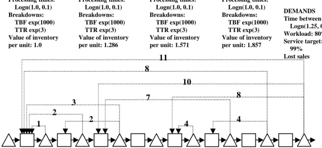
Figure 13 Line configuration #3 and best solution STAGE 1 Processing times: Logn(1.0, 0.1) Breakdowns: TBF exp(1000) TTR exp(3) Value of inventory per unit: 1.0 STAGE 2 Processing times: Logn(1.0, 0.1) Breakdowns: TBF exp(1000) TTR exp(3) Value of inventory per unit: 1.143 STAGE 3 Processing times: Logn(1.0, 0.1) Breakdowns: TBF exp(1000) TTR exp(3) Value of inventory per unit: 1.286 STAGE 4 Processing times: Logn(1.0, 0.1) Breakdowns: TBF exp(1000) TTR exp(3) Value of inventory per unit: 1.428 DEMANDS Time between: Logn(1.25, 0.625) Workload: 80% Service target: 99% Lost sales STAGE 5 Processing times: Logn(1.0, 0.1) Breakdowns: TBF exp(1000) TTR exp(3) Value of inventory per unit: 1.571 STAGE 6 Processing times: Logn(1.0, 0.1) Breakdowns: TBF exp(1000) TTR exp(3) Value of inventory per unit: 1.714 STAGE 7 Processing times: Logn(1.0, 0.1) Breakdowns: TBF exp(1000) TTR exp(3) Value of inventory per unit: 1.857 STAGE 8 Processing times: Logn(1.0, 0.1) Breakdowns: TBF exp(1000) TTR exp(3) Value of inventory per unit: 2.0 2 2 1 4 4 8 3 7 10 8 11
Line configuration #4
Figure 14 shows the ‘best’ control system found by the EA. One would expect the total WIP level in the Conwip system to be closer to 11 units, and local WIP levels to be almost equal at the first stages (as for lines #1 and #2); see table 12. An explanation might be that the demand/capacity ratio is high (0.9) and processing time variability is also high, so demands are frequent and the resource at stage 1 may not be able to keep up the pace at some times because of variability. However, the inventory accumulated at the first stage seems to be redundant because WIP levels at the next two stages are much lower. The generic system solves this problem by adding local control to Conwip: two control loops at the beginning of the line further reduce the release of raw materials. Thus, this is a joint system as defined in section 2.3. The result is a 6% decrease of the total inventory value, at the expense of an increase in complexity (four control loops instead of one).
Table 12 Performance of the best Generic and Conwip systems for line configuration #4
Service WIP allocation Value Target is 95% 1 2 3 4
Best Generic 9.36 95.13% 1.68 1.81 1.91 3.95 Conwip 11 9.95 95.49% 2.50 1.86 1.86 3.82
6.
Discussion
The overall WIP level can change drastically from one production line to another. Indeed, the number of authorization cards in the best Conwip system vary between 4 and 12 for four-stage lines, and between 6 and 27 for eight-stage production lines. Analysis of variance (ANOVA), using table 8 as input (normalized values) and the optimized number of Conwip cards as output, shows that five of the ten factors have an important effect; see table 13:
• Line length (factor A). The longer the line, the more WIP is needed.
Figure 14 Line configuration #4 and best solution
STAGE 1 Processing times: Logn(1.0, 0.5) Breakdowns: TBF exp(1000) TTR exp(3) Value of inventory per unit: 1.0 STAGE 2 Processing times: Logn(1.0, 0.5) Breakdowns: TBF exp(1000) TTR exp(3) Value of inventory per unit: 1.0 STAGE 3 Processing times: Logn(1.0, 0.5) Breakdowns: TBF exp(1000) TTR exp(3) Value of inventory per unit: 1.0 STAGE 4 Processing times: Logn(1.0, 0.5) Breakdowns: TBF exp(1000) TTR exp(3) Value of inventory per unit: 1.0 DEMANDS Time between: Logn(1.11, 0.94) Workload: 90% Service target: 95% Lost sales 3 6 11 10
• Line imbalance (B). More WIP is necessary when the line is balanced; in fact, non-balanced lines have overcapacity, except at the bottleneck, and quick resources require lower inventories.
• Processing time CV (D). The higher the CV, the more WIP is needed.
• Ratio demand rate/capacity (G). The closer the ratio to one, the higher the WIP level.
• Customers' attitude (J). Production lines allowing backorders require a higher WIP level. An explanation is that backordered demands must be fulfilled, so more throughput is required than in the lost sales case.
Efforts to improve the performance of a line should focus on these five important factors, if possible. Surprisingly, factors such as the demand CV (F) and the service level target (H) do not have any effect. The other factors (imbalance pattern, machine reliability, and inventory value ratio) are more important.
Table 13 Regression analysis of the optimal number of Conwip cards as a function of ten factors R2 = 0.956, Adj.R2 = 0.517
Factor A B C D E F G H I J
Regression
coefficient -2.58 3.08 0.92 -2.42 1.08 0.08 2.08 -0.08 -0.75 -2.25
Optimization of the generic model leads to much simpler control systems than we expected. Indeed, whereas the generic model has N(N + 1)/2 loops, the ‘optimized’ solutions have rarely more than N + 1 loops. We also found systems that are neither segmented nor joint, such as line configuration #2 (figure 12). In many cases, however, Conwip is preferred over the ‘optimized’ generic system because the gains in terms of total inventory value are small. Most of these cases have eight stages. More generally, we observe that the benefit of the generic system depends partly on how close to target is the service level in the best Conwip system. Indeed, the largest gains are obtained in configurations for which Conwip has a service level well above target; see lines #2 and #7 in table 14. However, this is not always so: for line #6, Generic reduces inventory by 7.16%, while losing only 0.17% in service (table 14). Thus, significant improvement can be obtained through a more efficient control of WIP along the line, at little expense in terms of service.
There seems to be two main ways of achieving savings in inventory value. First, the release of raw materials can be limited so that the overall inventory level is reduced: the first stage requires authorizations from several other stages, in most cases. Second, when the value of inventory increases along the line, the total inventory value can be reduced by allocating more WIP to early stages (instead of pushing parts to the last stage, as Conwip does): several control loops link the last stage to upstream stages. Obviously these two ways can be combined. In fact, many of the solutions described in the previous section are such combinations; a typical example is line configuration #4 (see figure 14).
Table 14 Performance comparison of Generic versus Conwip for each line configuration
Inventory value Service level Line # Generic Conwip Gain (%) Generic Conwip
(above target) Loss (%) 1 5.99 6.38 6.00 98.91 100.00 (5.00) 1.09 2 4.10 4.73 13.32 96.31 99.21 (4.12) 2.92 3 17.42 17.96 3.00 99.01 99.17 (0.17) 0.16 4 9.36 9.95 5.93 95.13 95.49 (0.49) 0.38 5 11.34 11.70 3.07 99.05 99.31 (0.31) 0.26 6 15.18 16.35 7.16 99.00 99.17 (0.17) 0.17 7 5.30 6.00 11.67 97.48 99.07 (4.07) 1.60 8 7.91 7.99 1.00 99.03 99.12 (0.12) 0.09 9 14.90 15.14 1.58 99.04 99.12 (0.12) 0.08 10 8.52 10.33 9.51 99.00 99.36 (0.36) 0.36 11 41.21 42.36 2.71 95.11 96.00 (1.00) 0.93 12 16.68 17.28 3.47 95.06 96.01 (1.01) 0.99
7. Conclusion
In this paper we proposed a novel approach to the design of pull production control systems for single-product flow lines. Instead of using predefined systems such as Kanban, Conwip, or Base stock, we design customized systems using a generic model that in principle connects each stage of a line with each preceding stage. This generic model integrates not only the three predefined systems, but also their combinations. Moreover, it extends the concept of pull control to systems that have never been investigated in the literature. Optimization of the model shows which potential control loops are actually implemented. To derive general results, we designed twelve production lines, using an experimental design with ten factors (such as line length, demand variability, and machine breakdowns). For each production line we optimized the control system. Despite the complexity of the generic system, results are quite simple most of the time. Simplicity, however, is the main advantage of Conwip, which is preferred for most eight-stage production lines. Nevertheless, customization may yield an inventory value 13% lower than Conwip, while maintaining service on target. Moreover, analysis of our results reveals two important patterns of information flows: one linking each stage to the first stage, and another one linking the last stage to each preceding stage (Integral Control; see section 2.1.iii); these two patterns (possibly simplified: ki; j = ∞) fully characterize many solutions.
The first pattern and the combination of the two patterns have not been mentioned in the literature. Further research is required to investigate the mechanisms involved in these types of control systems.
We see many other extensions of our research. First, it should be possible to extend the concept of customization to other types of production systems, such as assembly/disassembly systems and multi-product flow lines. Second, robustness issues could be considered during the design of customized pull systems. Indeed, a major concern is to design patterns of information flows that are insensitive to variations in the production environment. In Gaury and Kleijnen (1998) we used risk analysis to compare the robustness of four pull systems for a four-stage production line inspired by Toyota. Measuring robustness/risk, however, has a high computational cost, so it is not yet possible to design
customized pull systems using a robustness/risk criterion. Nevertheless, it is possible to compare the robustness of several good solutions.
References
Baker J.E. 1985. Adaptive selection methods for genetic algorithms. Proceedings of the First
International Conference on Genetic Algorithms and Their Applications. J.J. Grefenstette, ed.,
Erlbaum.
Berkley B.J. 1992. A review of the Kanban production control research literature. Production and
Operations Management 1: 393-411.
Berkley B.J. 1996. A simulation study of container size in two-card Kanban systems. International
Journal of Production Research 34(12): 3417-3446.
Bertrand J.W.M. 1983. The use of workload information to control job lateness in controlled and uncontrolled release production systems. Journal of Operations Management 3(2): 79-92.
Bonvik A.M., C. Couch, and S.B. Gershwin. 1997. A comparison of production-line control mechanisms. International Journal of Production Research 35: 789-804.
Bowden R.O., J.D. Hall, and J.M. Usher. 1996. Integration of evolutionary programming and simulation to optimize a pull production system. Computers and Industrial Engineering 31(1-2): 217-220.
Buzacott J.A. 1989. Queueing models of Kanban and MRP controlled manufacturing systems.
Engineering Cost and Production Economics 17: 3-20.
Buzacott J.A. and G.J. Shanthikumar. 1993. Stochastic models of manufacturing systems. Prentice Hall, Englewood Cliffs, New Jersey.
Chang T.-M. and Y. Yih. 1994. Determining the number of kanbans and lotsizes in a generic kanban system: a simulated annealing approach. International journal of production research 32(8): 1991-2004.
Chu C.-H. and W.-L. Shih. 1992. Simulation studies in JIT production. International Journal of
Production Research 30: 2573-2586.
Cochran J.K. and S.-S. Kim. 1998. Optimum junction point location and inventory levels in serial hybrid push/pull production systems. International Journal of Production Research 36(4): 1141-1155.
Dallery Y. and G. Liberopoulos. 1995. A new Kanban type pull control mechanism for multi-stage manufacturing systems. Proceedings of the 3rd European Control Conference 4(2): 3543-3548.
Rome, September 5-8, 1995.
Davis W.J. and S.J. Stubitz. 1987. Configuring a kanban system using discrete optimization of multiple stochastic responses. International Journal of Production Research 25(5): 71-740.
De Jong. 1975. An analysis of the behavior of a class of genetic adaptive systems. Ph.D. Thesis. University of Michigan, Ann Arbor.
De Koster R., and J. Wijngaard. 1989. Local and integral control of workload. International Journal
of Production Research 27(1): 43-52.
De La Maza M. and B. Tidor. 1993. An analysis of selection procedures with particular attention paid to proportional and Boltzmann selection. Proceedings of the Fifth International Conference on
Genetic Algorithms. S. Forrest, ed., Morgan Kaufmann.
Di Mascolo M., Y. Frein, and Y. Dallery. 1996. An analytical method for performance evaluation of Kanban controlled production systems. Operations Research 44(1): 50-64.
Duri C. 1997. Etude comparative des gestions à flux tiré. Thèse de doctorat de l’Institut National
Polytechnique de Grenoble, Laboratoire d’Automatique de Grenoble, Janvier 1997.
Ettl M. and M. Schwehm. 1994. A design methodology for Kanban-controlled production lines using queueing networks and genetic algorithms. Proceedings of the Tenth International Conference on
Systems Engineering. ICSE, 6-8 September, Coventry, UK.
Forrest S. 1985. Scaling fitnesses in the genetic algorithm. In documentation for Prisoners Dilemna and NORMS programs that use the genetic algorithm. Unpublished manuscript.
Gaury E.G.A., J.P.C. Kleijnen, and H. Pierreval. 1997. Configuring a pull production-control strategy through a generic model. CentER Discussion Paper No. 97101. Tilburg University, Netherlands. Gaury, E.G.A., H. Pierreval, and J.P.C. Kleijnen. 1997. Modélisation et simulation dans l’étude de
systèmes de production gérés en Juste-A-Temps. Proceedings of the First French-speaking
AFCET/FRANCOSIM/SCS conference on modeling and simulation 113-123. MOSIM’97, 5-6
June, Rouen, France.
Gaury E.G.A., H. Pierreval, and J.P.C. Kleijnen. 1998. New species of hybrid pull systems. CentER Discussion Paper No. 9831. Tilburg university, Netherlands.
Goldberg D.E. and K. Deb. 1991. A comparative analysis of selection schemes used in genetic algorithms. Foundations of genetic algorithms. G. Rawlins, ed., Morgan Kaufmann.
Goldberg D.E. 1990. A note on Boltzmann tournament selection for genetic algorithms and population-oriented simulated annealing. Complex Systems 4: 445-460.
Goldberg D.E. 1989. Genetic Algorithms in Search Optimization and Machine Learning. Addison-Wesley Publishing Company.
Goldrat E.M. and R.E. Fox. 1986. The race. New York North River Press.
Gstettner S., and H. Kuhn. 1996. Analysis of production control systems: Kanban and Conwip.
International Journal of Production Research 34(11): 3253-3274.
Gupta P.Y. and C.M. Gupta. 1989. A system dynamic model for multi-stage multi-line dual-card JIT-Kanban system. International Journal of Production Research 27: 309-352.
Hillier F.S. and R.W. Boling. 1966. The effect of some design factors on the efficiency of production lines with variable operation times. Industrial Engineering 17: 651-658.
Huang P.Y., L.P. Rees, and B.W. Taylor 1983. A simulation analysis of the Japanese Just-In-Time technique (with Kanbans) for a multiline, multistage production system. Decision Sciences 14: 326-344.
Huang C.-C. and A. Kusiak. 1996. Overview of Kanban systems. International Journal of Computer
Integrated Manufacturing 9: 169-189.
Huang C.-C. and A. Kusiak. 1998. Manufacturing control with a push-pull approach. International
Journal of Production Research 36(1): 251-275.
Hurion R.D.1997. An example of simulation optimization using a neural network metamodel: finding the optimum number of kanbans in a manufacturing system. Journal of the Operations Research
Society 48: 1105-1112.
Kimball G. 1988. General principles of inventory control. Journal of Manufacturing and Operations
Research 1(1): 119-130.
Kimura O. and H. Terada. 1981. Design and analysis of pull systems, a method of multi-stage production control. International Journal of Production Research 19(3): 241-253.
Kleijnen J.P.C. 1987. Statistical tools for simulation practitioners. Marcel Dekker, New York.
Kleijnen J.P.C. 1998. Experimental design for sensitivity analysis, optimization, and validation of simulation models. In Handbook of simulation. Jerry Banks, ed. Wiley, New York.
Krajewski L.J., B.E. King, L.P. Ritzman, and D.S. Wong. 1987. Kanban, MRP, and shaping the manufacturing environment. Management Science 33(1): 39-57.
Liberopoulos G. and Y. Dallery. 1997. A unified framework for pull control mechanisms in multi stage manufacturing systems. Technical report. Laboratoire d'Informatique de Paris 6 (LIP6-CNRS), Université Pierre et Marie Curie, Paris, France.
Lee Y.-J. and P. Zipkin. 1992. Tandem queues with planned inventories. Operations Research 40(5): 936-947.
Meral S. and N. Erkip. 1991. Simulation analysis of a JIT production line. International Journal of
Production Economics 24: 147-156.
Michalewicz Z. 1992. Genetic algorithms + data structures = evolution programs. Springer-Verlag. Michalewicz Z., D. Dasgupta, R. Le Riche, and M. Schoenauer. 1996. Evolutionary algorithms for
constrained engineering problems. Computers and Industrial Engineering 30(4) : 851-870. Mitchell M. 1996. An introduction to genetic algorithms. The MIT press.
Monden Y. 1993. Toyota production system. 2nd edition, Norcross: Institute of Industrial Engineers. Olhager J. and B. Ostlund. 1990. An integrated push-pull manufacturing strategy. European Journal
Paris J.-L. and H. Pierreval. 1997. Configuration of a multiproduct Kanban system using a distributed evolutionary algorithm. Proceedings of the IFAC/IFIP Conference on Management and Control of
Production and Logistics (MCPL’97). Las Campinas, Brazil, 31 Aug. – 3 Sept.
Pegden C. D., R.E. Shannon, and R.P. Sadowski. 1991. Introduction to Simulation using SIMAN / C. McGraw-Hill, New York
Philipoom P.R. and T.D. Fry. 1992. Capacity-based order review/release strategies to improve manufacturing performance. International Journal of Production Research 30(11): 2559-2572. Pierreval H. and L. Tautou. 1997. Using evolutionary algorithms and simulation for the optimization
of manufacturing systems. IIE Transactions 29(3): 181-189.
Powell S.G. and D.F. Pyke. 1998. Buffering unbalanced assembly systems. IIE Transactions 30(1), 55-65.
Price W., M. Gravel, and A.L. Nsakanda. 1994. A review of optimization models of Kanban-based production systems. European Journal of Operational Research 75: 1-12.
Roderick L.M., D.T. Phillips, and G.L. Hogg. 1992. A comparison of order release strategies in production control systems. International Journal of Production Research 30: 611-626.
Roderick L.M., J. Toland, and F. Rodriguez. 1994. A simulation study of Conwip versus MRP at Westinghouse. Computers and Industrial Engineering 26: 137-142.
Sarker B.R. and J.A. Fitzsimmons. 1989. The performance of push and pull systems: a simulation and comparative study. International Journal of Production Research 27(10): 1715-1731.
Sarker B.R. and R.D. Harris. 1988. The effect of imbalance in a Just-In-Time production system: a simulation study. International Journal of Production Research26(1): 1-18.
Savsar M. and A. Al-Jawini. 1995. Simulation analysis of just-in-time production systems.
International Journal of Production Economics 42: 67-78.
Sing N. and J.K. Brar. 1992. Modelling and analysis of Just-In-Time manufacturing systems: A review. International Journal of Operations & Production Management 12: 3-14.
So K.C. and S.C. Pinault. 1988. Allocating buffer storages in a pull system. International Journal of
Production Research 26(12): 1959-1980.
Spearman M.L., D.L. Woodruff, and W.J. Hopp. 1990. Conwip: a pull alternative to Kanban.
International Journal of Production Research 28(5): 879-894.
Sugimori Y., K. Kusunoki, F. Cho, and S. Uchikawa. 1977. Toyota production system and Kanban system materialization of Just-In-Time and Rescpect-For-Human system. International Journal of
Production Research 15(6): 553-564.
Swinehart K.D. and J.H . Blackstone. 1991. Simulating a JIT/Kanban production system using GEMS. Simulation 57(4): 262-269.
Villeda R., R. Dudek, and M.L. Smith. 1988. Increasing the production rate of a just-in-time production system with variable operation times. International Journal of Production Research 26: 1749-1768.
Wang H. and H.-P. Wang. 1990. Determining the number of Kanbans: a step toward non-stock-production. International Journal of Production Research 28(11): 2101-2115.
Yavuz I.H. and A. Satir. 1995. A Kanban-based simulation study of a mixed model just-in-time manufacturing line. International Journal of Production Research 33(4): 1027-1048.
Zipkin P. 1989. A Kanban like production control system: analysis of simple models. Research
Appendix A.
Evolutionary algorithm
Evolution is a method of searching for solutions among a large set of possibilities (search space). Random variations obtained through such operators as mutation and recombination, make species evolve. Natural selection tends to let the fittest individuals survive and reproduce, thus propagating their good genes to the next generations. Evolutionary Algorithms (EAs) reproduce this stochastic process. They begin their search from a set of potential solutions, called a population. Each solution is coded as a chromosome, which has components (also called genes) that are the parameters of the problem to be solved. Generally, the initial population is chosen randomly. EAs make the initial population evolve toward a population that is expected to contain the best solution. For this purpose, EAs use the following reproduction-evaluation cycle: for each iteration – called a generation – solutions from the current population are selected with a given probability, and copies of these solutions are created. This selection is based on the fitness of solutions, relatively to the current population, in the sense that the strongest solutions will have a higher probability of being copied (“survival of the fittest”). In a simulation-optimization approach, a solution is the input value vector of a simulation model; its fitness is a function of the output variables (Pierreval and Tautou, 1997). Part of the copied solutions is submitted to the mutation and recombination operators (which we shall describe later); this process is called reproduction. The recombination mechanism mixes parental information, while passing information on to the descendants or offspring. Mutation introduces innovation into the population. From one generation to another, solutions have higher fitness, globally speaking.
Our goal is to achieve a predetermined service level, while minimizing the total value of inventory (see section 4.3). There are techniques that use EAs for such optimization problems with a constraint (like the service level). The most widely used technique penalizes chromosomes that do not respect the constraint, artificially either decreasing or increasing the fitness of these chromosomes, according to the objective (Michalewicz, 1992). If the objective is to minimize the fitness, then penalizing a solution that does not respect the constraint implies increasing its fitness. Michalewicz, Dasgupta, Le Riche, and Schoenauer (1996) mention the main difficulty is to choose the right level of penalty: if the penalty is too low, the final solution might not respect the constraint; if the penalty is too high, the search might be confined to a small part of the search space and converge to a local optimum.
We evaluate the fitness of individuals through simulation: the EA sends chromosomes as input to the simulation model, which returns a fitness estimation of the corresponding individuals. To estimate the fitness in case of stochastic simulation, we can use either several replications or a single long simulation run.
The main steps of an EA are as follows:
Step 0. Start with the generation counter equal to zero. Step 1. Initialize a population of individuals.
Step 2. Evaluate the fitness of all initial individuals in population. Step 3. Increase the generation counter.
Step 4. Rank the individuals according to their fitness.
Step 5. Copy the individuals in the best half of the population and keep them for the next generation.
Step 6. Select individuals among the cloned ones for children reproduction (selection). Step 7. Recombine selected parents (recombination).
Step 8. Perturb the mated population stochastically (mutation). The new individuals added to the copied ones (step 5) are the new generation.
Step 9. Evaluate the fitness of the new individuals (evaluation).
Step 10. Test the termination criterion (number of generations, fitness, etc.), and stop or return to step 3.
When implementing an EA, five main choices must be made: encoding of solutions, fitness, selection mechanism, evolutionary operators, and parameters of the algorithm. Let us discuss these choices in the case of pull systems. Other studies of pull systems based on EAs and simulation can be found in the literature. Paris and Pierreval (1997) optimize number of Kanbans, container sizes, sequencing rules, and sizes of safety storage for a four-stage production line making three product types. Bowden, Hall, and Usher (1996) determine the number of Kanbans and the order sizes (30 parameters) for an assembly line inspired by a factory of the Whirlpool Corporation.
A.1. Encoding of solutions
In order to identify a pull system, we need to know which stations are linked by control loops, and how many cards each control loop has. In fact, these two types of information may be expressed as follows. When a resource does not need authorizations to produce, it is allowed to produce as long as it has parts in its input inventory. For instance, in a Conwip system all resources except the first one, work according to this principle: they always have the authorization to produce. This can be modeled through a control loop with an infinite number of cards. Thus, a Conwip system is equivalent to a Hybrid system with all Kanban control loops having an infinite number of cards. In this way we build a common representation for all the pull systems represented by the generic model: a chromosome is the list of genes (k1;1, k2;2, k2;1, k3;3, k3;2, …, kN;1) where k1;1, …, kN;1 are the numbers of cards shown in
figure 9 (section 3). We are interested in genes with a domain of the type D ∪ {∞}, where D is a finite
A.2. Fitness
We minimize the objective function f inspired by Michalewicz et al. (1996), which we define as follows:
if service ≥ target, f = inventory value,
if service < target, f = inventory value/(service/k)p
where p is the penalty parameter and k is a scaling factor chosen such that service/k <1. Thus, when a solution does not respect the service constraint, the objective function is increased by a penalty factor equal to (service/k)p. When the service constraint is respected, the optimum is the solution with the lowest total inventory value.
A.3. Selection
One of the most popular selection systems is the roulette wheel (Goldberg, 1989). In that system the decision whether to select a chromosome is made according to a probability assigned to each chromosome. That probability is based on the fitness of the chromosome, such that the one with the best fitness has a higher chance of surviving. The literature provides many alternatives to the roulette-wheel principle:
•sigma-scaling also accounts for the standard deviation of the individual fitness (Forrest, 1985);
•elitism preserves a number of the best individuals, from one generation to another (De Jong, 1975);
•Boltzmann selection uses the principle of crystallization that is also used in simulated annealing
(Goldberg, 1990, De la Maza and Tidor, 1993);
•rank selection maintains the pressure of selection, even when the fitness of individuals gets very
close to each other (Baker, 1985);
•tournament selection makes individuals compete against each other (Goldberg and Deb, 1991).
We choose to implement the elitism and the roulette wheel principles. A part of the new population is an exact copy of the best solutions in the previous generation (elitism), whereas another part is selected randomly from the previous population (roulette wheel) and is changed by evolutionary operators.
A.4. Evolutionary operators
The combination of EA and simulation is rather time-consuming. In order to save computer time, uninteresting solutions should be avoided. The understanding of card-based control systems can help identifying such solutions. Local control affects the performance of the production system only if there is no stronger constraint at a higher level (it is a necessary not a sufficient condition). In other words, a control loop should have a smaller number of cards than any control loop above it. In a Hybrid system, for instance, each Kanban number should be smaller than the number of Conwip cards. Otherwise, the corresponding control loop does not have any effect on the performance of the