Approximating Tree Edit Distance through String Edit Distance

Title Approximating Tree Edit Distance through String Edit_Distance

Author(s) Akutsu, Tatsuya; Fukagawa, Daiji; Takasu, Atsuhiro

Citation Algorithmica (2010), 57(2): 325-348

Issue Date 2010-06

URL http://hdl.handle.net/2433/113886

Right The original publication is available at www.springerlink.com

Type Journal Article

Approximating Tree Edit Distance through String

Edit Distance

∗

Tatsuya Akutsu

Bioinformatics Center, Institute for Chemical Research, Kyoto University,

Uji, Kyoto 611-0011, Japan.

e-mail: [email protected]

Daiji Fukagawa

Atsuhiro Takasu

National Institute of Informatics,

Chiyoda-ku, Tokyo 101-8430, Japan.

e-mail:

{

daiji,takasu

}

@nii.ac.jp

Abstract

We present an algorithm to approximate edit distance between two ordered and rooted trees of bounded degree. In this algorithm, each input tree is transformed into a string by computing the Euler string, where labels of some edges in the input trees are modified so that structures of small subtrees are reflected to the labels. We show that the edit distance between trees is at least 1/6 and at most O(n3/4) of the edit distance between the transformed strings, wheren is the maximum size of two input trees and we assume unit cost edit operations for both trees and strings. The algorithm works in O(n2) time since computation of edit distance and reconstruc-tion of tree mapping from string alignment takesO(n2) time though transformation itself can be done inO(n) time.

Key Words. tree edit distance, string matching, approximation algorithms, em-bedding, Euler string

∗_{A preliminary version of this paper appeared in the Proceedings of the 17th Annual International}

Symposium on Algorithms and Computation(ISAAC’06), Lecture Notes in Computer Science, 4288, pp. 90-99, 2006. This work is partially supported by Grants-in-Aid on Scientific Research on Priority Areas “Cyber Infrastructure for the Information-explosion Era” and “Systems Genomics”, and Grant-in-Aid #16300092 from MEXT, Japan.

1

Introduction

Recently, comparison of tree-structured data is becoming important in several diverse ar-eas such as computational biology, XML databases and image analysis [4, 12, 20]. Though various measures have been proposed for comparison of trees [4], theedit distancebetween rooted and ordered trees is well-studied and widely-used [14, 18, 19, 21]. This tree edit distance is a generalization of the edit distance for two strings [2, 17], which is also well-studied and widely-used for measuring the similarity between two strings. In this paper, we use tree edit distance and string edit distance to denote the distance between rooted and ordered trees and the distance between strings, respectively.

It is well-known that the string edit distance can be computed in O(n2) time by a simple dynamic programming algorithm, wherenis the maximum length of input strings. Recently, extensive studies have been done on efficient (quasi linear time) approximation and low distortion embedding of string edit distances [2, 3, 13, 15, 17].

For the tree edit distance problem, Tai [18] first developed a polynomial time algo-rithm, from which several improvements followed [5, 9, 14, 21]. Among these, a recent algorithm by Demaine et al. [9] is the fastest in the worst case and works in O(n3) time where n is the maximum size of input trees. They also proved an Ω(n3) lower bound for the class of decomposition strategy algorithms. Therefore, it is quite difficult to develop ano(n3) time exact algorithm for the tree edit distance problem.

Garofalakis and Kumar developed an algorithm for efficient embedding of rooted and ordered trees [10]. Their algorithm provides an approximate tree edit distance with a guaranteed O(log2log∗n) factor in O(nlog∗n) time, where log∗n denotes the number of log applications required to reduce n to 1 or less. However, the distance considered there is not the same as the tree edit distance: move operations are allowed in their distance. Several practical algorithms have been developed for efficient computation of lower bounds of tree edit distances [12, 20], but these algorithms do not guarantee upper bounds of tree edit distances. Therefore, it is required to develop algorithms for efficient approximation and/or low distortion embedding for trees in terms of the original definition of the tree edit distance. It should be noted that for the case of strings, an efficient approxima-tion/embedding algorithm was first proposed for edit distance with block copies, block uncopies and block moves [7, 16], which was soon modified to take care of string edit

distance with block moves only [6], and then extensive studies followed for edit distance without moves [2, 3, 13, 15, 17].

In order to approximate the tree edit distance, we studied a relation between the tree edit distance and the sting edit distance for the Euler strings [1]. It was shown that the tree edit distance is at least half and at most 2h+ 1 of the edit distance for the Euler strings, wherehis the minimum height of two trees. This result gives good approximation if the heights of input trees are low. However, it does not guarantee any upper bounds of tree edit distances if the heights of input trees are O(n). In this paper, we improve this result by modifying the Euler string. Modification is done by changing labels of some edges in the trees so that structures of small subtrees are reflected to the labels. Though the modification is slight, a novel idea is introduced and much more involved analysis is performed. We show that the unit cost edit distance between trees is at least 1/6 and at most O(n3/4) of the unit cost edit distance between the modified Euler strings, where we assume that the maximum degree of trees is bounded by a constant. This result leads to the first O(n3−) time algorithm for computing the unit cost tree edit distance with a guaranteed approximation ratio (for bounded degree trees). Though this result is not practical, it would stimulate further developments. It should be noted that the current best approximation ratio within near linear time algorithms for string edit distance is aroundO(n1/3) [3] even though extensive studies have been done in recent years. Though we consider theunit cost edit distances in this paper, the result can be extended as in [1] for more general distances for which the ratio of the maximum cost of an edit operation to the minimum cost of an edit operation is bounded by a constant for both strings and trees.

2

String Edit Distance and Tree Edit Distance

Here we briefly review the string edit distance and the tree edit distance. We consider strings over a finite or infinite alphabet Σ_S. For string s and integer i, s[i] denotes the

ith character of s, s[i . . . j] denotes s[i]. . . s[j], and |s| denotes the length of s. We may use s[i] to denote both the character itself and the position. An edit operation on a string s is either a deletion, an insertion, or a substitution of a character of s. The edit distance between two strings s₁ and s₂ is defined as the minimum number of operations

to transform s₁ intos₂, where only unit cost operations are considered in this paper. We use ED_S(s₁, s₂) to denote the edit distance between s₁ and s₂.

We also define an alignment between two strings. An alignment between two strings

s₁ and s₂ is obtained by insertinggap symbols (denoted by ‘-’ where ‘-’ ∈/ Σ_S) into or at either end of s₁ and s₂ such that the resulting strings s₁ and s₂ are of the same length l, where it is not allowed for each i= 1, . . . , lthat both s₁[i] and s₂[i] are gap symbols. The

costof alignment is given bycost(s₁, s₂) =l_i=1f(s₁[i], s₂[i]),wheref(x, y) = 0 ifx=y= ‘-’, otherwisef(x, y) = 1. Then, an optimal alignment is an alignment with the minimum cost. It is straight-forward to see that the cost of an optimal alignment is equal to the edit distance. For example, consider strings s₁ =“TCGTGCAT” and s₂=“CGATCCT”. Then, the following is an optimal alignment.

T C G - T G C A T - C G A T C C - T

(a) (b) (c) (d)

In this case, (a) and (d) correspond to deletions, (b) corresponds to an insertion, and (c) corresponds to a substitution. Thus, we have ED_S(s₁, s₂) = 4.

Next, we define edit distance between trees (for the details, see [4]), where we only consider the unit cost case. Let T be a rooted ordered tree, where “ordered” means that a left-to-right order among siblings is given in T. Moreover, we assume that each node v

has a label label(v) from a finite alphabet Σ_T. |T|denotes the size (the number of nodes) of T. An edit operation on a tree T is either a deletion, an insertion, or a substitution (see also Fig. 1):

Deletion: Delete a non-root nodev inT with parentu, making the children ofv become the children of u. The children are inserted in the place of v as a subsequence in the left-to-right order of the children of u.

Insertion: Complement of delete. Insert a node v as a child of u in T making v the parent of a consecutive subsequence of the children of v.

A B A B _C B D D B A A B A B B D D B A deletion of ’C’ insertion of ’C’ T1 T2

(A)

(B)

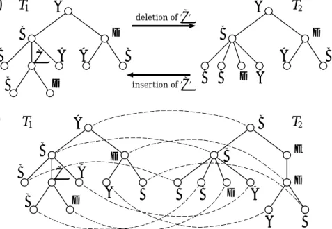
Figure 1: (A) Insertion and deletion operations. (B) T₂ is obtained by deletion of a node with label ‘C’, insertion of a node with label ‘E’ and substitution for the root node. A mapping corresponding to this edit sequence is also shown by dashed curves.

The edit distance between two trees T₁ and T₂ is defined as the minimum number of operations to transform T₁ into T₂. We use ED_T(T₁, T₂) to denote the edit distance between T₁ and T₂.

It is known that there exists a close relationship between the edit distance and the

ordered edit distance mapping (or just a mapping) [4]. M ⊆ V(T₁)×V(T₂) is called a mapping if the following conditions are satisfied for any pair (v₁, w₁), (v₂, w₂) ∈ M: (i)

v₁ =v₂ iff. w₁ =w₂, (ii)v₁ is an ancestor ofv₂iff. w₁is an ancestor ofw₂, (iii)v₁ is to the left of v₂ iff. w₁ is to the left of w₂. Let ID(M) be the number of pairs having identical labels in M. It is well-known that the mapping M maximizing ID(M) corresponds to the edit distance, for which ED_T(T₁, T₂) =|T₁|+|T₂| − |M| −ID(M) holds.

3

Euler String

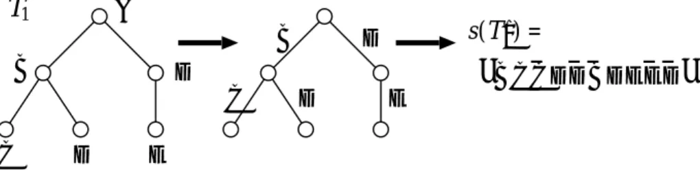
Our transformation from a tree to a string is based on the Euler string [14], which is obtained by traversing a tree using the Euler tour. In this section, we review the Euler string and our previous result on the Euler string [1].

A

T

Figure 2: Construction of an Euler string.

For simplicity, we treat each treeT as an edge labeled tree: the label of each non-root node v in the original tree is assigned to the edge {u, v} where u is the parent of v. It should be noted that information on the label on the root is lost in this case. But, it is not a problem because the roots are not deleted or inserted. In what follows, we assume that the roots of two input trees have identical labels (otherwise, we just need to add 1 to the distance).

The depth-first search traversal of T (i.e., visiting children of each node according to their left-to-right order) defines an Euler tour of a tree T. That is, the depth-fist search gives an Euler path beginning from the root and ending at the root where each edge

{w, v} is traversed twice in the opposite directions. We use EE(T) to denote the set of directed edges in the Euler tour of T. Let Σ_S = {a, a|a ∈ Σ_T}, where a /∈ Σ_T. Let (e₁, e₂, . . . , e_2n−2) be the sequence of directed edges in the Euler path of a tree T with n

nodes. From this, we create the Euler string s(T) of length 2n−2. Let e={u, v} be an edge in T, where u is the parent of v. Suppose that e_i = (u, v) and e_j = (v, u) (clearly,

i < j). We define i₁(e) and i₂(e) by i₁(e) = i and i₂(e) = j, respectively. That is, i₁(e) and i₂(e) denote the first and second positions of e in the Euler tour, respectively. Then, we define s(T) by letting s(T)[i₁(e)] = L(e) and s(T)[i₂(e)] = L(e), where L(e) is the label ofe (see also Fig. 3).

Proposition 1 [1, 19] s(T₁) =s(T₂) if and only if ED_T(T₁, T₂) = 0. Moreover, we can reconstruct T from s(T) in linear time.

T

T

B

D

A

C

B

D

A

C

B

D

A

C

D

B

C

A

D

B

C

A

D

B

C

A

D

Figure 3: Example for the case of ED_T(T₁, T₂) = Θ(h)·ED_S(s(T₁), s(T₂)) [1].

Proof. We associate each edit operation on T₁ with two edit operations on s(T₁). For a deletion ofe(i.e., deletion of the deeper node of the endpoints ofe), we associate deletions of L(e) and L(e). For an insertion of e, we associate insertions of L(e) and L(e). For a substitution of e to e, we associate substitutions of L(e) and L(e) to L(e) and L(e), respectively. Clearly, the resulting sequence transforms s(T₁) to s(T₂) and the cost is

2·ED_T(T₁, T₂). 2

Lemma 2 [1] ED_T(T₁, T₂) ≤ (2h+ 1) ·ED_S(s(T₁), s(T₂)), where h is the minimum height of two input trees.

It was shown in [1] that this bound is tight up to a constant factor. Fig. 3 gives an example such thatED_S(s(T₁), s(T₂)) = 4 and ED_T(T₁, T₂) = Θ(h).

4

Modified Euler String

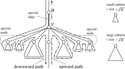
As shown in the above, the approximation ratio of the tree edit distance through the edit distance between the Euler strings is not good if the minimum height of input trees is high. In order to improve the worst case approximation ratio, we modify labels of some edges in the input trees so that structures of small subtrees are reflected to the labels. For example, we consider trees shown in Fig. 3. Suppose that label “AC” is assigned

special node

v

u

downward path

upward path

small subtree

n

_n

Figure 4: Special nodes, special edges, and large subtrees.

to each edge just above each node having children with labels ‘A’ and ‘C’. Similarly, suppose that labels “BD”, “AD” and “BC” are assigned to appropriate edges. Then,

ED_S(s(T₁), s(T₂)) = Θ(h) should hold. But, changes of labels should be performed carefully in order to keep distance distortion not too large.

Before explaining changes of labels, we need several definitions (see also Fig. 4). Let

size(v) be the size (the number of nodes) of the subtree induced byv and its descendants. A subtree rooted at v is called large if size(v) > α, where α is a parameter defined as

α = n1/2. Otherwise, it is called small. We call w_i a special node if size(w_i) ≤ α and

size(v)> α wherev is the parent of w_i. Then, we have the following proposition, where

depth(v) denotes the depth of v (i.e., the length of the path from the root tov).

Proposition 2 For each node v in T, there exists at most one special node in the path from the root to v. Moreover, if v is a leaf and depth(v) ≥ α, there exists exactly one special node in the path.

Proof. Let (v₀ =r, v₁, v₂,· · ·, v_k =v) be the path from the root to v. Since size(v₀) > size(v₁) > size(v₂) > · · · > size(v_k) holds, at most one v_i can satisfy size(v_i−1) > α ≥ size(v_i).

Ifv is a leaf and depth(v)≥α, there must existv_i satisfyingsize(v_i−1)> α≥size(v_i)

For a nodev in T₁ orT₂, id(v) is an integer such thatid(v) =id(v) if and only if the subtree induced by v and its descendants is isomorphic (including labels) to the subtree induced byv and its descendants. Since we only consider subtrees induced by some node

v in T₁ or T₂ and its descendants and we assume that Σ_T is a finite alphabet (i.e., |Σ_T| is a constant), all id(v)’s can be computed in O(n) time [11], where n= max{|T₁|,|T₂|}. Furthermore, each id(v) can be an integer between 1 and 2n and thus can be stored in a word (i.e., O(logn) bits). In the following, we briefly review the algorithm for computing

id(v). For details, refer to [11].

We construct a suffix tree T for a string s(T₁)·“$”·s(T₂)· “#”, where ‘$’ and ‘#’ are letters not appearing in Σ_S, and x·y denotes the concatenation of x and y. Then, each suffix staring from a letter in Σ_T corresponds to a subtree in T₁ or T₂. For each leaf l

in T corresponding to such a suffix, let sz(l) be the size of the corresponding subtree in

T₁ orT₂. Let a(l) be the first nodev, encountered along the path from the root of T to the leaf l, such that the length of the substring corresponding to the path from the root to a(l) is no less than 2·sz(l). Then, it is shown in [11] that the subtrees corresponding to l₁, l₂, . . . , l_k are isomorphic to each other if and only if a(l₁) = a(l₂) = · · · = a(l_k). Thus, by identifying all a(l)’s, we can partition all subtrees into the equivalent classes. Identification of alla(l)’s can be done by using the depth first search traversal ofT. When the first leaf l corresponding to a subtree is found, we find the nodea(l) by coming back fromlto the root ofT. Next, we visit all descendants ofa(l) and put leaves corresponding to subtrees inT₁ andT₂into the same class. Then, we deletea(l) and all of its descendants and resume the depth first search traversal. It is shown in [11] that this algorithm works in O(n) time for a finite alphabet, including the construction of a suffix tree. After the set of equivalent classes is obtained, we can assign different integers to different classes in

O(n) time. Therefore, we can assign id(v) to all nodes in O(n) time.

Using id(v), we define edge labels, with which the modified Euler strings are con-structed. Let v be a node in T₁. Let u be the parent of v and w₁, . . . , w_k be the children of v (Similarly, we define v, u, and w₁, . . . for T₂). If at least one of w_i’s is special,

{u, v} is called a special edge. Otherwise, {u, v} is not special and the original label (i.e., label in Σ_T) of v is assigned to {u, v}. For a special edge {u, v}, let w_i1, . . . , w_ih

id(v, w_i1, . . . , w_ih) = id(v, w_i1, . . . , w_il ) if and only if h = l, label(v) = label(v), and

id(w_ij) = id(w_ij) holds for all j = 1, . . . , h. Then, we assign id(v, w_i1, . . . , w_ih) to {u, v}

where we assume w.l.o.g. (without loss of generality) that id(. . .) ∈/ Σ_T. It should be noted that ifv has at least one special children, information of the subtrees of the special children is reflected to the label of {u, v}.

These indices can be computed in O(n) time as follows. We simply sort all tuples (i.e., all (label(v), id(w_i1), . . . , id(w_ih))’s) in lexicographic order. Since we assume that the maximum degree is bounded, each tuple is a sequence of at most constant number of integers between 1 and 2n+|Σ_T|. Furthermore, each label of a special edge does not depend on labels of other special edges. Therefore, we can obtain the sorted list of tuples in O(n) time by performing radix sort only once.

Using the above labeling of edges, we create a modified Euler string ss(T) as in s(T). It should be noted that ss(T) and s(T) differ only on labels of special edges. It is also worthy to note thatss(T₁) andss(T₂) can be constructed inO(n) time fromT₁ andT₂. In what follows, we consider editing operations onT₁ andT₂, by which the number of nodes in trees may change. However, α is fixed to α = n1/2 = (max{|T₁|,|T₂|})1/2 throughout editing operations.

Proposition 3 Substitution, insertion or deletion of a node in T₁ or T₂ affects the label of at most two special edges.

Proof. Since there exists at most one special node in the path from the root to each node

v (though there may exist many special edges), each edit operation can change the label of at most one existing special edge, including the case where a special edge becomes non-special. In addition, at most one non-special edge in the path may become special. Therefore, each edit operation affects the label of at most two special edges. 2

5

Analysis

In this section, we show the following main theorem using several propositions and lemmas, where we assume that the maximum degree of input trees are bounded by a constant. In what follows, we may identify a directed edge (u, v), a node v and the corresponding letter in ss(T) if there is no confusion.

Theorem 1 _O(n1_3/4) ·ED_T(T₁, T₂) ≤ ED_S(ss(T₁), ss(T₂)) ≤ 6·ED_T(T₁, T₂).

5.1

Upper Bound of String Edit Distance

First, we prove the latter half of Theorem 1, which is easily done as in Lemma 1.

Lemma 3 ED_S(ss(T₁), ss(T₂)) ≤ 6·ED_T(T₁, T₂).

Proof. As in the proof of Lemma 1, we associate each edit operation on T₁ with two edit operations onss(T₁). But, in this case, additional substitutions are required because labels of some edges may change. From Proposition 3, it is seen that labels of at most two edges change per edit operation, which correspond to substitutions of 4 letters in ss(T₁).

2

It is to be noted that both Lemma 3 and Proposition 3 hold for anyα ≥1. Therefore, the above lemma holds even when ED_T(T₁, T₂) isO(n). In order to prove the former half of Theorem 1, it is enough to consider the case where |T₁| and |T₂| are Θ(n). Otherwise

||T₁| − |T₂|| > cn would hold for some constant c and thus the former half obviously holds since ED_S(ss(T₁), ss(T₂))> cn holds. Therefore, we can assume w.l.o.g. that α is Θ(|T₁|1/2) = Θ(|T₂|1/2).

5.2

Construction of Tree Mapping from String Alignment

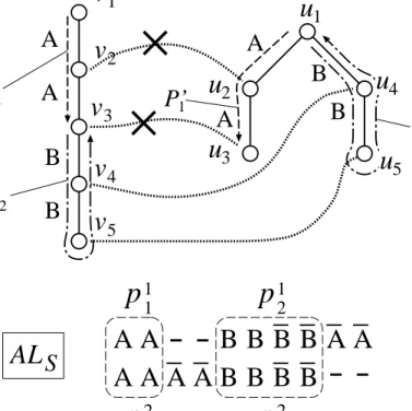
In order to prove the rest half inequality, we show a procedure for obtaining a mapping between T₁ and T₂ from an (not necessarily optimal) alignmentAL_S between ss(T₁) and

ss(T₂) with cost d. Before showing details of the procedure, we describe an outline. We first create a mapping M₁ that is induced by corresponding downward paths, where downward (and upward) paths are to be defined later. Next, we modifyM₁ toM₂ so that labeling information on special edges is reflected (i.e., mapping pairs for right subtrees rooted at special children are added to M₁). However, such mappings (both M₁ andM₂) may contain pairs violating ancestor-descendant relations. Thus, we delete inconsistent pairs from M₂ (the resulting mapping is denoted as M₃). Finally, we add large subtrees included in upward paths, then delete some inconsistent pairs fromM₃, and get the desired mapping M₄.

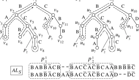
B A B C B A C C A B v₂ v1 v3 v4 v5 v6 v7 v8 v₉ v10 v₁₁ B A B C B A C C A D u₂ u1 u3 u4 u5 u8 u9 u₁₀ u11 u₁₂ A u6 u7 B A B B A C B B A C C A C B C A A B B A B B A C B A A B A C C A C B C A A D AL_S v₁₂ B D C B B B C

T

T

p

p

p

p

Figure 5: Construction of M₁ from AL_S. Regions surrounded by dashed lines in

AL_S correspond to maximal substring pairs. The path corresponding to p1₂ (resp.

p2₂) is divided into P₂ and P₃ (resp. P₂ and P₃), where P₂ and P₂, and P₃

and P₃ are twins respectively. The path corresponding to p1₁ (resp. p2₁) is di-vided into P₁ (resp. P₁) and an empty path. P₁, P₁, P₃ and P₃ are down-ward paths, whereas P₂ and P₂ are upward paths. P₁ contains central edges of (v₁, v₂),(v₂, v₅),(v₅, v₆), and P₂ contains central edges of (v₆, v₅),(v₅, v₂),(v₂, v₁). M₁ =

{(v₂, u₂),(v₃, u₃),(v₄, u₄),(v₅, u₅),(v₆, u₆),(v₉, u₁₀),(v₁₀, u₁₁)}.

5.2.1 Construction of M₁

In this first phase, we create a mapping M₁ from AL_S. M₁ acts as a backbone for the whole mapping. In order to explain the construction of M₁, we define downward paths and related terms.

An edge (u, v) is called a downward edgeif v is a child of u. Otherwise, (u, v) is called anupward edge. For each downward edge e, edenotes the upward edge corresponding to

e(i.e., e= (v, u) ife= (u, v)). For each edgee= (u, v), we let src(e) =u anddst(e) =v. Let {(p1₁, p2₁),(p1₂, p2₂), . . .} be the set of maximal substring pairs (p1_i from ss(T₁) and

p2_i fromss(T₂)), each of which corresponds to a maximal consecutive region (with length at least 2) in AL_S without insertions, deletions or substitutions. Note that p1_i and p2_i

correspond to isomorphic paths in T₁ and T₂. We divide each path corresponding to pj_i

one path may be empty. Let p1_i[k] be the first letter corresponding to a downward edge (u, v) such that a letter corresponding to (v, u) does not appear inp1_i. Then, (p1_i[1. . . k−

1], p2_i[1. . . k−1]) and (p1_i[k . . .], p2_i[k . . .]) are the upward segment pair and the downward segment pair, respectively. Two paths P inT₁ and P in T₂ corresponding to an upward segment pair are called upward paths, and P (resp. P) is called a twin of P (resp.

P). Two paths corresponding to a downward segment pair are called downward paths, and twins are defined in the same way as above. A subtree that is fully included in a downward (resp. upward) path is called aleft subtree(resp. right subtree). An edge (u, v) in a downward (resp. upward) path is called acentral edgeif (v, u) does not appear in the same path. Thus, central edges are the edges (in downward paths and upward paths) not appearing in any left or right subtrees. For a downward path (resp. an upward path)P, a

downward central path (resp. upward central path) denotes the path consisting of central edges in P and height(P) denotes the number of edges in this central path. It is possible that there is no central edge in an upward path (i.e., height(P) = 0), where a downward path must contain at least one central edge from the definition. In such a case, the path consists of a large or small subtree. In the following, such a subtree is regarded as a left subtree and the path corresponding to the subtree is regarded as a downward path. It is to be noted that the roots of such subtrees are not included M₁ since these roots are not destinations of downward edges (see alsoP₂ and P₂ in Fig. 9).

Suppose that ss(T₁)[i] corresponds to ss(T₂)[i] in any downward segment pair by means ofAL_S, and downward edges (u, v) and (u, v) correspond toss(T₁)[i] andss(T₂)[i], respectively. Then, we letM₁ be the set of such (v, v)’s defined as above (see Fig. 5 for an example). If there exist pairs of twin downward paths consisting of only subtrees, pairs of the roots of the corresponding subtrees are added to M₁.

It should be noted that in our previous work [1], we construct a mapping between T₁

and T₂ from all corresponding pairs of left and right subtrees, which is shown to be a valid mapping. From that result, it is seen that mapping pairs in M₁ corresponding to left subtrees are consistent with each other. Thus, the inconsistency will be caused by central edges and (small and large) right subtrees that are to be added in constructions of

M₂ andM₄. The following proposition implies that we only need to take care of nodes in downward edges, left subtrees and right subtrees since the order of approximation ratio

T

u

v

T

u’

v’

w

w’

M

M

- M

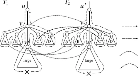
Figure 6: Addition of mapping pairs toM₂. In this case, mapping pairs betweenC andC, and between D and D are added toM₂. Each cross means that there exist insertion(s), deletion(s) or substitution(s) around the point.

does not change if we ignore the other O(d) nodes.

Proposition 4 The number of nodes not appearing in destinations (i.e.,dst(e)) of down-ward central edges, left or right subtrees is O(d).

Proof. Since there are O(d) insertions, deletions and substitutions, the number of edges not appearing in downward paths or upward paths is O(d). The nodes not on these edges

must be on downward central edges or in left or right subtrees. 2

5.2.2 Construction of M₂

M₁ gives a mapping for left subtrees and central edges, but does not give a mapping for right subtrees. In the construction of M₂, mapping pairs for small right subtrees are added, whereas mapping pairs for large right subtrees are added in the construction of

M₄.

Let e = (u, v) and e = (u, v) be a pair of corresponding central special edges in M₁

(i.e., (v, v) ∈ M₁). Suppose that there exists a node w in T₁ satisfying the following conditions (see Fig. 6):

(i) (u, v) and (v, w) belong to the same downward path, (v, u) and (w, v) belong to the same upward path,

(ii) the subtree rooted at wis large.

Then, there must exist a node w inT₂ satisfying analogous conditions because (u, v) and (u, v) are special edges having the same label. It is to be noted that from condition (i), there must exist insertion(s), deletion(s) or substitution(s) in the large subtree rooted at

w. We add mapping pairs to M₁ that are induced by the small right subtrees rooted at the special children of v and v, where the correspondence between right subtrees in

T₁ and T₂ are given by id’s of the special children. Since we assume that the maximum degree is bounded, detection of corresponding special children can be done in a constant time per special edge. We let the resulting mapping be M₂.

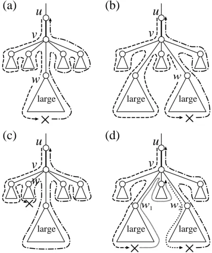
Some examples explaining the above conditions are given in Fig. 7. In case (a) and case (b), mapping pairs are added. In case (c), mapping pairs are not added becausew is a root of a small subtree. In case (d), mapping pairs are not added because (w₁, v) and (v, u) belong to different upward paths and (u, v) and (v, w₂) belong to different downward paths. As shown below, the number of central edges such as in (c) and (d) is not so large.

Proposition 5 The number of central edges which do not satisfy the condition in the construction of M₂ is O(d).

Proof. We prove the proposition for central edges in T₁. The proposition can be proven for central edges in T₂ in an analogous way and thus the total number should still be

O(d).

First, we consider the case that condition (i) is violated for a central edge (u, v) (see also Fig. 7 (d)). Then, v must have at least two subtrees in each of which there exist insertion(s), deletion(s) or substitution(s). Since the total number of insertions, deletions and substitutions is O(d), we can have O(d) central edges that do not satisfy condition (i) (recall that a tree such that every internal node has at least two children can have at most 2l−1 nodes where l is the number of leaves).

Next, we consider condition (ii). For a central edge (u, v) that violates condition (ii), we associate the small (left or right) subtree rooted at a special child of v in which there exist insertion(s), deletion(s) or substitution(s) (see also Fig. 7 (c)). This small subtree can be associated with at most one central edge. Since the total number of insertions, deletions and substitutions is O(d), we can have O(d) central edges that do not satisfy

(a)

(b)

(c)

u

v

w

u

v

w

u

v

w

u

v

(d)

w

w

Figure 7: Examples for explaining the conditions used in the construction ofM₂. Mapping pairs for right subtrees are added to M₂ in case (a) and case (b), whereas these are not added in case (c) or case (d).

5.2.3 Construction of M₃

In the construction of M₃, we delete inconsistent pairs. Since M₁ is constructed from downward paths obtained from string alignment, which preserve left-right relationships, andM₂is constructed from central special edges, left-right relationships between mapping pairs are preserved. Thus, we focus on violation of ancestor-descendant relationships.

Let (v, v) ∈ M₁ be a pair of the highest nodes in a pair of twin downward paths, where the highest node in any downward path is determined uniquely. Let ˆP_v (resp. ˆP_v)

be the set of nodes in the path from the root to v (resp. v). We delete any (u, u)∈M₁

T

u

v

r

T

u’

v’

r’

p

_p’

q

_q’

M

Figure 8: Deletion of inconsistent mapings fromM₂ in the construction ofM₃. Bold lines correspond to ˆP_v and ˆP_v.

small right subtrees rooted at children of u and u (see Fig. 8). In this paper, deletion of a subtree(resp. a region or a node) means that all mapping pairs containing nodes in the subtree are deleted from the current mapping set, but does not mean that the subtree is deleted from the tree. Addition of a subtree is defined analogously. We execute this deletion procedure for all downward segment pairs in an arbitrary order, where we allow that the same mapping pairs are deleted multiple times. Then, the resulting mappingM₃

is determined uniquely. M₃ is a valid mapping as shown below.

Proposition 6 M₃ is a valid mapping between T₁ and T₂.

Proof. Since mapping pairs between small right subtrees are obtained from central special edges, these are consistent with other mapping pairs if the corresponding central special edges are consistent. Therefore, in the following, we focus on inconsistency caused byM₁. Mapping pairs created by a single pair of twin downward paths are consistent with each other since twin downward paths are isomorphic. Therefore, inconsistency is caused by (u, u)∈M₁ and (w, w)∈M₁ belonging to different pairs of twin downward paths.

Suppose that u is an ancestor of w but u is not an ancestor of w. Then, u must be an ancestor of the node v which corresponds to the highest node of the downward path containingw, butucannot be an ancestor of the nodev which corresponds to the highest

T

T

u

u

u

P’

P’

A

A

B

B

v

A

P

A

B

B

v

v

v

P

A A

B B

A A

B

AL

_S

A A

B

B

B

B

B

A A

p

p

p

p

u

u

v

Figure 9: An example of construction of M₃. P₁ and P₁ are downward paths ob-tained from (p1₁, p2₁), and P₂ and P₂ are downward paths obtained from (p1₂, p2₂). M₁ =

M₂ = {(v₂, u₂),(v₃, u₃),(v₄, u₄),(v₅, u₅)} is shown by bold dotted lines, from which

M₃ ={(v₄, u₄),(v₅, u₅)} is obtained by deleting (v₂, u₂),(v₃, u₃).

node of the downward path containing w (see also Fig. 8). Therefore, it is enough to examine consistency between all pairs (u, u) in M₁ and all pairs (v, v) of highest nodes in twin downward paths. Since the other cases can be proven in an analogous way, the

proposition holds. 2

It should be noted that left subtrees are never deleted since any node in a left subtree cannot be an ancestor of nodes not in the subtree. Mapping pairs between left subtrees will be consistent with other pairs in M₃ (and inM₄).

Fig. 9 gives an example of construction of M₃. In this case, (v₂, u₂) is deleted from

M₂ since v₂ ∈ Pˆ_v4 but u₂ ∈/ Pˆ_u4. Similarly, (v₃, u₃) is deleted from M₂. The readers may think that too many mapping pairs are deleted if the paths corresponding to AA are much longer than the paths corresponding to BB. However, in such a case, AL_S should

have many unaligned A’s and thus d should have been so large thatd·O(n4/3) =O(n) is satisfied (recall that the tree edit distance is always O(n)). This intuition is to be proven concretely in Lemma 10.

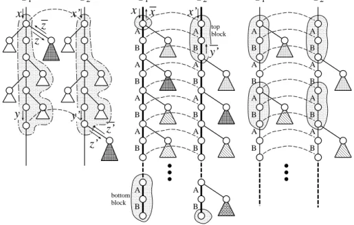
5.2.4 Construction of M₄

Finally, we add all large subtrees (i.e., subtrees with more thann1/2 nodes) that are fully included in upward paths, and then delete inconsistent mapping pairs.

In the following, we assume that the number of large subtrees attached to a node is at most one. If multiple large subtrees are attached to a node, we can regard these large subtrees as one large subtree. In this final phase, we consider the following two cases (see Fig. 10):

(A) the number of edges in an upward path is at most 2d,

(B) the number of edges in an upward path is greater than 2d, where we assume w.l.o.g. that all the central edges of an upward path are shared by the central edges in a downward path (otherwise, we can cut the upward path into multiple upward paths without affecting the order of the approximation ratio since the total number of upward paths remains O(d)).

As to be shown later, there is some periodicity in case (B), which plays an important role in both construction and analysis of M₄. In all cases, mapping pairs between large right subtrees, which are induced by twin upward paths, are added to M₄. None of these added pairs is deleted. Instead, mapping pairs between some nodes in central paths and small right subtrees are deleted. Therefore, we only describe deletion procedures in the following.

For case (A), we only show the procedure for the case where only one large subtree is included in an upward path (see Fig. 11). This procedure is referred as the cleanup procedure. Extension to the other cases is straight-forward since it is enough to repeat the same procedure. Letz . . . z(resp. z. . . z) be the sequence of directed edges corresponding to the large subtree of T₁ (resp. T₂). Let x = (u, v) ∈ EE(T₁) be a parent of z, and let

y = (u, v) ∈ EE(T₂) be a parent of z (recall that EE(T) denotes the set of directed edges in the Euler tour of T). Let x and y correspond to x and y in downward paths,

A B A B A B A B x x A B A B A B A B top block x’ y’

(A)

(B-1)

T

T

T

T

(B-2)

T

T

Figure 10: Construction of M₄. Gray triangles denote large subtrees, and thin dashed lines denote (parts of) M₃. (A) Gray regions are deleted. (B-1) Gray regions and central edges (shown by bold lines) are deleted, and mappings between small right subtrees are modified. (B-2) For each pair of large right subtrees, gray regions are deleted as in case (A). Different from case (A), the size of each deleted region isO(dn1/4).

respectively. We assume w.l.o.g. thaty is a descendant of x. Then, we delete v and ith ancestors of v for i = 1,2, . . . , d along with attached small right subtrees (see Fig. 11). Though the cleanup procedure is very simple, analysis is a bit involved. In the following, we show the correctness of the procedure.

For two strings s₁ and s₂, s₁·s₂ denotes the concatenation of s₁ and s₂. For a string

s, #₀(s) and #₁(s) denote the number of letters corresponding to downward edges and upward edges, respectively. Let Δ(s) = #₁(s)−#₀(s).

Proposition 7 ED_S(s₁, s₂)≥ |Δ(s₁)−Δ(s₂)|.

Lemma 4 Let s₂ = s1₂·s2₂. Suppose that Δ(s1₂) = h >0 holds, and Δ(s1₁)≤ 0 holds for any prefix s1₁ of s₁. Then, ED_S(s₁, s₂)≥h holds.

Proof. From the definition of string edit distance,

T

x

y

T

y’

x’

M

z

z

z’

z’

u’

v’

u

v

T

x

y

T

y’

x’

M

Figure 11: Details of case (A) in M₄. In this case, mapping pairs between large checked triangles are added and mapping pairs between nodes in central edges and small right subtrees are deleted.

where the minimum is taken over all partitions s₁ = s1₁·s2₁ of s₁. Since ED_S(s1₁, s1₂) ≥h

holds for any partition s₁ =s1₁·s2₁ from the assumption and Proposition 7, we have

ED_S(s₁, s₂) ≥ h+ED_S(s2₁, s2₂) ≥ h.

2

Lemma 5 Suppose that only a pair of identical large subtrees is added in the construction of M₄ and the cleanup operation is performed. Then, the resulting mapping is valid. Proof. It is to be noted that mapping pairs corresponding to left subtrees and large right subtree are consistent with each other [1]. Thus, inconsistency is caused only when ancestors of v (resp. v) (along with attached small right subtrees) are mapped to non-ancestors of v (resp. v). In this proof, we consider mapping pairs only for ancestors of

v. Mapping pairs for ancestors of v can be treated in an analogous way. We need to consider two cases (see also Fig. 12): (A-1) ancestors of v are mapped to descendants of

v, (A-2) ancestors of v are mapped to non-descendants of v.

First we consider the case of (A-1). Let pand q be the (d+ 1)th and dth ancestors of

T

x

T

z

z’

z’

z

y’

s

s

T

x

T

z

z

s

s

z’

z’

(A-1)

(A-2)

x’

Figure 12: Illustration of the proof of Lemma 5.

a child q of v inM₃. Modification of the proof for the other cases (e.g., p is mapped to a descendant of v) is straight-forward.

Lets₁be a substring ofss(T₁) starting from (p, q) and ending just beforez. Lets₂ be a substring ofss(T₂) starting from (v, q) and ending just beforez. Then, Δ(s₁) =−(d+1) and Δ(s₂) = 0 hold. Since (p, q) and z correspond to (v, q) and z respectively in AL_S, we have from Proposition 7:

d ≥ ED_S(s₁, s₂) ≥ | −(d+ 1)−0|=d+ 1.

This is a contradiction. Thus,pcannot be mapped tov (or its descendant). Since at most

d ancestors of v can be mapped to v or its descendants, the cleanup operation removes the inconsistency in the case of (A-1).

Next we consider the case of (A-2). In this case, we assume w.l.o.g. that v is mapped to w which is not an ancestor or descendant of v, or v. Let x be the incoming edge to

w. Let p be the (d+ 1)th ancestor of v. Suppose thatp is mapped to a node p which is an ancestor w but is not an ancestor of v. Modification of the proof for the other cases is straight-forward.

Let q be the parent of p. Let s₁ be a substring of ss(T₁) starting just after x and ending just before z. Let s₂ be a substring ofss(T₂) starting just afterx and ending just

beforez. Let s1₂ be the prefix ofs₂ ending at (p, q). Then, Δ(s1₁)≤0 holds for all prefix

s1₁ of s₁, and Δ(s1₂)≥ d+ 1 holds. Since x and z correspond to x and z respectively in

AL_S, we have from Lemma 4:

d ≥ ED_S(s₁, s₂) ≥ d+ 1.

This is a contradiction. Thus, p cannot be mapped to a non-ancestor of v. Therefore, the cleanup operation removes the inconsistency also in the case of (A-2). 2 Before considering case (B), we need the following proposition (see also Fig. 10 (B-1)), which can be shown by counting the numbers of downward edges and upward edges in

AL_S, where depth(e) denotes the depth of v for a downward edge e = (u, v) (resp. an upward edgee = (v, u)).

Proposition 8 Suppose that a downward edge x ∈ EE(T₁) corresponds to a downward edge x ∈EE(T₂)in AL_S. Then, |depth(x)−depth(x)| ≤d holds. Furthermore, suppose that x corresponds to an upward edge y ∈EE(T₂) in AL_S. Then,

|depth(x)−depth(y)| ≤ d

holds.

For case (B), central paths should haveperiodicitybecause upward central paths match with identical downward central paths at different positions. From Proposition 8, we can see that the length of a period is at mostd. That is, central paths are repetitions of a chain of length at most d. Suppose that x and x correspond to x and y in AL_S, respectively (see also Fig. 10). We assume w.l.o.g. that the downward paths begin with x and x in

T₁ and T₂ respectively, and y is a descendant of x. Then, the subtree consisting of the nodes in the central path between dst(x) and dst(y) and the nodes in their small right subtrees is called a block. A subtree isomorphic to the block is also called a block. It can be seen that blocks appear repeatedly in the vertical direction in both T₁ and T₂. We consider the following two cases:

(B-1) the size of a block is greater thanβ, where β=dn1/4.

M

M

T

x

T

x’

T

x

T

x’

Figure 13: Details of case (B1) in M₄, where the upper half part is only shown in this figure. Bold dotted lines denote mappings, and gray triangles denote large right subtrees. Gray regions and central edges are deleted. Furthermore, mappings between small right subtrees are modified.

the height of each block is at most d, the height of an upward path is at most n, and

β· #(central edges in the upward path)

d ≤ n

holds from the definition of the block. We delete the top block fromT₂, the bottom block from T₁, the central edges in the current downward paths from T₁ and T₂, small right subtrees attached to the top node in the top block of T₁ and small right subtrees attached to the bottom node in the bottom block of T₂ (see Fig. 13). Furthermore, we modify the mapping between the remaining small right subtrees so that mapping pairs between small right subtrees are consistent with those between large right subtrees. In other wards, mapping pairs between left subtrees are induced by the twin downward paths, whereas mapping pairs between right subtrees are induced by the twin upward paths. It is to be noted that in Fig. 13, the left subtree attached to the top ‘A’ in T₁ is mapped to the left subtree attached to the top ‘A’ in T₂, whereas the small right subtree attached to the top ‘A’ in T₁ is mapped to the small right subtree attached to the second top ‘A’ in T₂. However, there is no inconsistency because central edges are deleted.

(B-2) the size of a block is at mostβ.

In this case, for each pair of corresponding large right subtrees, we perform the cleanup procedure as in case (A). However, different from case (A),O(β) =O(dn1/4) nodes are deleted per pair since the nodes in at most two consecutive blocks are deleted per large right subtree.

As in the case of (A), we can see that the resulting mapping is valid. Therefore, we have:

Proposition 9 M₄ is a valid mapping between T₁ and T₂.

5.3

Analysis of Lower Bound of String Edit Distance

Now we analyze the lower bound of ED_S(ss(T₁), ss(T₂)). We estimate the cost (i.e., the number of corresponding edit operations) of M₄, assuming that the cost of AL_S is

d = ED_S(ss(T₁), ss(T₂)). For that purpose, we estimate the number of mapping pairs deleted or ignored in the construction. For two edgesx= (u, u) andy= (v, v),dist(x, y) denotes the length of the shortest path betweenuandv. For two nodesuandv,dist(u, v) denotes the length of the shortest path between u and v.

It is straight-forward to see the following propositions (see also Proposition 4).

Proposition 10 The number of nodes not appearing in any downward or upward path is O(d).

Proposition 11 The number of downward (resp. upward) paths is O(d).

Proposition 12 The total number of nodes in downward paths that do not appear inM₁ is O(d).

Due to the above propositions, we only need to consider hereafter upward paths and deleted mapping pairs.

d+1

x

d+1

x

_x’

v

T

T

x’

Figure 14: Explanation of Lemma 7. y should be located in the gray region.

Lemma 6 The number of nodes in the small subtrees in the upward paths that are not included in M₂ is O(dn1/2).

Proof. It is seen from Proposition 5 that the number of central special edges that are not taken into account forM₂ isO(d). Since we assume that the maximum degree is bounded by a constant, the number of nodes in the small right subtrees rooted at special children of a special edge is O(n1/2). There may exist small subtrees that are fully included in the upward paths but are not attached to special edges. But, the total size of such small

subtrees per upward path isO(n1/2). 2

Next, we estimate the number of deleted mapping pairs in constructing M₃. For that purpose, we show using some lemmas that not so many nodes are deleted from central edges of each downward path.

Lemma 7 Suppose that a downward edge x ∈ EE(T₁) corresponds to a downward edge x ∈ EE(T₂) in AL_S. Suppose also that an upward edge x ∈ EE(T₁) corresponds to an upward edge y ∈EE(T₂). Then, dist(x, y)≤3d+ 3.

Proof. From Proposition 8, |depth(x)−depth(y)| ≤ d holds. Let v be the ancestor of

src(x) such that dist(v, src(x)) = d+ 1 (If there does not exist such a node, we let v

be the root). From the above fact, it is seen that y is in the subtree rooted at v and

depth(y)−depth(v)≤2d+ 2 holds (see Fig. 14). Since dist(v, src(x))≤d+ 1 holds, we

Lemma 8 Let x ∈ EE(T₁) and y ∈ EE(T₁) be downward edges belonging to the same downward central path where x is an ancestor of y. Suppose that x and y belong to the same upward central path. Let x, y, z and w in EE(T₂) correspond in AL_S to x, y, y and x, respectively. Moreover, suppose that depth(y)−depth(x) > 100d. Then, at most

20d nodes are deleted from the downward central (sub)path beginning from x and ending at y in the construction of M₃.

Proof. From Lemma 7, we see that the central upward path from z to w must have an overlap with the central downward path from x to y with the amount of at least

dist(x, y)−20d nodes (see Fig. 15).

Let v be the lowest common ancestor of y and z. Let v be the node inT₁ such that (v, v) ∈ M₂, which also means (v, v) ∈ M₁ since these nodes belong to central edges. Let (u, u) ∈ M₁ be a pair of beginning nodes of twin downward paths such that u is a descendant of dst(y). Then, u must be a descendant of v because u is in the part of Euler path beginning from y and ending at z. Therefore, (u, u) cannot delete any node in the consecutive part of a downward central path beginning from dst(x) and ending at

v.

Since w and z belong to the same upward central path, bothsrc(w) anddst(w) are ancestors of dst(z). Thus, we consider two cases: (i) dst(w) is a descendant of dst(x), (ii) dsp(w) is a ancestor ofdst(x) or w coincides with x. We lett =src(w) in case of (i), otherwise we lett =dst(x). Lettbe the node inT₁ such that (t, t)∈M₁. Then, any downward path in T₁ (resp. T₂) begins either from a descendant of dst(y) (resp. v) or from a non-descendant ofdst(x) (resp. t). In the former case, any central edge betweent

and v (resp. betweent and v) cannot be deleted as explained before. In the latter case, neither t or t is an ancestor of the beginning node of a downward path. Therefore, any node in the central edges between t and v (resp. between t and v) cannot be deleted.

Since the number of nodes between tandv (resp. t andv) is at leastdist(x, y)−20d,

the lemma holds. 2

It should be noted that 100d and −20d are determined with large margin since we discuss in this paper the order of the approximation ratio.

Next, we bound the number of nodes appearing in M₁ which may be deleted in the construction ofM₃. LetP = (v_i1, v_i2, . . . , v_ik) be a consecutive part of a downward central

T

x

x

T

y

_y

x’

y’

z’

w’

v’

>

dist(x,y)-20d

t’

t

v

Figure 15: Explanation of Lemma 8.

path in T₁. Let P = (u_i1, u_i2, . . . , u_ik) be the corresponding part of a downward central path in T₂. P (resp. P) is called a maximal central subpath if (P, P) is maximal (i.e., cannot be extended) under the condition that (v_ik, v_ik−1, . . . , v_i1) is a consecutive part of an upward central path of T₁ and (u_ik, u_ik−1, . . . , u_i1) is a consecutive part of an upward central path ofT₂. Furthermore,P (resp. P) is called amaximal conserved central subpath

ifP (resp. P) is a maximal central subpath and (v_ik, v_ik−1, . . . , v_i1) and (u_ik, u_ik−1, . . . , u_i1) are in twin upward central paths. It is to be noted that (v_ih, v_ih−1) and (u_ih, u_ih−1) do not necessarily correspond to each other in AL_S. See Fig. 16 for an example.

Lemma 9 The number of nodes that appear in central downward paths but do not belong to maximal conserved central subpaths of length greater than 100d is O(d2).

Proof. Since there are O(d) downward paths and O(d) upward paths, the number of maximal central subpaths is O(d). The number of edges in central downward paths but not in maximal central subpaths is also O(d).

The number of nodes in maximal central subpaths whose length is at most 100d is

O(d)×O(d) = O(d2). The number of nodes in maximal central paths but not in maximal conserved central subpaths isO(d)×O(d) =O(d2) because the total number of downward central subpaths for which corresponding upward central paths are not twins isO(d) and the length of such a subpath is O(d).