Traffic Forecasting in Smart Cities
Final Master Thesis
Juan Jos´
e V´
azquez Gim´
enez
Advisor Mari Paz Linares Herreros - inLab FIB Co-advisor Jamie Arjona Mart´ınez - inLab FIB
Tutor Josep Casanovas Garcia
Tutor department Department of Statistics and Operations Research (DEIO) Master Master in Innovation and Research in Informatics
Specialty Data Science Date 15 de gener de 2019
Abstract
Nowadays, cities must address the challenge of sustainable mobility. Traffic state forecasting plays a key role in mitigating traffic congestion in urban areas. For example, predicting path travel time is a crucial issue in navigation and route planning applications. Furthermore, the increasing penetration of Information and Communication Technologies makes Floating Car Data become an important source of real-time data for Intelligent Transportation Systems applications.
In the context of an educational cooperation agreement with the research group of the inLab FIB focused on smart mobility, this master thesis deals with the problem of urban traffic forecasting when Floating Car Data is available. The main goal is to perform traffic forecasting with machine learning methods and evaluate this kind of solutions under different conditions: size of the network, penetration rate of the floating cars, prediction horizon and the amount of required data.
The current state of the art shows that most of the newly proposed methods for urban traffic fore-casting use a Deep Learning approach. A comparison of four neural network approaches (recurrent and convolutional) is presented to evaluate the capabilities of Deep Learning methods to solve the problem.
Different tests are proposed in order to evaluate the developed Deep Learning models, and also to analyze how the different proposed factors affect the forecasting accuracy. The performed experiments are designed through a microscopic traffic simulation approach to emulate Floating Car Data.
The main conclusions from the obtained results show that the methods without a convolutional com-ponent present the best performance for all the tested experimental scenarios.
Acknowledgements
Ahora que estoy en el final de este camino echo la vista atr´as y me doy cuenta de la cantidad de gente que ha aportado su granito de arena a este proyecto. Personas que en mayor o menor medida me han ayudado a llegar hasta aqu´ı, a veces (incluso) sin saberlo. Me gustar´ıa agradecer a todos aquellos que, aunque sus nombres no aparezcan entre estas l´ıneas, han sido muy importantes para mi durante esta etapa. Dicho esto, considero que existen ciertas personas sin las cuales no habr´ıa sido posible y a los que quiero mencionar de forma especial.
En primer lugar, a Mari Paz por depositar su confianza en mi. Desde que surgi´o la idea por primera vez, hasta la realizaci´on de esta, ha luchado a m´ı lado por este proyecto, incluso m´as de lo que requiere su papel de directora. En todo momento he contado con su apoyo, tanto a nivel profesional como personal, ayud´andome siempre que lo he necesitado. Tambi´en a Jamie, porque es un privilegio contar con un co-director como ´el. El hecho de que este proyecto tenga un enfoque similar a su tesis, aun tratando temas diferentes, le convierte en alguien idoneo con el que compartir problemas, dudas y retos comunes. Adem´as, su admirable pasi´on por formarse as´ı como su inquietud por aprender algo nuevo cada d´ıa le hacen el compa˜nero de aventura perfecto. Es una suerte que personas como ellos sean mis directores, pero sobretodo mis amigos.
A Josep, por sus consejos, por darme la oportunidad de pertenecer a inLab y por hacer posible este proyecto. Me parece una labor excepcional la que se hace desde el laboratorio, ayudando a los estudiantes a formarse a trav´es de su participaci´on en proyectos reales y apostando por la transferencia de conocimiento desde la universidad.
Al incre´ıble equipo del inLab, tanto estudiantes como personal, por convertir el entorno de trabajo en un lugar a donde te apetece ir cada ma˜nana. En especial a Marta, por cuidar de todos y no tirar nunca la toalla. A Gonzalo, Albert, Pau, Sergio y Tote por intentar entender lo que escribo y ayudarme a expresarlo mejor. Y a Juan y Josefran, por cierta tarde de horas interminables viendo como la temperatura de la GPU sub´ıa y bajaba.
Y por ´ultimo, y no por ello menos importante, a mi familia y amigos por preocuparse de mi en los peores momentos y ofrecerme una v´alvula de escape cuando m´as lo necesito. En especial a Sara, que ha sufrido en primera persona todos los altibajos de este proyecto con una paciencia inagotable, sac´andome siempre una sonrisa. ¡No podemos formar mejor equipo!
Contents
1 Introduction 1
1.1 Context . . . 1
1.2 The traffic forecasting problem . . . 2
1.3 Objectives and motivations . . . 5
1.4 Temporal planning . . . 6
1.5 Master thesis outline . . . 9
2 State of the art 11 2.1 k-Nearest Neighbors . . . 12
2.2 Neural Networks . . . 14
2.2.1 Deep Learning . . . 15
2.3 Hybrid Methods . . . 16
2.4 Other Methods . . . 17
2.5 Summary and Conclusions . . . 19
3 Neural Networks required background 23 3.1 Neural Networks preliminary concepts . . . 23
3.2 Recurrent Neural Networks . . . 26
3.2.1 Long Short-Term Memory Neural Networks . . . 26
3.3 Convolutional Neural Networks . . . 30
3.3.1 Convolution operation . . . 30
3.3.3 Convolutional Neural Network structure . . . 32
3.4 Neural Network parameters . . . 32
4 Development 37 4.1 Proposed models . . . 37
4.1.1 Long Short-Term Memory and Gated Recurrent Unit Neural Networks . . . 37
4.1.2 Spatiotemporal Recurrent Convolutional Networks . . . 39
4.1.3 High-Order Graph Convolutional Long Short-Term Memory Neural Network . . . 42
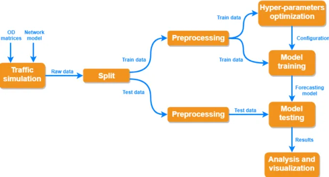
4.2 Implementation . . . 44
4.2.1 Traffic simulation . . . 45
4.2.2 Split and preprocessing . . . 46
4.2.3 Hyper-parameters optimization and model training . . . 47
4.2.4 Model testing, results analysis and visualization . . . 47
5 Computational experiments 49 5.1 Simulated data . . . 49 5.1.1 Traffic demand . . . 50 5.1.2 Traffic networks . . . 52 5.2 Error measures . . . 53 5.3 Hyper-parameters optimization . . . 54
5.3.1 Hyper-parameter optimization algorithm . . . 54
5.3.2 Hyper-parameter optimization configuration . . . 55
5.3.3 Optimized hyper-parameters . . . 56
5.4 Experiments . . . 58
5.4.1 FCD penetration rate . . . 59
5.4.2 Prediction horizon . . . 66
5.4.3 Amount of training data . . . 77
6 Final comments and conclusions 85 6.1 Conclusions . . . 85
6.2 Contributions . . . 87
List of Figures
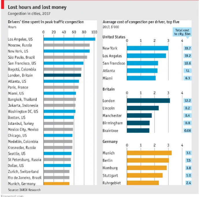
1.1 Results of the article named The hidden cost of congestion published in 2018. Source:
https://www.economist.com/ . . . 3
1.2 Gantt diagram of the main project tasks planning. . . 8
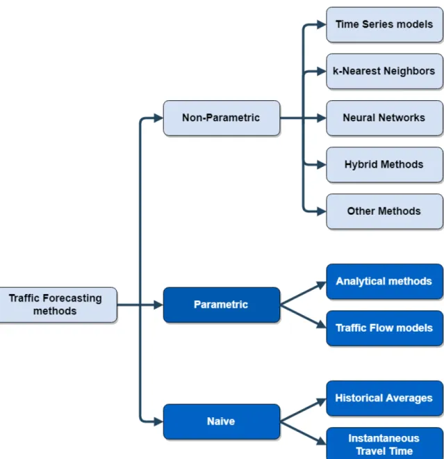
2.1 Traffic forecasting methods classification. The clear boxes denotes the studied thoroughly methods. . . 13
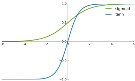
3.1 A graphical representation of the sigmoid function and the hyperbolic tangent (tanh) func-tion. Source: http://ronny.rest/blog/ . . . 24
3.2 Basic schema of a simple Neuron. Source: https://torres.ai/ . . . 25
3.3 Basic schema of a simple Neural Network. Source: http://mindwise-groningen.nl/ deep-learning-the-beautiful-mind/ . . . 25 3.4 Schema of an unrolled Recurrent Neural Network. Source: http://colah.github.io/ . . 26
3.5 Schema of a Long Short Term Memory network layer. Source: http://colah.github.io/ 27
3.6 Notation of the LSTM schemas. Source: http://colah.github.io/ . . . 27
3.7 The focus of the LSTM schema for the first step. Source: http://colah.github.io/ . . 27
3.8 The focus of the LSTM schema for the second step. Source: http://colah.github.io/ . 28
3.9 The focus of the LSTM schema for the third step. Source: http://colah.github.io/ . . 28
3.10 The focus of the LSTM schema for the fourth step. Source: http://colah.github.io/ . 29
3.11 GRU schema. Source: http://colah.github.io/ . . . 30
3.12 Schema of a convolutional operation. Source: https://towardsdatascience.com/@torres. ai . . . 31
3.13 Schema of the output of a convolutional layer. Source: https://towardsdatascience. com/@torres.ai . . . 31
3.14 Schema of the convolutional and pooling operations application.
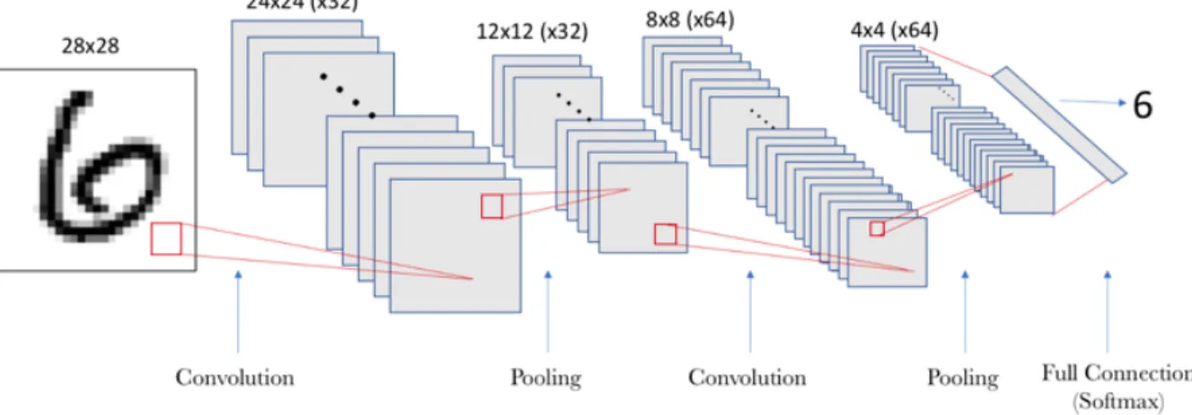
3.15 Schema of a Convolutional Neural Network model that identifies the number represented
in a image. Source: https://towardsdatascience.com/@torres.ai . . . 33
4.1 Simple example of the transformation between the FCD input and the S corresponding dataset. . . 38
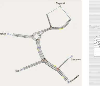
4.2 Image of the Camp Nou simulation model. . . 40
4.3 Representation of the Camp Nou simulation model printed with ’X’ and ’ ’. . . 40
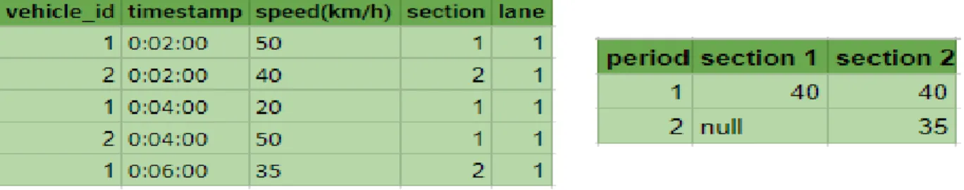
4.4 Conceptual example of the inputsItgeneration. Source: Yu et al. [2017] . . . . 41
4.5 Examples of the input images for the SRCN model. . . 41
4.6 Schema of the SRCN model structure. . . 42
4.7 Graphical example ofAe1 andAe2 matrices. Source: Cui et al. [2018] . . . 43
4.8 Graphical simple example of aF F Rmatrix. Source: Cui et al. [2018] . . . 43
4.9 Simplified schema of the data flow between the different developed parts of the project. . 44
5.1 Distribution of the number of daily trips (in thousands) in a working day. Source: https: //www.atm.cat/web/en/observatori/mobility-surveys.php . . . 51
5.2 Distribution of trips in function of the transportation mode in a working day. Source: https://www.atm.cat/web/en/observatori/mobility-surveys.php . . . 51
5.3 Left, the map of the real simulated zone in the Camp Nou model Source: https://www. google.com/maps/. Right, the Camp Nou simulation model schema. . . 52
5.4 Left, the map of the real simulated zone in the Amara modelSource: https://www.google. com/maps/. Right, the Amara simulation model schema. . . 53
5.5 Plots of the MAE (left) and RMSE (right) errors of the models in function of the penetration rate in the Camp Nou network. . . 62
5.6 Plots of the training computational time of the models in function of the penetration rate in the Camp Nou network. . . 62
5.7 Plots of the number of missing values in function of the penetration rate in the Camp Nou network. . . 63
5.8 Plots of the MAE (left) and RMSE (right) errors of the models in function of the penetration rate in the Amara network. . . 64
5.9 Plots of the training computational time of the models in function of the penetration rate in the Amara network. . . 65
5.10 Plots of the number of missing values in function of the penetration rate in the Amara network. . . 66
5.11 Plots of the number of empty sections in function of the penetration rate in the Amara network. . . 67
5.12 Plots of the MAE (left) and RMSE (right) errors of the models in function of the short-term prediction horizon in the Camp Nou network. . . 70
5.13 Plots of the training computational time of the models in function of the short-term pre-diction horizon in the Camp Nou network. . . 71
5.14 Plots of the MAE (left) and RMSE (right) errors of the models in function of the long-term prediction horizon in the Camp Nou network. . . 72
5.15 Plots of the training computational time of the models in function of the long-term predic-tion horizon in the Camp Nou network. . . 73
5.16 Plots of the MAE (left) and RMSE (right) errors of the models in function of the short-term prediction horizon in the Amara network. . . 74
5.17 Plots of the training computational time of the models in function of the short-term pre-diction horizon in the Amara network. . . 75
5.18 Plots of the MAE (left) and RMSE (right) errors of the models in function of the long-term prediction horizon in the Amara network. . . 76
5.19 Plots of the training computational time of the models in function of the long-term predic-tion horizon in the Amara network. . . 76
5.20 Plots of the MAE (left) and RMSE (right) errors of the models in function of the amount of training data in the Camp Nou network. . . 80
5.21 Plots of the training computational time of the models in function of the amount of training data in the Camp Nou network. . . 80
5.22 Plots of the MAE (left) and RMSE (right) errors of the models in function of the amount of training data in the Amara network. . . 81
5.23 Plots of the training computational time of the models in function of the amount of training data in the Amara network. . . 82
5.24 Plot of the average speed of all the network sections of the Camp Nou scenario during 7 days of data. . . 83
List of Tables
5.1 Set of the proposed experiments for the penetration rate. . . 60
5.2 Results of the penetration rate experiments in the Camp Nou network. . . 61
5.3 Results of the penetration rate experiments in the Amara network. . . 64
5.4 Set of the proposed experiments for the short-term prediction horizons. . . 68
5.5 Set of the proposed experiments for the long-term prediction horizons. . . 69
5.6 Shift value in function of the prediction horizon. . . 69
5.7 Results of the short-term prediction horizon experiments in the Camp Nou network. . . . 70
5.8 Results of the long-term prediction horizon experiments in the Camp Nou network. . . 71
5.9 Results of the short-term prediction horizon experiments in the Amara network. . . 73
5.10 Results of the long-term prediction horizon experiments in the Amara network. . . 74
5.11 Set of the proposed experiments for the amount of training data. . . 78
5.12 Results of the amount of training data experiments in the Camp Nou network. . . 79
Chapter 1
Introduction
This initial Chapter introduces the context of the proposed master thesis carried out for the inLab FIB1, the innovation and research laboratory of the Faculty of Informatics at Universitat Polit`ecnica
de Catalunya. In addition, the traffic forecasting problem is presented, including a description of its key issues. Furthermore, main objectives and motivations of the project are exposed, together with some research questions. In addition, the temporal planning of the whole project is described. Finally, an outline of the whole document is presented in order to expose the applied methodology and organize its content.
1.1
Context
According to the data published by the European Comision in 20172, urban areas are the “engine” of
economic growth and employment, as around 85% of the European Union’s gross domestic product is generated in cities. Therefore, the population is more and more concentrated in the cities. In 2010, 73% of European citizens lived in urban areas and this percentage is expected to increase to over 80% by 2050. Due to the population concentration growth, cities face multiple problems related to, or caused by, transport and traffic. One of the most important problems is the private vehicle use increment and with it, the urban networks saturation.
Urban traffic saturation is a problem in multiple ways. Figure 1.1 shows the result of the article named The hidden cost of congestion3published byThe Economist publication in 2018. On the left is shows the hours drivers spent of some cities in peak traffic congestion during 2017. Time wasting implies a money wasting too, the economic cost per driver are quantified in the right figure (in thousands of dollars). Also, the economic costs (in billions of dollars) that it means for the cities of United States, United Kingdom,
1https://inlab.fib.upc.edu/
2https://ec.europa.eu/transport/themes/urban/urban_mobility_en 3
and Germany. But urban traffic has not only time and economic effects according to theWorld Health Organization the exposure to ambient (outdoor) air pollution causes 4.2 million deaths every year. The same organization classifies the fuel combustion from motor vehicles (e.g. cars and heavy-duty vehicles) as one of the major human activities sources of outdoor air pollution. Accidents on the roads and noise pollution are also bad consequences of the traffic, especially in urban areas.
All these problems can be relieved through the decrease of road traffic congestion, especially in urban cores. Lana et al. [2018] classify the different strategies of mitigation of traffic congestion in three: increasing and improving infrastructures, proposing new transport alternatives and managing traffic flows. Due to the difficulties presented by the first one (limited by topographical, budgetary and social factors) and the dependency of the second one to political decisions, the improvement of the traffic management is the main followed strategy. In the last years, the development of new technological solutions, the computational capability of systems and the quantity of data generated have been incremented. These factors favor the development and the use of new Traffic Management Systems (TMS) and Traveler Information Systems (TIS). Some of the key features for this kind of systems need traffic forecasting, for example to anticipate actions for future situations or to perform navigation and route planning taking into account the future traffic state. The following Section describes the traffic forecasting problem and what aspects are used to differentiate between its subproblems.
1.2
The traffic forecasting problem
The traffic forecasting problem is very extensive and it includes some subproblems according to different issues. One of the most important features in the traffic forecasting problem is the kind of network where the predictions are performed. Usually, they are classified in urban networks and freeways. The topology is very different because urban networks contain more and shorter links while freeway networks are composed of few but larger links. Also, some authors include the arterial network category when the prediction is performed only over the main sections of an urban network. Typically, forecasting in urban areas is more difficult because the behavior of the drivers inside the network is less predictable.
Another key feature in this problem is the prediction horizon. The literature uses the expressions short-term and long-term to classify them. Although it is not clear exactly what horizons each group refers to, the short-term name is used for predictions from 1 minute to around 30 minutes or 1 hour depending on the author. For larger prediction horizons, the long-term name is used. Of course, despite this binary classification, the prediction horizon can variate between 1 minute to hours or days. In general, the complexity of the problem increases and the forecasting accuracy decreases with larger horizons.
Besides the kind of network and the horizon time, the traffic prediction problem is determined by what variable and with which granularity is predicted. Traffic forecasting can be performed for different variables, the most presents in the literature are four:
Figure 1.1: Results of the article namedThe hidden cost of congestion published in 2018. Source:
time (measured in vehicles/second or vehicles/hour).
• Traffic density: it is the number of vehicles located in a determined area at the same time (measured in vehicles/meter or vehicles/kilometer).
• Average speed: it is the average speed for the vehicles in a site (measured in kilometer/hour or meter/second).
• Travel time: it is the time that takes a vehicle to travel from a origin point to its destination (measured in seconds, minutes or hours).
These predicted variables can be used in different scales, like a specific point in a network, a section (a link or a part of a link) of the network and the whole network (or a sector for the network).
Also, as seen on most of the machine learning problems, the prediction performed can be regression or classification. This depends on if the prediction is performed over a continuous number (the presented predicted variables) or over a finite set of values (a discretization of the previously predicted variables). So, depending on the final goal, the traffic forecasting solution could try to advance the average speed of each section, the general traffic state of a network (for example free, medium or congestion), the number of vehicles that will pass through some point, etc.
Finally, the last issue to be considered is the data source used. Nowadays, traffic data is generated in multiple ways and many types of systems can be used to it. Following, the most usual traffic data sources are listed:
• User surveys: Traditionally, most of the other options did not exist and the traffic was measured through surveys performed directly over the population. This data source has been replaced by other automatic ways (mentioned below) which are cheaper and collect better data.
• Sensors: These devices are able to register some traffic features like the presence of a vehicle, its speed, etc. In the last years and following with the smart cities evolution, the presence of traffic sensors has grown and they have been improved. For example, one of the first used sensors was the loop detector which is able to detect vehicles in a specific position. This kind of devices requires roadworks for their installation, thus their relocation is too expensive. Currently, other modern options like the ANPR (Automatic Number-Plate Recorder) are used, with an easier installation and the capability to identify which cars pass through a point. Despite these improvements, they are only able to register the activity in a fixed location and the quantity of them needed to cover a whole city is very high.
• Cameras: Although the main goal of traffic cameras is to offer a real-time monitorization of the network state, in recent years they have been used as traffic data collectors. It is a very good way to reuse installed systems, but the use of camera records as traffic data needs a computer vision process to translate the images into, for example, traffic flow data. In addition, they present the same problem than the sensors about the fixed position.
• GPS-FCD: The systems installed in the modern vehicles allows to locate the vehicles in real time with high precision. This kind of data is the most desirable for the traffic forecasting systems that offer individual data of high quality and without location limitations. The main problem is that a sufficient penetration rate is needed in order to this data being representative.
• Cellphones: Because nowadays most people bring connected smartphones with them (even while driving), the data generated by these devices can be used as GPS-FCD.
In addition to traffic data, the use of some external data is more and more usual in the literature. This information is named exogenous variables and its use allows to adjust the predictions to some external conditions. For example, in the temporal dimension, the use of information like the moment of the day, the day of the week, the season of the year or the holiday days can be decisive to improve the forecasting accuracy. Also, other factors that can change the traffic situation are the weather conditions, the city events (special and periodical), the roadworks, the traffic incidents, etc. These ones are also used as exogenous variables in the literature.
1.3
Objectives and motivations
The main objective of this master thesis is to perform traffic forecasting in urban contexts by developing machine learning models trained with floating car data (FCD). Concretely, the average speed is predicted for each road section of the whole urban scenario. Thus, regression machine learning methods must be used because the answer variable is numeric. In addition, this work is not exclusively interested in only short-term or only long-term forecasting so both approaches are tested.
This project is focused on smart cities scenarios where FCD is available. Currently, gathering real data in order to evaluate different FCD penetration levels is a utopia. Thus, these scenarios are emulated with traffic simulation. The possibility of analyzing how machine learning approaches perform in a smart city and what aspects affect the accuracy of this kind of solutions can help in the design and decision making during a smart city project development. Also, the evaluation of the minimal requirements for a traffic forecasting model is very useful to study their real feasibility.
Furthermore, another motivation exists for the research proposed in this master thesis, which is de-veloped for the inLab FIB smart mobility research group. Traditionally, the group solves smart city problems performing analysis and forecasting of different traffic situations through simulation techniques. Development and calibration of a simulation model are costly tasks that require access to real data, which sometimes is difficult to obtain. This is critical in order to adjust the model to the real scenario. On the other hand, due to the increment of the quantity and the different sources of data, some problems can be faced from a data-driven approach. This kind of solutions, like the machine learning methods, does not need the development of a simulation model. So, with enough data, a data-driven approach can be cheaper than a simulation one in terms of time and money. This project will try to solve the traffic forecasting problem with machine learning methods as an alternative to the simulation methods.
In addition to the main objective, we are interested in the following research questions:
• How does the penetration rate of floating cars in the city affect the traffic forecasting performance? Which is the minimal penetration rate to achieve an accurate traffic prediction?
• Which of the tested machine learning methods performs more precise predictions? Does it depend on the traffic context or there is always a better method?
• In traffic simulation approaches, a network model of the simulated area must be developed. Could this topological information be used to improve the results of traffic forecasting? How useful is it?
• How does the size of the urban network affects the traffic forecasting accuracy and the required training time? Is it feasible to perform traffic predictions in big urban networks?
• How does the prediction time horizon affect the accuracy of the prediction?
• How much data is needed to train the machine learning traffic forecasting models?
1.4
Temporal planning
According to the current academic regulations for the Master thesis of MIRI4, approved in March 19th 2014, this master thesis corresponds to 30 ECTS. The workload estimated for each ECTS is of 30 hours. Thus, the workload of this master thesis must be of 30∗30 = 900 hours.
This is a B modality master thesis project and it has been developed under an educational cooperation agreement with the smart mobility department of the inLab FIB. The main tasks that compose this master thesis are described below and their time planning is scheduled in Figure 1.2.
• State of the art: The first task of the project is the literature review and the selection of the proposals that will be developed. This task involves the writing of Chapter 2.
• Deep learning required background: Once the methods to develop are selected, the study of the required background is needed. This task involves the writing of Chapter 3.
• Traffic simulator learning: The generation of the data using the traffic simulator requires a previous task to learn to use the tool.
• FCD generation in Camp Nou: Once a basic knowledge of the traffic simulator is achieved, the data generation strategy can be defined and the first scenario can be used to generate the needed data. This includes implementing the required simulator scripts.
• Development environment preparation: Before of starting with the methods development, the most adequate tools are selected and the needed environment has to be installed and configured.
4https://www.fib.upc.edu/en/studies/masters/master-innovation-and-research-informatics/
• LSTM development: When the floating car data is available, the first method can be developed including all the previous data processing.
• GRU development: With the LSTM method developed, the easiest method to implement is GRU method, which is similar to the previous one.
• SRCN development: Following with the methods development, the third one implemented is the SRCN. It requires to perform a new data processing and incorporate the convolutional components. Also, new data is required from the simulation scenario and this requires the implementation of a new simulator script.
• HGC-LSTM development: Lastly, the HGC-LSTM proposal is implemented. The structure of the method is the same than in the SRCN case. But, this method presents a new input representation and it has to be developed. Also, new data is required from the simulation scenario and this requires the implementation of a new simulator script.
• Proposed models writing: During the previous four tasks, the writing of Section 4.1 is involved.
• Hyper-parameters optimization: Once the four methods are implemented, the hyper-parameter op-timization strategy has to be selected and implemented. This task involves the writing of Subsection 5.3.
• FCD generation in Amara: When all the methods are developed and ready to be used, the data for the second network is generated.
• Experiment design: With all the methods developed and the data generated, the project objectives are revisited and the experiments are designed in consequence.
• Experiment development: In function of the designed experiments, the needed testing framework is developed to perform them.
• Experiment performing: Lastly, the experiments are executed in order to collect the desired results.
• Analysis and visualization of the results: With the first experiments performed, the analysis and the visualization of the obtained results are implemented in order to include them in the report.
• Master thesis writing: Although some report parts are already written, at the end of the project development some content has to be redacted.
• Extended abstract writing: Part of the work of this master thesis is included in an extended abstract and submitted to the 22nd Meeting of the Euro Working Group on Transportation (EWGT2019). The document, namedA Comparison of Deep Learning Methods for Urban Traffic Forecasting using Floating Car Data. J.J.V´azquez, J. Arjona, M.P. Linares, J. Casanovas-Garcia, is wrote also during the project development.
Figure 1.2: Gan tt diagram of the main pro ject tasks plannin g.
1.5
Master thesis outline
Considering the above-mentioned objectives, the work performed in the present project is organized as follows:
• Chapter 2 makes a review of the current state of the art, as well as the proposed methods made in the literature with significant contents for this research. In addition, taking into account the objectives of the project, the most suitable methods to be implemented are selected.
• Chapter 3describes the neural network concepts required to understand ths development details of the previously selected methods.
• Chapter 4develops the models to perform urban traffic forecasting based on the selected proposals from the state of the art. Also, it includes the details about their implementation.
• Chapter 5 presents the performed computational experiments to analyze and evaluate the de-veloped solutions in different urban scenarios. Furthermore, the data generation process using microscopic traffic simulation is also summarized. Also, this Chapter includes the hyper-parameter optimization for the forecasting models.
Chapter 2
State of the art
This Chapter presents the state of the art in traffic forecasting. The traffic forecasting topic has been an active research area since the late 1970s and the existing literature is voluminous. This is due to the im-portance of the modern Intelligent Transportation Systems, including both Advanced Traffic Management Systems and Advanced Traveller Information Systems, and the fundamental role of the traffic forecast-ing in these systems. As it is shown in Section 1.2, the traffic forecastforecast-ing problem is too general and it includes a lot of different sub-problems, of different complexity degrees depending on some mentioned aspects. Because of this, some survey papers such as Vlahogianni et al. [2014] and Lana et al. [2018] exist in order to arrange the existing literature, analyze the evolution, the new trends and focus the research on unsolved problems of the area.
In Lint and Hinsbergen [2012] a classification of models used for traffic forecasting is presented. They can be classified inNaive,Parametric andNon-Parametricmethods.
• Naive methods: The Naive methods are the simplest methods and do not make any model as-sumption. The typical Naive methods are the Instantaneous Travel Time, which supposes that current values remain constant indefinitely, and Historical Averages, which consider that the pre-dicted value is the average of previous values under some filters such as day of the week or hour of the day.
• Parametric methods: The structure of the Parametric models is predetermined on the basis of theoretical considerations where the parameters are fitted using data. This kind of methods is based on traffic flow theory and simulation on different levels: Analytical approaches and macroscopic, mesoscopic and microscopic traffic flow models.
• Non-Parametric methods: The Non-Parametric methods refer to the models where its structure and the values of its parameters are determined from data.
arrange them. The clear boxes contain the methods more studied in this state of the art.
Since the first researches in this topic, the employed approaches have evolved fromNaiveand Para-metricmethods toNon-Parametricmethods. Inside theNon-Parametricmethods used, one of the most common ones in the literature, especially at the beginning, are the time series. They are applied to data with a temporal structure and consist of modeling a response variable using its past observations (au-toregressive) and past errors (moving average). The Autoregressive Moving Average models assume that the process generating the data is stationary, but in the traffic case, this is not true. The Autoregressive Integrated Moving Average (ARIMA) models include this consideration, adding the term ”integrated” (referent to structural trends in the data). Some different versions of the ARIMA models are described in the literature such as: including periodic terms such as the hour of the day (Seasonal ARIMA model), changing a single response variable by a vector (Vector ARIMA model) or adding spatiotemporal relations (Spatio-Temporal ARIMA model). Although few new studies propose these methods, they are still used as comparative models.
Due to the increment of the quantity and different sources of data, together with the computational capability of the new systems, the trend of the last years has changed in favor of theNon-Parametric
methods, concretely machine learning methods. So, in following Sections of this state of the art are focused on this kind of methods. In order to arrange the revised literature, the papers are classified by the kind of machine learning methods that they use. Aside from that, given the big quantity of studies in the traffic forecasting and the main objectives of this work mentioned in Section 1.3, the research is focused in publications that perform traffic forecasting in Urban contexts and/or uses Floating Car Data (FCD) as the data source to perform the predictions. The following sections include papers mostly located between 2004 and 2018 classified by the most common methods found in the literature: k-Nearest Neighbors, Neural Networks (including Deep Learning), Hybrid Methods, and Other Methods. Finally, some conclusions about the state of the art are included.
2.1
k-Nearest Neighbors
k-Nearest Neighbors (kNN) is one of the most used family of methods for traffic forecasting. Its simplicity and low tuning requirement favour kNN as an early used machine learning method in this field and frequently is included in more recent studies for comparative purposes. Although in the last years more sophisticated methods are used to solve this problem, some current works are focused in provide new approaches to improve the results of kNN algorithms.
The recently new kNN approaches are focused on using spatiotemporal information instead of only employing temporal information. To perform this, the spatiotemporal relationships are included in the distance function and/or in the weights of the different neighbors. Cai et al. [2016] proposes an improved kNN model to enhance forecasting accuracy based on spatiotemporal correlation and to achieve multistep forecasting using floating car speed data. The same year, Xia et al. [2016] proposes a Spatial-Temporal Weighted K-Nearest Neighbor model, which considers the spatiotemporal correlation and weight of traffic
Figure 2.1: Traffic forecasting methods classification. The clear boxes denotes the studied thoroughly methods.
flow with trend adjustment features. This method is implemented on a Hadoop platform for parallel prediction of traffic flow in real time using a big volume of data from taxi trajectories. Finally, Cheng et al. [2018] proposes a new adaptive Spatio-Temporal K-Nearest Neighbor model (adaptive-STKNN) for short-term traffic forecasting. Four prediction models, including Cai et al. [2016], are compared with the adaptive-STKNN model and the results show that the adaptive-STKNN model outperforms the others.
Another interesting work related to the kNN methods is presented by Sun et al. [2017]. Instead of trying to improve the kNN method, it analyzes different kNN strategies in order to organize them and select the right one to improve prediction accuracy. The study is focused in select the parameter strategy, which is the way for the choice of kNN parameter values, and the data strategy, which is the way to separate training dataset to suitable sub-datasets according to different characteristics of instances. Finally, it suggests considering all parameter strategies simultaneously as ensemble strategies especially by including ”window size” together with ”number of nearest neighbors” and ”search step length” in flow-aware strategies.
2.2
Neural Networks
Neural Networks (NN) has become a hot topic recently because of improvements on the algorithms that have been able to solve classical problems in the computer vision area. This motivated the use of these improved algorithms to other areas like traffic forecasting. A NN is an information-processing structure, distributed and parallel, that takes the form of a directed graph where the nodes are neurons and the edges are connections. A neuron is a local computing device that gets an input vector, combines this vector with a vector of local parameters (its weights) and with local information (e.g., the neuron’s previous state) and outputs a scalar quantity as a result. The output can be part of the final NN result or can be delivered as part of the input of another connected neuron. Despite some complex NN are considered Deep Learning models, in order to classify the methods in a better way, the Deep Learning methods (including complex NN) are mentioned in a subsection of the NNs section.
In Ye et al. [2012], NNs are purposed to short-term traffic speed forecasting when the collected GPS data is recorded at irregular time intervals and the method is tested with the GPS data from 480 taxis. In the case of Zheng and Van Zuylen [2013], NNs are used to estimate the complete link travel times using the partial link or route travel times obtained from the collected traffic data of some simulated probe vehicles. Also Fusco et al. [2015] suggests this kind of models to perform prediction of road link speed on urban road networks. In this study, the method is tested and compared with a Bayesian Network approach using a floating car dataset, concluding that any of the two methods is superior respect to the other.
Besides basic NN models, some variations are presented in the current literature in order to improve the results. Sun et al. [2012] combines Graphical Lasso (GL) to building a sparse graphical model in order to extract the informative historical traffic flows and NN to perform the prediction. The paper compares this method with a Gaussian Process Regression and the results show the superiority of the GL-NN
model. In Wang et al. [2016], a novel Space-Time Delay Neural Network model (STDNN) is purposed for travel time prediction. The model is able to accommodate the heterogeneous space-time autocorrelation of a road traffic network and in the experiments the STDNN model perform better than the remaining benchmark models. The Raza and Zhong [2017] study uses Genetic Algorithms (GA) to optimize the input datasets for NN models and Locally Weighted Regression (LWR) models. These models are tested to predict 5-minute short-term traffic speed for four lanes of an urban road and the experiments show that GA-LWR is more accurate than GA-NN.
2.2.1
Deep Learning
Due to the increment in the quantity and the diversity of data generated, new more complex methods make sense in order to exploit to the fullest this data. The computational advances in the last years and the development of new software, focused to use and optimize this kind of methods, makes computationally more demanding models possible. This is the case of Deep Learning (DL) algorithms, which are becoming more used in most fields where the machine learning methods are applied. Also in the traffic forecasting field, where the researchers that apply DL to this problem is increasing in the last times.
A clear example of the developed software to use DL models is TensorFlow. Yi et al. [2017] is the first research that applies the TensorFlow DL NN model to the estimation of traffic conditions. The model is able to estimate the traffic flow conditions using real-time GPS traffic data with an accuracy of 99% according to their authors. In Polson and Sokolov [2017] a deep learning model is developed to predict traffic flows and it is tested with two cases that have sharp and very suddenly traffic flow regime changes. The paper shows that deep learning architectures can capture the nonlinear spatiotemporal effects of traffic flows and provides precise short-term traffic flow predictions.
The Long Short-Term Memory (LSTM) methods are a subfamily of the Recurrent Neural Networks (RNN) which is capable of learning long-term dependencies, remembering information for long periods of time. This kind of models are used in studies of time series and other sequential data and indicates their advantage properties. Also in the traffic forecasting field, the LSTM models have been applied. In Yanjie Duan et al. [2016], the LSTM NN model is explored for travel time prediction and the evaluation results show that travel time prediction error is relatively small (around 7.0%). The Liu et al. [2017] study estab-lishes a set of LSTM NN with Deep Neural Layers (LSTM-DNN) using 16 settings of hyperparameters. Then competitive LSTM-DNN models are extracted and tested using data collected from loop detectors. The results from the performed comparison along with some linear and DNN models demonstrate the advantage of LSTM-DNN models. Also in Du et al. [2018], an LSTM based regression model is purposed to predict 24-hour traffic counts data. From the simulation of single location results, it can find out the model can well predict patterns of volume curves, such as peak, valley, ascent and decent. In order to offer a different point, Fu et al. [2017] compares an LSTM model with a Gated Recurrent Units (GRU) model, which is a NN method similar to LSTM suggested by Cho et al. [2014]. The methods are used to predict short-term traffic flow with the data collected from over 15,000 sensors. The results of the experiments conclude that, as expected, GRU and LSTM outperforms the ARIMA model. Also, the results show that
GRU outperforms LSTM in this problem.
Another subclass of Deep Neural Networks methods is the Convolutional Neural Networks (CNN). The CNN is an efficient and effective image processing algorithm with remarkable results achieved. In this way, Ma et al. [2017] introduces an image-based method that represents network traffic as images, and employs a CNN to extract spatiotemporal traffic features contained by the images. The effectiveness of the proposed method is evaluated by taking two real-world transportation networks and the results show that the proposed method outperforms other algorithms such as kNN, NN, RNN, and LSTM. Although a standard CNN for regular grids is clearly not applicable to general graphs, the researchers explore how to generalize CNN to structured data forms. Yu and Yin et al. [2017] presents a novel DL framework, called Spatio-Temporal Graph Convolutional Networks (STGCN), which is a CNN that treats the problem in a graph formulation. Experiments show that the model outperforms other state-of-the-art methods (such as LSTM and GRU) on two real-world datasets.
Besides these different types of DL methods, in the literature can be found diverse studies where dif-ferent approaches are merged. For example, Cheng et al. [2017] propose an end-to-end framework called DeepTransport, in which CNN and RNN are utilized to obtain spatial-temporal traffic. The presented ex-periments demonstrate that the method captures the complex relationship in the spatiotemporal domain and outperforms traditional and a state-of-the-art DL method. Also, Yu et al. [2017] present a spatiotem-poral recurrent convolutional networks model (SRCN), which take as input a set of static images that represents the network-wide traffic speeds. The method inherits the advantages of CNN (captures the spatial dependencies of network-wide traffic) and LSTM (learns temporal dynamics). The performed ex-periments show that the method outperforms other deep learning-based algorithms in both short-term and long-term traffic prediction (which is interesting because it is a less studied modality). Another approach that merges CNN and LSTM is proposed in Cui et al. [2018], named High-Order Graph Convolutional Long Short-Term Memory Neural Network (HGC-LSTM). This use CNN applied to graphs instead of to images. Also, it presents a novel Real-Time Branching Learning algorithm for the HGC-LSTM framework to accelerate the training process for spatiotemporal data. Experiments show that the HGC-LSTM net-work consistently outperforms state-of-the-art baseline methods (such as NN, LSTM and LSTM applied to graphs) on two heterogeneous real-world traffic datasets.
2.3
Hybrid Methods
In the literature is extended the fact that the best method for all the situations doesn’t exist, so a model selection is needed to find the most appropriate algorithm and configuration. A practical alternative is to provide a model, algorithm or heuristic approach to combine predictions. Combining prediction techniques is a tendency that explores the combination of different models to improve their individual accuracy, and more recently combining the prediction method with techniques to preprocess data and to optimize the model. Moreover, the risk of combining forecasts is lower than the risk of choosing a single model with increased spatiotemporal complexity.
In Xu et al. [2015] is proposed an online framework that could learn from the current traffic situation (or context) in real-time and predict the future traffic by matching the current situation to the most effective prediction model trained using historical data. The base predictors used are 6 Naive Bayes models for 6 representative situations and the presented experiments show that the proposed approach significantly outperforms other studied solutions. Instead of combining the same kind of models, Mendes-Moreira et al. [2015] use three different algorithms (Random Forest, Projection Pursuit Regression and Support Vector Machines). The results conclude that the ensemble approach is able to increase accuracy but this solution increases the complexity of the system. As it has been mentioned before, some hybrid approach is focused on using additional algorithms to optimize the prediction model, this is the case of Pan and Shi [2017]. It presents a hybrid model based on Grey Neural Network (GNN) and Fruit Fly Optimization Algorithm (FOA), which can exploit the characteristics of grey system model requiring less data, the non-linear map of NN and the quick-speed convergence of FOA, and has a simpler structure. It improves the performance on short-term traffic forecasting of single GNN model and the GNN model with Particle Swarm Optimization. In Guo et al. [2018] a fusion-based framework is developed to improve the accuracy of traffic prediction based on a combination of multiple standalone predictors that work accurately under different traffic conditions. The study is focused to evaluate three different fusion strategies (averaged, weighed and kNN methods) applied to three different machine learning methods (NN, Support Vector Regression and Random Forests). The conclusions show that suitably configured fusion based methods improve final prediction results and that the kNN fusion based method can achieve significantly superior results.
2.4
Other Methods
In the literature there are other existing machine learning techniques that has been used for the traffic forecasting. One of the simplest but very used approaches is the Bayesian Networks (BN). This type of networks represents a set of variables in function of the probabilistic relationships with the others. So, these network-based models are used in traffic problems because they can be formulated to reflect the topology of the network and then to exploit larger correlations between measures collected on close links. Khan [2012] reports a Bayesian predictive travel time information system that fuses real-time data with other factors that influence travel time. An example application is included and the results obtained show that the system is able to produce the pattern of travel time condition that is likely to be experienced by travelers. Fusco et al. [2015] compares a BN and an NN model for prediction of road link speed using two large floating car dataset. As is mentioned in the NN section, the two models exhibit similar performances. In Zhu et al. [2016], a Linear Conditional Gaussian BN model is used to consider both spatial and temporal dimensions of traffic as well as speed information for short-term traffic flow prediction. The results show that the prediction accuracy will increase significantly when both spatial data and speed data are included. The Scalabrin et al. [2017] study tackle the problem through a dedicated BN for each road, which is utilized to capture the spatiotemporal relationships underpinning traffic data from nearby road links. The forecasting capability and anomaly detection accuracy of the proposed framework is tested using a large dataset from a real network deployment and the results show the great capabilities
of the proposed framework.
Another machine learning algorithm used is the Support Vector Machine (SVM). Xu et al. [2016] proposes a spatiotemporal Variable Selection-based Support Vector Regression (VS-SVR) model fed with the high-dimensional traffic data collected from the available road segments. The results indicate that the VS-SVR model is an effective approach for short-term traffic volume prediction in a complex urban road network. A different approach of the SVM, named Least Squares SVM, is applied in Li et al. [2017] for short-term traffic demand forecasting model. The model is tested with the data collected from a taxi booking mobile app (Didi Dache app) and the conclusions highlight its prediction performance and the good capability of capturing the non-stationary characteristics of the short-term traffic dynamic systems.
The Decision Trees (DT) are a simple machine learning method based on stratifying or segmenting the predictor space into a number of simple regions. Since the set of splitting rules used to segment the predictor space can be summarized in a tree, these types of approaches are known as DT methods. Although a single DT sometimes is too simple to solve complex problems, some methods use a combination of a set of them to increase the capability of a single one. One of these methods is the Gradient Boosting Machine (GBM), which build DT one at a time, where each new tree helps to correct errors made by the previously trained tree. Zhang and Haghani [2015] employs a GBM model to analyze and model freeway travel time to improve the prediction accuracy and model interpretability. The proposed method is compared with another popular ensemble method and the study results indicate that the GBM model has its considerable advantages in freeway travel time prediction. Another method that combines DT is the Random Forest, train each tree independently using a random sample of the data. This method is used in Moreira-Matias et al. [2016] as an offline model for travel time prediction. Another approach of the DT is the Incremental Decision Trees, which can be built adding instance by instance without store the full dataset. They are very useful when the whole dataset is not available at the start time or the dataset is too big to be stored. The Wibisono et al. [2016] use a Fast Incremental Model Trees-Drift Detection to predict and visualize the traffic conditions in a particular road region where the size of data is very huge. An incremental experiment is performed in order to show the evolution of the error when more and more instances are added.
As has been mentioned at the beginning of this section, many studies in the literature regarding short-term traffic flow prediction use Autoregressive models, which are linear estimators based on the past values of the modeled time series. Although these methods have lost popularity in recent times, some new works propose different approaches to improve its effectiveness. Abadi et al. [2015] includes a prediction algorithm based on an autoregressive model that adapts itself to unpredictable events. As a case study, the algorithm predicts the flows of a traffic network in San Francisco, CA, USA, using a macroscopic traffic flow simulator. The simulations demonstrate the accuracy of the proposed approach for traffic flow prediction, with errors from 2% for 5-min windows to 12% for 30-min windows even in the presence of unpredictable events. Another approach of the autoregressive models is the ARIMA models. Con-cretely, Salamanis et al. [2016] use a Space-Time ARIMA, including state-space approach. It introduces a graph-theory-based technique for managing spatial dependence between roads of the same network and selects the most correlated roads to perform the model. Benchmark results indicate improvements on the
computational time required and that it works better in different network topologies. In Schimbinschi et al. [2017], a learning Topology-Regularized Universal Vector Autoregression (TRU-VAR) is proposed for traffic forecasting in large urban areas. The system produces reliable forecasts in large urban areas and it is described as scalable, versatile and accurate.
Aside from the previously mentioned methods, some additional methods have been used in the liter-ature. Some examples are: Sun and Zhang [2007] presents the Selective Random Subspace Predictor to deal with incomplete data; like the previous one, Haworth and Cheng [2012] uses a Kernel Regression to perform traffic forecasting under missing data assumption; Wu et al. [2016] proposes a Spatio-Temporal Random Effects to reduce the computational complexity of the problem; in Bezuglov and Comert [2016] different approaches of three Grey System theory models are tested for short-term traffic speed and travel time predictions; and the Chen et al. [2017] study the application of a Fuzzy Markov Chain model to short-term traffic prediction from GPS data.
2.5
Summary and Conclusions
This Chapter presents the state of the art in traffic forecasting. Concretely, the included works are mostly located between 2004 and 2018 and contains papers that perform traffic forecasting in urban contexts and/or uses FCD as the data source to perform the predictions. The publications revised are classified by the most common methods found in the literature: kNN, NN (including DL), Hybrid Methods, and Other Methods. Following, some conclusions about the previous Sections are presented.
Due to the simplicity of the kNN, they were an early tested machine learning method in traffic fore-casting and frequently used for comparative purposes. The new kNN approaches are focused on using spatiotemporal information. Among the presented options, the adaptive-STKNN proposed by Cheng et al. [2018] highlights because it fits very well with the focus of this work (urban network and FCD) and it presents good results. Additionally, could be interesting apply the analized parameter and data strategies by Sun et al. [2017] to try to improve the results of Cheng et al. [2018].
As in the kNN case, the simple NN are used in order to compare and quantify the improvement of new algorithms. This does not mean that new NN approaches do not appear to perform traffic forecasting. Wang et al. [2016] proposes the STDNN, which is able to accommodate the heterogeneous space-time autocorrelation of a road traffic network. Also, it is interesting the Raza and Zhong [2017] study that uses GA to optimize the input datasets and reduce the computational cost of the model. Although these models outperforms many of the typical methods, the evolution of the NN models to the DL ones is not an exception in the traffic forecasting field.
Currently, most of the newly proposed methods for traffic forecasting uses a DL approach. The DL architectures can capture the nonlinear spatiotemporal effects of traffic flows and provides precise short-term traffic flow predictions, as it is shown in Polson and Sokolov [2017]. Inside of the DL methods, one of the most studied methods is the LSTM-DNN (including GRU, which is considered a variation
of the LSTM), which works very well with time series data because the model structure can remember information from past events. Fu et al. [2017] compares the LSTM model with a GRU model and it concludes that GRU outperforms LSTM in this problem. Another DL approach is the use of CNN. The CNN is an efficient and effective image processing algorithm with remarkable results achieved. Similarly, Yu et al. [2017] presents a novel DL framework, called STGCN, which is a CNN model that treats the problem in a graph formulation and outperforms the tested LSTM and GRU methods. Joining these two approaches, the SRCN method proposed by Yu et al. [2017] and the HGC-LSTM method proposed by Cui et al. [2018] are able to inherits the advantages of CNN (captures the spatial dependencies of network-wide traffic) and LSTM (learns temporal dynamics). Although they use different input formats (images and graphs respectivelly), both outperforms CNN and LSTM alternatives in short-term and long-term traffic prediction. In general, DL methods are the most frequent in the novelty literature and show the best results in traffic forecasting. Based in the forecasting capabilities, the models wich join CNN and LSTM approaches are the most insteresting to test. But, the LSTM model can be also interesting to use given that it does not require the network topology.
In the literature, it is extended the fact that the best method for all the traffic forecasting situations does not exist, making necessary a model selection to solve the problem. Another practical alternative is to provide a hybrid model, algorithm or heuristic approach to combine predictions. Xu et al. [2015] and Mendes-Moreira et al. [2015] propose a combination of models in order to improve the results in the traffic forecasting. Another hybrid approach, such as Pan and Shi [2017], is focused on using additional algorithms to optimize the prediction model. In Guo et al. [2018] three different fusion strategies applied to three different machine learning methods are tested in order to perform better hybrid models.
Out of the general families classified, some other methods highlight and have to be considered. From the BN approach, Scalabrin et al. [2017] study tackles the traffic forecasting problem through a dedicated BN for each road, which is utilized to capture the spatiotemporal relationships between nearby links. The result offers a great interpretability of the final models and a good accuracy in the predictions. Inside of SVM methods, the spatiotemporal VS-SVR model proposed in Xu et al. [2016] fed with the high-dimensional traffic data collected from the available road segments, and the results shown its effectivity for short-term traffic volume prediction in a complex urban road network. Another interesting model, from the Autoregressive models family, is the TRU-VAR proposed in Schimbinschi et al. [2017]. The model produces reliable forecasts in large urban areas and it is described as scalable, versatile and accurate.
From the revised literature it is clear that many interesting methods exists in order to perform traffic forecasting. Although typically this problem has been treated as a time series problem, an important part of the most recent researches are focused in combine spatial and temporal information in order to improve the prediction performance. Especially in urban contexts, where the traffic is not as temporally recurrent as in non urban scenarios. In this way, the most atractive methods from the analyzed ones are: adaptive-STKNN proposed by Cheng et al. [2018], the SRCN method proposed by Yu et al. [2017] and the HGC-LSTM method proposed by Cui et al. [2018]. Also, the possibility of develop an hybrid method in order to improve the single ones by separate is very interesting.
project and the author interests, this project will be focused in DL approaches. Due to it is does not exists a generic suite to test this kind of solutions in the same conditions, it is so difficult to compare different methods from the results of the original papers. So, the proposal is to develop the SRCN and the HGC-LSTM methods to perform traffic forecasting in urban scenarios using floating car data and compare it. The LSTM model will also be included in order to use it as baseline model and evaluate the improvement of the others. Finally, based in the work of Fu et al. [2017], which concludes that the GRU method outperforms the LSTM method in traffic forecasting, the GRU method will also be developed in this project as alternative of LSTM.
Chapter 3
Neural Networks required
background
As it is explained in Section 2.5, this project is focused in Neural Networks methods, concretely in Deep Learning ones. This Chapter describes what are the Neural Networks and two of their most important families: Recurrent Neural Networks and Convolutional Neural Networks. Finally, their most relevant parameters are also introduced.
3.1
Neural Networks preliminary concepts
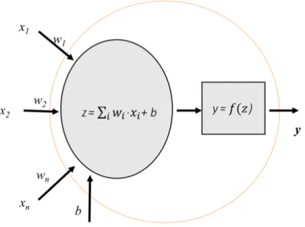
A Neural Network (NN) is a type of machine learning methods slightly inspired in the behavior observed in the axons of neurons in the brains. Formally, a NN is an information-processing structure that takes the form of a directed graph where the nodes are neurons and the edges are connections. A neuron is a local computing device that gets an input vector, combines this vector with the local parameters (weights and bias) and outputs a scalar quantity as a result. The output can be part of the final NN result or can be delivered as part of the input of another connected neuron.
A simple neuron can be defined in a more detailed way separating its behavior in three parts:
• Input: The input of a neuron is composed of three elements:
– x∈Rn : the vector of inputs from the previousnneurons.
– w∈Rn : the vector of weights of the neuron inputs.
– b∈R: the bias of the neuron.
Figure 3.1: A graphical representation of the sigmoid function and the hyperbolic tangent (tanh) function. Source: http://ronny.rest/blog/
of the activation function. Normally, the neuron statez is computing with the Equation 3.1.
z=X
i∈n
wixi+b (3.1)
• Activation function: Finally, an activation function f() is applied to the result of the previous combination and the result of this function is the output y of the neuron. Typically, the sigmoid and the hyperbolic tangent (tanh) functions are the most used (Figure 3.1).
Figure 3.2 shows a generic schema of a neuron with the three mentioned parts.
The basic structure of a NN is composed of different layers of neurons. Typically, the neurons of a layer are only connected to the neurons of the next layer. It exists three different kinds of layers:
• Input layer: The first layer of a NN is the input layer, which represents the input of the model. Usually, this layer is not counted given that it does not perform any operation and its output is simply the input.
• Output layer: The last layer of a NN is the output layer, which computes the final result of the model using a neuron for each output variable.
• Hidden layer: The remainder layers are the hidden layers.
Figure 3.3 shows the basic schema of a simple NN with the three different mentioned types of layers. A NN with more than one hidden layer is considered a Deep Neural Network.
Figure 3.2: Basic schema of a simple Neuron. Source: https://torres.ai/
Figure 3.3: Basic schema of a simple Neural Network. Source:
Figure 3.4: Schema of an unrolled Recurrent Neural Network. Source: http://colah.github.io/
3.2
Recurrent Neural Networks
The networks whose directed graph does not contain cycles are considered feed-forward Neural Networks (this is the traditional neural networks approach). Against, the networks whose graph contains cycles are called Recurrent Neural Networks (RNN). Although it seems a completely different schema, if the cycle is unrolled the RNN can be considered as multiple copies of the same network, each passing a message to a successor. Figure 3.4 shows an unrolled RNN diagram whereA represents the repeating part of NN andxtis some input that outputs a valueht.
Contrary to the human thinking process, the feed-forward Neural Networks start each process from a scratch state. Many problems related to sequences and lists can use the previous states in order to improve the results for the next ones. In this way, RNN allows information to be passed from one step of the network to the next one, achieving to persist information between instances. Some application examples of these models are based on problems of temporal series, where this recurrent feedback takes advantage of the temporal relation between the data.
3.2.1
Long Short-Term Memory Neural Networks
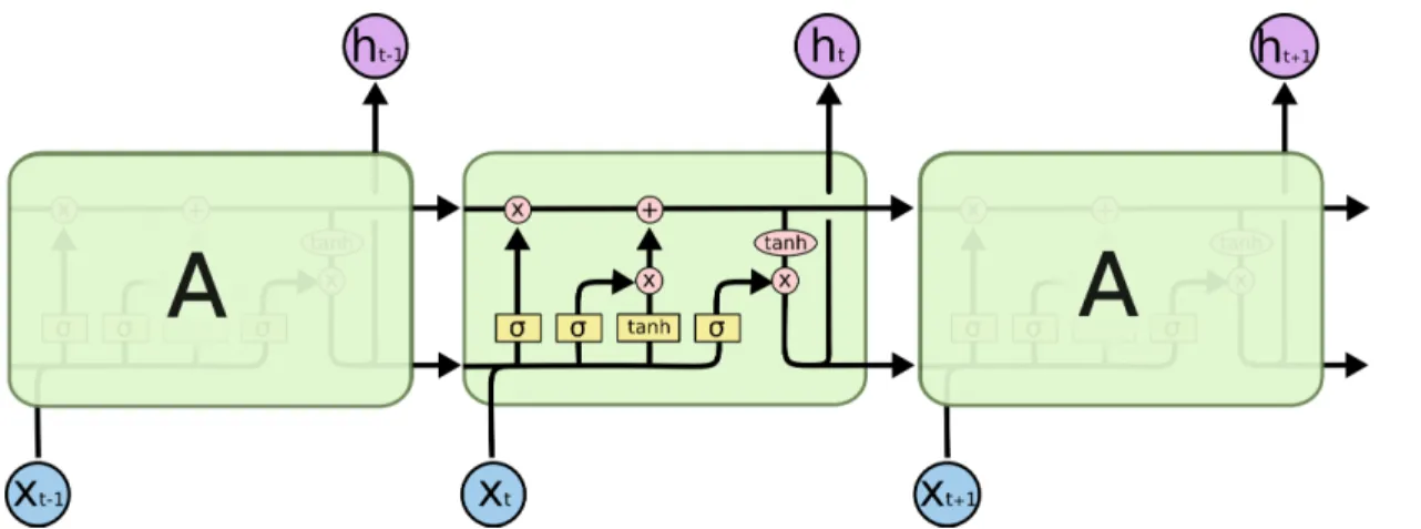
Theoretically, the simple RNNs are capable of handling “long-term dependencies”, but in practice, they do not seem to be able to learn them. To deal with this problem Hochreiter and Schmidhuber [1997] propose Long Short-Term Memory Neural Networks (LSTM), which are a kind of RNN capable of remembering information for long periods of time. The difference between the simple RNN and the LSTM is the structure of the repeating module. In standard RNNs, this repeating module will have a very simple structure, such as a single hyperbolic tangent layer. However, as it is shown in Figure 3.5, in LSTMs instead of having a single neural network layer, there are four. In order to ease the understanding of the schemas, the notation defined in Figure 3.6 is used.
The main peculiarity of the LSTMs is the double recurrent connections in the repeating module. Besides the typical recurrent connection in RNNs which reuse the output of the previous prediction, the LSTMs has the cell state (represented in the figure 3.5 by the top horizontal arrow). This cell state allows keeping cumulative information which can be modified in each execution through some minor linear interactions. The internal LSTM behavior can be explained in 4 steps:
Figure 3.5: Schema of a Long Short Term Memory network layer. Source: http://colah.github.io/
Figure 3.6: Notation of the LSTM schemas. Source: http://colah.github.io/
1. The first part in a LSTM, named forget gate (Figure 3.7), decides what information remove from the cell state. It uses a sigmoid layer that combinesht−1 (the hidden state) andxt(the input) and outputs a number between 0 (remove it completelly) and 1 (keep it completely) for each number in the cell stateCt−1 (Equation 3.2).
ft=σ(Wf·[ht−1, xt] +bf) (3.2) 2. The second one, named input gate (Figure 3.8), selects what information has to be added to the cell state. It is formed by two parts. First, a sigmoid layer usesht−1andxtand then, it generates a
Figure 3.8: The focus of the LSTM schema for the second step. Source: http://colah.github.io/
Figure 3.9: The focus of the LSTM schema for the third step. Source: http://colah.github.io/
vectoritof values between 0 and 1 (Equation 3.3). These values quantify what portion of the state values will be updated. Next, a tanh layer combinesht−1andxtto create a vector of new candidate values,Cet(Equation 3.4).
it=σ(Wi·[ht−1, xt] +bi) (3.3)
e
Ct=tanh(WC·[ht−1, xt] +bC) (3.4) 3. With the results of the previous steps, the cell state can be updated (Figure 3.9). Multiplying the old state by ft, the new cell state forgets the information selected in the first step. So, the new information from step two is added to the new state. This new information is obtained by multiply theit(which values have to be updated) andCet(the new candidates values). The full operation is in the Equation 3.5.
Figure 3.10: The focus of the LSTM schema for the fourth step. Source: http://colah.github.io/
4. The last step (Figure 3.10) is to compute the output, which is a filtered version of the updated cell state. First, a sigmoid layer decides, based inht−1 andxt, what parts of the cell state are relevant
for the output (Equation 3.6). Then, the cell state is mapped to values between−1 and 1 using a tanh multiplied by the results from the sigmoid layer (Equation 3.7).
ot=σ(Wo[ht−1, xt] +bo) (3.6)
ht=ot∗tanh(Ct−1) (3.7)
Although the described LSTM schema is one of the most adopted ones, it exists many slightly different LSTM schemas. Some of them have their own name and due to its influence in the literature are considered as different methods. One of the most popular versions is the Gated Recurrent Unit (GRU), which is a simplification of the LSTM presented by Fu et al. [2017] (Figure 3.11 and Equation 3.8). The main differences between both are:
• The GRU structure combines the forget and input gates into a single update gate.
• Also, it merges the cell state and hidden state in a single connection.
• The output of the GRU is directly the hidden state instead of being a filtered version.
zt=σ(Wz·[ht−1, xt]) rt=σ(Wr·[ht−1, xt]) e ht=tanh(W ·[rt∗ht−1, xt]) ht= (1−zt)∗ht−1+zt∗het (3.8)
![Figure 4.4: Conceptual example of the inputs I t generation. Source: Yu et al. [2017]](https://thumb-us.123doks.com/thumbv2/123dok_us/1293157.2673355/55.918.133.810.126.335/figure-conceptual-example-inputs-i-generation-source-yu.webp)