ii
Model Compression: Distilling
Knowledge with Noise-based
Regularization
Bharat Bhusan Sau
A Thesis Submitted to
Indian Institute of Technology Hyderabad
In Partial Fulfillment of the Requirements for
The Degree of Master of Technology
Under the guidance of
Dr. Vineeth N Balasubramanian
Deparment Of Computer Science and Engineering
I.I.T. Hyderabad
Model Compression: Distilling Knowledge with
Noise-based Regularization
Bharat Bhusan Sau
Indian Institute of TechnologyHyderabad, India
[email protected]
Dr. Vineeth N B
Indian Institute of TechnologyHyderabad, India
[email protected]
Abstract
Deep Neural Networks give state-of-art results in all com-puter vision applications. This comes with the cost of high memory and computation requirement. In order to deploy state-of-art deep models in mobile devices, which have lim-ited hardware resources, it is necessary to reduce both mem-ory consumption and computation overhead of deep models. Shallow models fit all these criteria but it gives poor accuracy while trained alone on training dataset with hard labels. The only way to improve the performance of shallow networks is to train it with teacher-student algorithm where the shallow network is trained to mimic the response of a deeper and larger teacher network, which has high performance. The information passed from teacher to student is conveyed in the form of dark knowledge contained in the relative scores of outputs corresponding to other classes. In this work we show that adding random noise to teacher-student algorithm has good effect on the performance of shallow network. If we perturb the teacher output, which is used as target value for student network, we get improved performance. We argue that using randomly perturbed teacher output is equivalent to using multiple teachers to train a student. On CIFAR10 dataset, our method gives 3.26% accuracy improvement over the baseline for a 3-layer shallow network.
1.
Introduction
Since the remarkable success in object recognition by the famous work of Krizhevsky et al.[12] in 2012, deep learning started to replace classical computer vision in wide variety of real-world applications. It started to give performance that was previously unachievable. However it came with certain costs. A large and deep neural network needs to be trained which requires lot of data, massive amount of com-putation power and huge memory consumption and long training time.
The state-of-art deep models are very wide as well as deep. It requires lot of space for storage. It takes good amount of
time for prediction even when we use GPUs. The actual issues start to occur when we try to deploy these state-of-art models in mobile devices. The mobile devices have limited hardware resources. It has hardly 1-2 GB of RAM, single-core processor and limited battery power. When we start to use a state-of-art deep model in a mobile device, it consumes so much memory, computation time and battery power that it becomes impractical to use deep models in mo-bile devices. To overcome these issues we must find a way to generate a deep model, which will require less memory space, computation time, battery power without sacrificing prediction accuracy significantly. So when we talk about model compression we mean either of these:
• Reducing memory consumption only
• Reducing computation overhead only
• Reducing both memory consumption and computation overhead
There are variety of techniques for model compression. We can categorize most of the model compression methods in either of the below categories:
• Replacing Fully Connected Layers:
90-95% of the parameters reside in fully connected lay-ers. Only 5-10% resides in convolutional laylay-ers. So if our goal is to reduce the model size, we can replace the fully connected layers with convolutional layers and global average pooling. Lin et al.[10] proposes such an architecture called Network-in-Network where there is no fully connected layer resulting reduced size of the model. However, it has two major drawbacks: (i) Con-volution is a costly operation. It takes much more time to evaluate than fully connected layers. Thus replacing fully connected layers with convolutional layers will de-crease model size but will inde-crease computation over-head. (ii) Feature Transfer is difficult in this method. In order to reduce training time or for small datasets, it is a common practice to take a pretrained model trained on Imagenet and finetune only the last few fully connected layers for that dataset thereby reusing the features learnt from Imagenet. As there is no fully connected layer in the NIN architecture, it is difficult to reuse the features learnt by NIN model for other tasks.
• Hashing the Weights:
Hashing the weights into several hash buckets will re-sult in less no of parameters as each hash bucket de-notes a single parameter. [14] follows this technique.
• Vector Quantization:
There are different techniques to quantize the weights resulting to less no of parameters. [15][16] are example of such methods.
• Pruning:
There are many redundant weights/neurons/filters/special locations for convolution in deep model. [17][18][19][20][21] try to explore these redundancy. These redundant things are then pruned to get smaller and faster deep model.
• Low-Rank Matrix Factorization:
This method is used to reduce parameters in fully con-nected layers. [22] proposes such a method to reduce parameters in last fully connected layer.
• Network Binarization:
Reducing the precision of floating point numbers is a way to reduce size of the model. The extreme case is network binarization, where all the weights and acti-vations are represented as +1 or -1. [23][24] proposes such method which is very fast as well as requires less memory.
• Shallow Networks:
Another approach is to train a shallow network which can give very close performance to the state-of-art model. Shallow models have less no of parameters as well as less amount of computation overhead compared to a deep network. But it is difficult to train a shal-low model which can give comparable performance to a deep model by using original hard labels only. The only way to train such a model is to use teacher-student algorithm ([5][6][7]) where the shallow teacher-student model is trained to mimic the response of a deep teacher model. The knowledge passed from teacher to student is conveyed asdark knowledgecontained in the relative scores of outputs corresponding to other classes. In this paper we aim to improve the performance of a shallow network while using teacher-student framework. We pro-pose to perturb the output from teacher which is used as target value for student. Before going into details of our method, we need to review the teacher-student framework, also known as Dark Knowledge method.
2.
Teacher-student training method
2.1
Introduction to Dark Knowledge:
The teacher-student training method was first proposed by Bucilu et al. [5] where they created synthetic data by labeling unlabelled data with a teacher model. This syn-thetically labeled data is then used to train a smaller stu-dent model. The synthetically labeled data contains the knowledge represented by the teacher model. Ba Caru-ana[7] proposed to train the student model by mimicking the logit values of teacher model.
Hinton et al.[6] generalized this method by introducing a temperature variable in softmax function. They showed that softened output at higher temperature conveys much impor-tant information. They termed this information which is expressed by the relative scores(probabilities) of the output classes as dark knowledge. Urban et al(2016)[8] argued that
training on the logarithms of predicted probabilities (logits), provides the dark knowledge that helps students by placing emphasis on the relationships learned by the teacher model across all of the outputs. This is the spirit of the definition of dark knowledge we are using in this paper.
2.2
Advantage of Dark Knowledge:
We get following advantages while training a shallow net-work with dark knowledge over training it with original 0/1 hard labels:
• Small amount of training data is sufficient to train the shallow network.
• Convergence is faster than using hard labels only.
• Dark knowledge works as powerful regularizer for the student model as it provides lot of helpful information contained in the soft target.
• Without using dark knowledge we cannot train a shal-low model of comparable accuracy.
3.
Main idea: noise-based regularization of
stu-dent networks using dark knowledge
In dark knowledge method, output of teacher network is used as the target value for student network. In this paper, we propose to perturb the teacher network output with zero-mean gaussian noise and use that perturbed value as the target value for student network. We show that adding noise to teacher output has great effect on training of student. This is equivalent to not only using noisy data for training but also using multiple teachers for training same student network.
We chose the logit matching method of Ba Caruana[7] for our tests. We perturb the logit values of teacher and use it as target values for student. Loss function is Euclidean loss between student logits and perturbed teacher logits.
Why Noise: Regularization is important to improve the generalization ability of neural network. Noisy training data is a good regularizer as it prevents overfitting of the network. It is experimentally shown that adding noise to training data can lead to improved network generalization[1]. Bishop[2] showed that training with noisy data is equivalent to adding noise to loss function. In our work, we add noise to teacher logits. This noise is then propagated to loss layer while calculating Euclidean loss. Thus it works as adding noise to training data. However, this is not the only effect of noise. The noisy logit output of teacher network not only prevents overfitting of the student network but also feeds different target value for same training data in different epochs. In other words, the student model see different target value for same training data in every epoch, which is equivalent to use many teachers for training one student network. The no of teachers in this case will be equal to the no of training epochs. This makes the student to learn better and prevents from overfitting to single teacher.
4.
Background
Earlier efforts in teacher-student network learn-ing: The first work of teacher-student algorithm was done by Bucilu et al.[5] where they created synthetic data by la-beling unlabelled data with a teacher model. This synthet-ically labeled data is then used to train a smaller student
model. Ba & Caruana[7] provided a method to train by mimicking the logit values. Euclidean loss is used as the loss function. Hinton et al.[6] provided a general method to train a student model by introducing temperature variable in softmax function. At very high temperature this is equiv-alent to matching logits. The teacher-student algorithm is not used for training a shallow network only. It can also be used for training a thin and deep network. Romero et al.[9] proposed to use intermediate hidden layer output as target value for training a thin and deep net.
Noise as Regularizer: Using noise as regularizer is a old trick. Sietsma et al.[1] experimentally demonstrated that training with noise-distorted input improves general-ity of the network. Bishop[2] proved that minimization of sum-of-squares error with zero-mean gaussian noise(added to training data) is equivalent to minimization of sum-of-squares error without noise with a added regularized term. Neelakantan et al.[3] have shown that adding gaussian noise to first order gradients while training very deep networks can improve the performance of the very deep network. Re-cently, theDisturbLabel[4] paper has shown that randomly changing the labels of some portion of the training data on the loss layer in each mini-batch(assuming the ground truth labels are correct) gives superior result than using the orig-inal labels only.
5.
Proposed methodology
We build our work on logit matching framework[7]. Be-fore describing the proposed method we need to review this framework.
5.1
Logit Matching: Mimic Learning via
Re-gressing Logits:
In this method, the student model is trained directly on the log probability values z, also called logits, before the softmax activation. This method is a special case of Hin-ton’sKnowledge Distillation[6] method. They showed that when value of temperature is very high in softmax function, it boils down to matching logits of teacher and student. As per the argument given in Urban et al. [8], training stu-dent with logits of teacher is also a dark knowledge method. We describe this mathematically as below:
The student is trained as a regression problem given train-ing data{(x(1), z(1)), ...,(x(T), z(T))}:
L(W, β) = 1/(2∗T)X||g(x(t);W, β)−z(t)||22...(1)
where,
x(t)is training data sample/input feature
z(t)is logit output of teacher
W is the weight matrix between input features and hidden layer of student model,
βis the weights from hidden to output units,
g(x(t);W, β) is the student model prediction onx(t)
5.2
Our method: Noise-based Regularization
of Logits:
We propose to add zero-mean gaussian noise to logit layer(the layer before softmax layer) of teacher model and use this noisy logit output for training student model.
Let say, ξ is gaussian noise with mean µ and standard deviationσ. In our experiments,µ= 0 and σ∈[0.1, 1.0].
Dimension ofξis equal to the no of classes/logits.
If z(t) is the logit layer output oftthtraining sample from teacher model, then we modify it as follows:
znois(y t)
= (1 +ξ)∗z(t)
Then loss function (equation (1)) changes to
-L(W, β) = 1/(2∗T)X||g(x(t);W, β)−znois(yt)||22...(2)
There is another way of adding noise in this framework. We can add noise to logit layer of student model instead of teacher model. Then the loss function becomes:
L(W, β) = 1/(2∗T)X||(1 +ξ)∗g(x(t);W, β)−z(t)||2 2...(3)
Multiplying the logits with (1 +ξ) implies that we are per-turbing the logit output by (100∗ξ)%
5.3
Adding Noise to Loss Layer is a
Regular-izer:
It is experimentally[1] proved that using noisy data is a way of regularization. Bishop[2] proposed an alternate way of adding noise. He showed that using zero-mean gaussian noise in training data is equivalent to adding a regulariza-tion term in loss funcregulariza-tion. In other words, we dont need to add noise in input layer. Instead we can add a regularization term to loss layer which will work same as using noisy train-ing data. Thus in our case also, minimiztrain-ing the regularized loss function is equivalent to using noisy data for training.
6.
Experiments, results and analysis
Datasets:We evaluate our method on two popular datasets. These are: MNIST[25] for handwritten digit recognition andCIFAR10[26] for image recognition.
Fixed Parameters: We use batch of size 64 for all our tests. The update rule we use is ADAM[13], which is a vari-ant of SGD. ADAM gives faster convergence and requires less tuning of learning rate. No of training epochs for all tests on MNIST is 384 and CIFAR10 is 256. Except section x.x, on all tests, we perturb the logit output of almost 50% data, i.e., in each batch logit output of 50% of the data are unchanged and logit output of rest 50% is changed accord-ing to the random gaussian value. The data samples are selected with dropout=0.5 and then logit output of those data are perturbed.
Fixing Randomness: In order to fix the randomness in all experiments, we fix the seed number to 1.
6.1
Basic Results on MNIST:
MNIST[25] is a very popular dataset for handwritten digit recognition. It has 10 classes(0-9). Training set contains 50000 images and validation set contains 10000 images. All the samples are 28x28 grayscale images. No preprocessing
Figure 1: CIFAR10 base result.
is done on the training data.
The teacher net is modified version of LeNet[11].
The architecture is : [C5(S1P0)@20-MP2(S2)]-[ C5(S1P0)@50-MP2(S2)]-FC500-FC101
The teacher net is trained on original training data with-out any noise/data augmentation and achieved 68 test er-rors.
The student net consists of two fully connected layers. Its architecture is : FC800-FC800-FC10 .
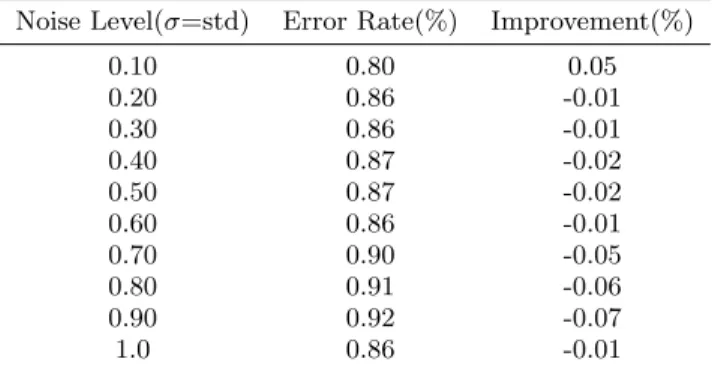
The student model achieves 85 errors when trained with logit matching without noise. When trained with noise in logit output of teacher, it achieves 80 errors. So in this case the improvement is marginal.
Detailed output is showed inTable 1.
Table 1: Result on MNIST (Noise added to Teacher)
Noise Level(σ=std) Error Rate(%) Improvement(%)
0.10 0.80 0.05 0.20 0.86 -0.01 0.30 0.86 -0.01 0.40 0.87 -0.02 0.50 0.87 -0.02 0.60 0.86 -0.01 0.70 0.90 -0.05 0.80 0.91 -0.06 0.90 0.92 -0.07 1.0 0.86 -0.01
6.2
Basic Results on CIFAR10:
CIFAR10[26] is a very popular dataset for small-scale im-age recognition. It has 10 classes: airplane, automobile, bird, cat, deer, dog, frog, horse, ship, truck . Training set has 50000 images and testing set has 10000 images. All the samples are 32x32 color images. We increased the no of
1C = Convolution Filter, S = Stride, P = Padding, MP =
Max Pooling, FC = Fully Connected
Figure 2: CIFAR10: noise in teacher vs noise in student.
Figure 3: CIFAR10: Performance with variation of noisy data percentage.
Figure 5: CIFAR10: Different student network.
Figure 6: CIFAR10: Different teacher network.
Figure 7: CIFAR10: Test with batchnorm layer.
training samples to 100000 by taking mirror image of each training sample. Other than this there is no preprocessing. The teacher net is a Network-in-Network[10] model. The ar-chitecture is: [C5(S1P2)@192] - [C1(S1P0)@160] - [C1(S1P0) @96MP3(S2)] D0.5 [C5(S1P2)@192] [C1(S1P0)@192] -[C1(S1P0)@192-AP3(S2)] - D0.5 - [C3(S1P1)@192] - [C1(S1P0) @192] - [C1(S1P0)@10] - AP8(S1)
Trained on 100000 training data it gives 9.4% error rate. Student net here is a modified version of LeNet[11], which has two convolutional layers and one fully connected layer. We opted for this student architecture based on the re-sult shown by Urban et al. [8]. They showed that in or-der to mimic a large convnet and achieve significant per-formance, the student layer must have some convolutional layers. Hence we decided to have two convolutional layers in our student architecture.
The architecture of student is: [C5(S1P2)@64-MP2(S2)]-[C5(S1P2)@128-MP2(S2)]-FC1024-FC10
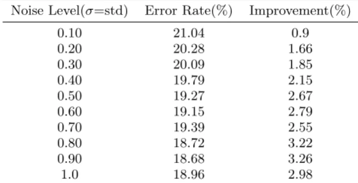
The student model achieves 21.94% error rate when trained with logit matching without noise. When trained with noise in logit output of teacher, it achieves 18.68% errors. Thus, in this case the improvement is 3.26% , which is significant. Detailed output is showed inTable 2.
Table 2: Result on CIFAR10 (Noise added to Teacher)
Noise Level(σ=std) Error Rate(%) Improvement(%)
0.10 21.04 0.9 0.20 20.28 1.66 0.30 20.09 1.85 0.40 19.79 2.15 0.50 19.27 2.67 0.60 19.15 2.79 0.70 19.39 2.55 0.80 18.72 3.22 0.90 18.68 3.26 1.0 18.96 2.98
6.3
Additional Tests on CIFAR10:
For all the tests, we added noise to teacher logits only. We do test the following:
• Comparison of noise in teacher vs noise in student
• Performance with variation of noisy data percentage
• Compare against dropout
• Different student network
• Different teacher network
• Random Noise in each iteration
• Test with batchnorm layer
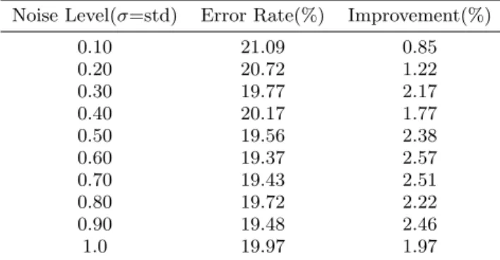
In all the basic tests we added noise to the logits of teacher only. However, in teacher-student learning framework there are two places to add noise : one in teacher output, an-other in student output. In this section we add noise to logit output of student instead of teacher. We modify it the same way we modified the teacher outputs. The result is given inTable 3. We get 2.57% improvement in performance over the base case. Although this improvement significant, it is not as good as previous case where we added noise to teacher outputs. We analyse this in section 7.2 .As adding noise to teacher output gives superior performance than adding noise to student output, we add noise to teacher outputs only for all the remaining exper-iments.
Table 3: Result on CIFAR10 (Noise added to Stu-dent)
Noise Level(σ=std) Error Rate(%) Improvement(%)
0.10 21.09 0.85 0.20 20.72 1.22 0.30 19.77 2.17 0.40 20.17 1.77 0.50 19.56 2.38 0.60 19.37 2.57 0.70 19.43 2.51 0.80 19.72 2.22 0.90 19.48 2.46 1.0 19.97 1.97
Performance with variation of noisy data percent-age:
In this section, we vary the percentage of noisy data in each batch during training and accordingly note the result. The result is given in theTable 4. For this test, we keptσ
= 0.6 constant for all the experiments. We see that per-formance improved till we corrupted 80% of teacher outputs in each batch, indicating that higher amount of noisy data improves the performance.
Table 4: Amount of Noisy Data (Noise added to Teacher)
Amount of Noisy Data(%) Error Rate(%)
10 20.09 20 19.73 30 19.39 40 19.42 50 19.15 60 19.05 70 19.04 80 18.93 90 19.0 100 19.0
Compare against dropout:
Adding noise during training is a old trick to do regu-larization. For our method, the process of adding noise is different than other methods as we are adding noise in teacher-student learning framework. As this method helps to regularize student model better, we try to verify if the
modern methods of regularization like dropout, weight de-cay are also effective in teacher-student learning framework. In this section we test the effect of dropout on student per-formance. We add a dropout layer after the fully connected layer. The result is given in Table 5. From the result we see that dropout have adverse effect on the performance of student till dropout ratio= 0.5 . However, after that, the performance improved slightly but it not comparable to our method.
Table 5: Effect of Dropout
Dropout Ratio Error Rate(%) Improvement(%)
0.1 26.48 -4.54 0.2 25.34 -3.4 0.3 24.11 -2.17 0.4 23.25 -1.31 0.5 22.46 -0.52 0.6 21.15 0.79 0.7 20.95 0.99 0.8 20.41 1.53 0.9 22.18 -0.24
Different student network:
Different teacher network:
Random Noise in each iteration:
Test with batchnorm layer:
Compression Ratio:
7.
Discussions
Why noisy logits work better:
If we perturb logits of teacher/student, it contributes some noise in loss function. As showed by Bishop[2], adding noise in loss layer is an alternate way of adding noise in training data. Noisy training data works as regularizer. Thus noisy logits work as regularizer for training the student network.
Why noise in teacher is more effective than noise in student:
We see from the experimental results that, noisy logits of teacher is more effective than noisy logits of student. The difference of highest performances between these two cases is x% for the basic student model we used.
For each training data, its teacher logit output is distorted randomly in each epoch, giving different target value to
stu-dent net for the same training data. This is equivalent to use different teacher in each epoch. The number of teachers is equal to number of epochs. As the student see differ-ent teacher in each epoch, it finds it hard to overfit to any teacher output.
We can find some analogy to this:
• If a teacher teaches a student one subject in many different way then student can learn better. It will not let the student to overfit on one particular data.
• This can also be interpreted as many teacher teaching the same subject to the student because of different target value for same training data. The no of teachers is equal to no of epochs.
• As teaching style of every teacher is unique, student will get better understanding of the subject.
8.
Conclusions
We explored the effects of noise in training student model by adding noise in various way in the teacher-student frame-work. We experimentally showed that noisy logits in teacher-student algorithm works as a powerful regularizer. We also found that higher amount of noise in logits works better. However, the biggest finding is that, noise in teacher is more effective than noise in student.
9.
Future works
Due to lack of time, we are yet to test the following: 1. Test on a large-scale image recognition database like
Imagenet.
2. Annealed Gaussian Noise(Reduced Gaussian noise with time) vs fixed Gaussian noise
3. Varying percentage of perturbed data in each iteration
References
1. J. Sietsma, and R. Dow. Creating artificial neural net-works that generalize. InNeural Networks, 1991. 2. C. Bishop. Training with noise is equivalent to tikhonov
regularization. InNeural Computation, 1995.
3. A. Neelakantan, L. Vilnis, Q. Le, I. Sutskever, L. Kaiser, K. Kurach, and J. Martens. Adding gradient noise improves learning for very deep networks. In arXiv preprint arXiv:1511.06807, 2015.
4. L. Xie, J. Wang, Z. Wei, M. Wang, and Q. Tian. Dis-turbLabel: Regularizing CNN on the Loss Layer. In
CVPR, 2016.
5. C. Bucilu, R. Caruana, and A. Niculescu-Mizil. Model compression. InKDD, 2006.
6. G. Hinton, O. Vinyals, and J. Dean. Distilling knowl-edge in a neural network. InNIPS Workshop, 2014. 7. J. Ba, and R. Caruana. Do deep nets really need to
be deep?. InNIPS, 2014.
8. G. Urban, K. Geras, S. Kahou, O. Aslan, S. Wang, R. Caruana, A. Mohamed, M. Philipose, and M. Richard-son. Do deep convolutional nets really need to be deep (or even convolutional)?. InICLR, 2016.
9. A. Romero, N. Ballas, S. Kahou, A. Chassang, C. Gatta and Y. Bengio. Fitnets: Hints for thin deep nets. InICLR, 2015.
10. M. Lin, Q. Chen, and S. Yan. Network in network. In
ICLR, 2014.
11. Y. LeCun, J. Denker, D. Henderson, R. Howard, W. Hubbard, and L. Jackel. Handwritten Digit Recogni-tion with a Back-PropagaRecogni-tion Network. InNIPS, 1990 12. A. Krizhevsky, I. Sutskever, and G. Hinton. Ima-geNet Classification with Deep Convolutional Neural Networks. InNIPS, 2012.
13. D. Kingma, and J. Ba. Adam: A method for stochastic optimization. InICLR, 2015.
14. W. Chen, J. Wilson, S. Tyree, K. Weinberger, and Y. Chen. Compressing neural networks with the hashing trick. InICML, 2015.
15. Y. Gong, L. Liu, M. Yang, and L. Bourdev. Compress-ing deep convolutional networks usCompress-ing vector quanti-zation. InarXiv preprint arXiv:1412.6115, 2014. 16. G. Soulie, V. Gripon, and M. Robert. Compression
of deep neural networks on the fly. InarXiv preprint arXiv:1509.08745, 2015.
17. S. Han, J. Pool, J. Tran, and W. Dally. Learning both weights and connections for efficient neural networks. InNIPS, 2015.
18. S. Leroux, S. Bohez, C. Boom, E. Coninck, T. Verbe-len, B. Vankeirsbilck, P. Simoens and B. Dhoedt. Lazy Evaluation of Convolutional Filters. InarXiv:1605.08543, 2016.
19. M. Figurnov, D. Vetrov, and P. Kohli. Perforated CNNs: Acceleration through elimination of redundant convolutions. InICLR, 2016.
20. S. Srinivas, and R. Babu. Data-free parameter pruning for deep neural networks. InBMVC, 2015.
21. S. Han, H. Mao, and W. Dally. Deep compression: Compressing deep neural networks with pruning, trained quantization and huffman coding. InICLR, 2016. 22. T. Sainath, B. Kingsbury, V. Sindhwani, E. Arisoy,
and B. Ramabhadran. Low-rank matrix factorization for deep neural network training with highdimensional output targets. InICASSP, 2013.
23. M. Courbariaux, I. Hubara, D. Soudry, R. El-Yaniv, and Y. Bengio. Binarized Neural Networks: Training Neural Networks with Weights and Activations Con-strained to +1 or -1. InarXiv:1602.02830, 2016. 24. M. Rastegari, V. Ordonez, J. Redmon, and A. Farhadi.
XNOR-Net: ImageNet Classification Using Binary Con-volutional Neural Networks. InarXiv:1603.05279, 2016.
25. Y. LeCun, L. Bottou, Y. Bengio, and P. Haffner. Gra-dient based Learning Applied to Document Recogni-tion. In Proceedings of the IEEE, 86(11):22782324, 1998.
26. A. Krizhevsky, and G. Hinton. Learning Multiple Lay-ers of Features from Tiny Images. InTechnical Report, University of Toronto, 1(4):7, 2009.