Towards Provable and Scalable Machine Learning

Doctoral Dissertations University of Connecticut Graduate School

6-17-2019

Towards Provable and Scalable Machine Learning

Jin Lu

University of Connecticut - Storrs, [email protected]

Follow this and additional works at:https://opencommons.uconn.edu/dissertations Recommended Citation

Lu, Jin, "Towards Provable and Scalable Machine Learning" (2019).Doctoral Dissertations. 2194.

Jin Lu, Ph.D.

University of Connecticut, 2019

In the recent decade, machine learning has been substantially developed and has demonstrated great success in various domains such as web search, computer vi-sion, and natural language processing. Despite of its practical success, many of the applications involve solving NP-hard problems based on heuristics. It is challeng-ing to analyze whether a heuristic scheme has any theoretical guarantee. In this dissertation, we show that if a certain structure occurs in sample data, it is possi-ble to solve the related propossi-blem with provapossi-ble guarantees. We propose to employ granular data structure, e.g. sample clusters or features describing an aspect of the sample, to design new statistical models and algorithms for two learning prob-lems. The first learning problem deals with the commonly-encountered missing data issue by formulating it as a matrix completion problem. When side features describing the data entities are available, we propose a new convex formulation to construct a bilinear model that infers the missing values based on the side features. This approach can be proved that with a much lower sampling rate than that of

the classic matrix completion methods, it can exactly recover or epsilon-recover missing values, depending on whether the side features are corrupted. A novel linearized alternating direction method of multipliers is developed to efficiently solve the proposed convex formulation. For the second learning problem, we build a new generative adversarial network (GAN) to generate data that follow a dis-tribution much closer to the true data disdis-tribution than the standard GAN when the data contains underlying clusters. The proposed model consists of multiple smaller GANs as components, each corresponding to a data cluster identified au-tomatically during the construction of the GAN. This GAN approach can recover the true distribution for every cluster if an appropriate Kolmogorov regularization is used. If the GAN complexity is regularized by smoothness with a parameter epsilon, we prove that GAN model can approximate the true data distribution with an epsilon tolerance. We use the Adaptive Momentum (ADAM) algorithm to optimize this model with scalability. The proposed two approaches essentially bring new insights and suggest new methods for provable and scalable machine learning.

Jin Lu

Master, University of Connecticut, USA, 2019 Master, Xi’an Jiaotong University, China, 2014

Bachelor, Northwestern Polytechnical University, China, 2010

A Dissertation

Submitted in Partial Fulfillment of the Requirements for the Degree of

Doctor of Philosophy at the

University of Connecticut 2019

Jin Lu

2019

Doctor of Philosophy Dissertation

Towards Provable and Scalable Machine Learning Presented by

Jin Lu, M.S., M.E.

Major Advisor Jinbo Bi Associate Advisor Alexander Russell Associate Advisor Sanguthevar Rajasekaran University of Connecticut 2019 iii

I owe thanks to numerous people for the successful completion of this thesis. First, to my supervisor Jinbo Bi, for believing in me and supporting me to achieve ever greater personal and professional growth. I will be forever grateful for your dedication to myself and the other students, and truly felt that you were always watching out for our well being both in times of success and struggle. With your help, I have immensely matured as a researcher, professional, and human being. To my committee members, Dr. Alexander Russell and Dr. Sanguthevar Ra-jasekaran. Thank you all for your insightful comments and encouragement, but also for the hard question which guided me to widen my research from various perspectives.

To Jiangwen Sun, for all his help with edits and comments in the early drafts of my several papers. Your help has been critical to my works, and you’ve been a great friend who has provided support to me both in and out of the lab.

To Tingyang Xu, Chao Shang, Guannan Liang, Xinyu Wang, and Xin Wang, for invaluable assistance in my research projects, and help with research strategy, project and time management, and improving my writing and programming skills. To Arron Palmer, Qianqian Tong, and Guoqing Chao for your help on the formu-lation and insights in letting me be more productive than I would have been on

To my Mom and Dad, for your unwavering love and support through my long time in school. You have always been wonderful for encouraging me to reach high and try hard. Your advice and encouragement have always given me drive to accomplish my dreams.

Finally, to my wife, Fei Dou. Fei, who has been my best friend and great compan-ion, loved, supported, encouraged, entertained, and helped me get through this study journey in the most positive way.

1. Introduction . . . 1

2. Matrix Completion with Side Information . . . 6

2.1 Introduction . . . 6

2.2 The Proposed Formulation . . . 12

2.3 Recovery Analysis . . . 17

2.3.1 Sampling Rate for Exact Recovery . . . 17

2.3.2 Sampling Rate for -Recovery . . . 41

2.4 Adaptive LADMM Algorithm . . . 51

2.4.1 Algorithm . . . 51

2.4.2 Convergence Analysis . . . 56

2.5 Experimental Results . . . 63

2.5.1 Synthetic Datasets . . . 64

2.5.2 Benchmark Datasets . . . 66

2.5.3 Case Study: Inference of missing diagnostic criteria of substance use disorders . . . 68

2.6 Summary . . . 76

3. Statistical Approximation and Learning of Kolmogorov Coupled Net . . . 77

3.1 Background . . . 77 vi

3.3 Capacity Control by GP-smooth Neurons and Surrogate Kolmogorov

Complexity . . . 85

3.3.1 GP-smooth Neurons . . . 86

3.3.2 Surrogate Kolmogorov Complexity . . . 88

3.4 Recovery Analysis . . . 94 3.5 Experiments . . . 106 3.6 Summary . . . 110 4. Conclusion . . . 111 Bibliography . . . 113 vii

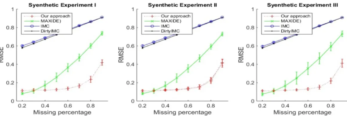
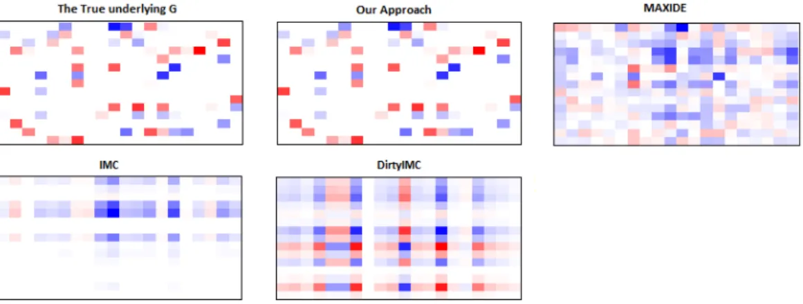
2.1 The Comparesion of RMSE for Experiments I, II, and III. . . 65 2.2 The heatmap of True G and Recovered G matrices in Experiment I. 66 2.3 HeatMap of G for MovieLens . . . 69 2.4 HeatMap of sgn(G) log(|G|) for NCI-DREAM for a better illustration 69 2.5 The recovered G by our method for the Cocaine-Opioid SUD dataset.

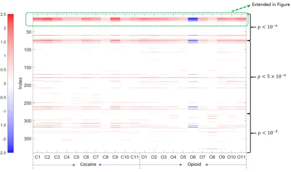
Columns C1-C11 represent 11 CUD diagnostic criteria, column-s O1-O11 reprecolumn-sent 11 OUD diagnocolumn-stic criteria. C1/O1: Larger or longer Cocaine/Opioid use than intended; C2/O2: Failed ef-forts to stop on Cocaine/Opioid; C3/O3: Much time spent in caine/Opioid related activities; C4/O4: Strong desire to use Co-caine/Opioid; C5/O5: Cocaine/Opioid effect interfered with life; C6/O6: Cocaine/Opioid use despite of its interference; C7/O7: Major activities reduced by Cocaine/Opioid use; C8/O8: Physi-cal hazard caused by Cocaine/Opioid use; C9/O9: Cocaine/Opioid use knowing it threatening health; C10/O10: Cocaine/Opioid tol-erance; C11/O11: Cocaine/Opioid withdrawal syndrome. . . 72

Opioid SUD dataset. Columns correspond to the diagnostic criteria for CUD and OUD whereas rows correspond to the candidate genet-ic variants. The right-hand side gives the locations of these genetgenet-ic

variants and their p-values obtained in the GWAS. . . 73

2.7 Gene expression distribution (RPKM, Reads per Kilobase Million) of C8orf48 across human tissues. . . 75

3.1 Synthetic experiments . . . 108

3.2 Generated results on MNIST(a), SIFA10(b) and COIL20(c). . . 109

3.3 SKC vs σ of 10 generators on MNIST dataset. . . 109

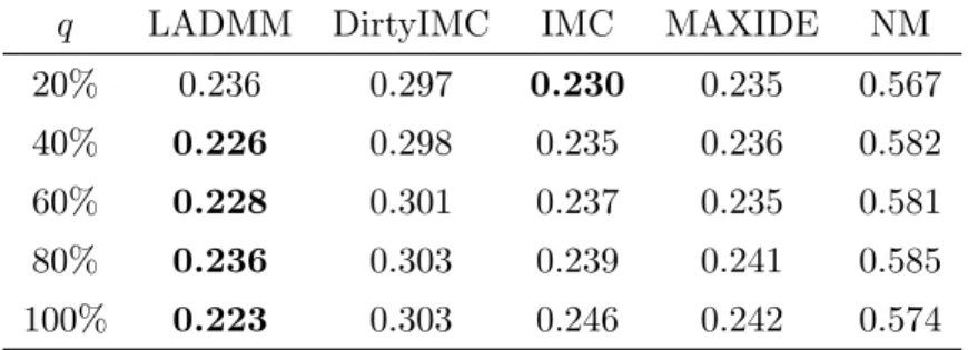
2.1 The Comparison of RMSE values of different methods on real-world datasets. . . 68 2.2 The comparison of imputation results by different methods on the

Opioid-Cocaine SUD dataset. . . 71

3.1 The Comparison of ACC values of different methods on real-world datasets. . . 107

Introduction

The momentum of research in modern machine intelligence and data analytics is towards learning from massive amounts of data. Learning via complex black-box models, such as deep learning, has seen a dramatic resurgence of popularity over the past few years because of their impressive performance on big-data problem-s. Despite their practical success, many of those machine learning methods are computationally intractable and solved on the basis of heuristics, leading to a lack of theoretical foundations and provable guarantees. As a result, there is a great need for developing scalable machine learning methods with theoretical rigor that bridge the gap between the theory and the practice.

The understanding of this gap could be revealed by the fact that compu-tational intractability only refers to the worst case inputs. Therefore, it further raises several questions. Could we design new methods that work provably on ”easier” input data? How to define and identify the ”easy” input data? Inspired by these questions, we propose practical machine learning methods with provable guarantees for several real-world learning problems in this proposal, under the

rationale that the input data has certain underlying structure.

We first consider the matrix completion problem, in which the data to be represented are in the 2nd order form such as to-user social networks and user-to-item recommender system. One typical example is the movie recommendation. In this problem, users submit ratings on a subset of movies in a database, and the vendor is required to provide recommendations based on the users preferences. Since users only rate a few movies, one would like to infer their preference for unrated items. A partially observed matrix can be defined where the rows index users and the columns index movies. With this definition, recent researches often formulate the problem as low-rank matrix completion, which recovers the matrix by assuming that similar users give similar ratings to the similar products. Besides this low-rank assumption on data, to impute missing entries, granular structures such as auxiliary or side features describing the row or column entities of the matrix are often available and useful as well. Matrix completion methods using these side features have been shown to reduce sample complexity from those classic ones that only use the observed data entries in the matrix. However, to recover a low rank data matrix, it is often assumed that the parameter matrix in their model of using the side features is also low rank, which is unnecessary. We propose a new learning formulation that constructs a bilinear model in terms of the interactions between the row and column side features to approximate the matrix entries, and requires the model parameter matrix to be sparse rather than low rank. It

is proved that when the side features span the latent feature space of the data matrix, the number of observed entries needed for an exact recovery of the data matrix is O(logn) where n is the size of the matrix. When the side features are corrupted latent features of the matrix with a small perturbation, the proposed approach can achieve an-recovery withO(logn) sample complexity. It maintains

O(n3/2_{) sample complexity similar to classic matrix completion methods if side}

features happen to be useless. A linearized Lagrangian algorithm is developed with global convergence guarantee at a linear convergence rate. Both simulation results and real-world data analyses show that the new approach outperforms the state of the art.

Then, we extend our understanding of provable machine learning to the problem of probability density estimation, which corresponds to a typical prob-lem in approximation theory and many engineering fields that aims to find an approximate solution to the problem

min

q∈Qdist(p, q)

given a hypothesis space Q of functions and given p is the function one needs to approximate. Recent needs of machine learning call for consideration of the above infinite dimensional optimization problem. Especially the mixture models for probability density estimation, as a crucial topic in unsupervised learning, are often developed to discretize a complex probability density function (pdf) p into several distributions, each of which corresponding to a cluster via new

parame-terization. As a powerful discretization technique to reveal the patterns of data without labels or humans’ representation, mixture models has been successful-ly applied to various research fields. Existing explicit mixture models typicalsuccessful-ly approach the targeted distribution by assuming thatpdfs inQfollow specific an-alytic forms [1, 2, 3, 4], or find an intermediate function embedding the samples that follow certain analytical distributions in the embedding space. Though being successful in tractable cases, as data explodes rapidly in the most recent decades, the former methodology might restrict a model’s capacity to approximate clusters with complicated distributions. It is challenging as well to determine the em-bedding function for the later methodology, which depends highly on the expert domain knowledge [5] and model selection [6]. Alternatively, aiming to implicit-ly approximate the probabilistic distribution, generative adversarial models have been enjoying considerable success as a framework of implicit germinative models for numerous types of tasks and datasets in recent years. However, quantifying the expressive power of deep generative models has not been substantially studied. In this proposal, we propose a novel metric for GAN’s capacity from approxima-tion theory, named as Surrogate Kolmogorov Complexity. By assuming the local grouping structure (mixtures) of the data, we propose a new direction to approxi-mate the data distribution by functions drawn from a function spaceQwhereQis generalized to include functions induced by a generative adversarial network and we apply the Surrogate Kolmogorov Complexity to effectively control the

capac-ity of Q. The resultant model, named Kolmogorov Coupled Nets, can provably recover the true mixtures as well as approximating both individual mixtures’ dis-tributions and the overall data distribution with a controllable tolerance, showing that the new way offers better expressive power ofQ.

Matrix Completion with Side Information

2.1 Introduction

Matrix completion is an problem of recovering or imputing missing entries in a matrix. It is commonly used to complete a data matrix when prior knowledge about the data is available, such as correlated data that lead to a low rank data matrix. It has become a fundamental technique in many engineering and scientif-ic domains, such as information retrieval [7], collaborative filtering [8], computer vision [9, 10, 11], recommender systems [12], control systems [13] and signal pro-cessing [14]. Among the numerous applications, creating a movie recommender system has been an exemplar illustration based on a numerical matrix filled with the ratings from a group of users for a set of movies. Each row of the matrix represents a user, and each column represents a movie. A recommender system aims to perform the task of predicting the preferences of users to certain movies based on limited observed ratings or reviews.

A certain relationship among data entries in the matrix is typically assumed.

Then the observed data and this relationship form a basis to impute missing en-tries. Otherwise, a matrix completion method can have infinitely possible solu-tions to guess the full matrix. For instance, a recommender system is created based on an assumption that similar users give similar ratings to similar product-s, which leads to rating correlations. These correlations are the basis for drawing the inferences regarding missing ratings. Thus, matrix completion is formulated as an optimization problem to impute the missing entries with values that yield a minimal rank of the completed matrix. However, the rank minimization problem is not convex and can be difficult to solve. By relaxing the matrix rank to its convex surrogate, which is the nuclear norm of the matrix, a convex optimization problem can be formulated. As in classical low-rank matrix completion methods [15, 16, 17], it solves the following optimization problem

minEkEk∗, subject to RΩ(E) =RΩ(F), (2.1)

where F ∈ _Rn1×n2 _{is the partially observed low-rank matrix (with a rank of r)}

that needs to be recovered, Ω ⊆ {1,· · · , n1} × {1,· · · , n2} be the set of indexes where the corresponding components in F are observed, the mapping RΩ(M):

Rn1×n2 →

Rn1×n2 _{gives another matrix whose (i, j)-th entry is M}

i,j if (i, j) ∈Ω,

or 0 otherwise, and kMk∗ computes the nuclear norm of M which is the sum of all singular values of M. Eq.(3.1) is now convex, and the advantage of working with a convex problem is that any local minimum is in fact the global minimum and thus they can be solved exactly and efficiently. Researchers have developed

first order algorithms, including the singular value thresholding (SVT) algorithm [18] for the formulation (3.1) and several variants of the proximal gradient method for solving (3.1) when noise is concerned in the observation of F [16, 19]. The proximal gradient method has been established for the noisy matrix completion with linear convergence [20, 21].

Alternatively, instead of assuming that the matrix E is low rank, studies in [22, 23] consider a decomposition of F into a product of two smaller matrices

ABT, where A ∈ _Rn1×r_{, B ∈}

Rn2×r. In this case, the optimization problem is often formulated as the minimization of the Euclidean distance betweenABT and

Fon the observed entries, and then the low-rank requirement is automatically ful-filled (i.e., rank(F)≤r). Such a matrix factorization model has long been used in many other areas, such as principle component analysis (PCA) [24]. It has several noticeable advantages in practice, such as, the compact representation of the un-known matrix, which reduces the storage space and the per-iteration computation cost. It is also elaborated that the factorization model can be easily modified to incorporate additional application-specific requirements [25]. However, there are two fundamental challenges of the factorization based models: (1) obtaining the best rank r is often intractable; (2) the non-convexity of the related optimization problem makes it difficult to guarantee that a global minimum is acquired in the recovering of the data matrix, unless the optimization starts from an initialization that is close enough to the global minimum.

Early theoretical analysis [26, 27, 28] proves that O(nrlog2n) entries are sufficient for an exact recovery of F if the observed entries are uniformly sam-pled at random where n= max{n1, n2}. Another work [29] deals with noisy data

observations in matrix completion and reveals a similar sampling rate. The ap-proach in [17] studies the matrix recovery from very few observed data entries and derives an effective algorithm that can retrieve F with a high probability and a small relative mean square error using O(rn) observed entries and further with

O(nlogn) data entries, it can retrieve the exactF. However, these bounds assume that the observed entries are sampled uniformly at random. For sample complexi-ty in a distribution-free manner, Shamir and Shalev-Shwartz [30] recently showed that O(n3/2_{) entries are sufficient for -recovery, which means the the expected}

recovery error for each entry is less than a small tolerance >0.

Recent studies start to explore side information for matrix completion [31, 32, 33, 34]. For example, to infer the missing ratings in a user-movie rating matrix, descriptors of the users and movies are often known and may help to build a content-based recommender system. For instance, kids tend to like cartoons, so the age of a user likely interacts with the cartoon feature of a movie. When few ratings are known, this side information could be the main source for completing the matrix. Based on empirical studies, several works found that side features are helpful [32, 34, 35, 36] via matrix factorization formulations; Berg et al. [37] imposes a Graph Convolutional Network representing the bipartite graph between

features of users and movies [37]. Monti et al. [38] constructs two GCNs, each extracting features of users and movies, respectively; however, all the mentioned methods above involve highly non-convex optimization, in consequence of extreme difficulty of theoretical recovery analysis.

Three recent methods have focussed on convex nuclear-norm regularized objectives, which leads to theoretical guarantees on matrix recovery [39, 40, 41]. These methods all construct an inductive model XGYT so that RΩ(XGYT) =

RΩ(F) where the side matrices X and Y consist of side features, respectively,

for the row entities (e.g., users) and column entities (e.g., movies) of a (rating) matrix. This inductive model has a parameter matrix G which is either required to be low rank [39] or to have a minimal nuclear norm kGk∗ [40]. Recovering

G of a (usually) smaller size is argued to be easier than directly recovering the matrix F. With a very strong assumption on ‘perfect’ side information, i.e., both

Xand Yare othornormal matrices and respectively in the latent column and row space of the matrix F, the method [40] is proved to have much reduced sample complexityO(logn) for an exact recovery of F. Because most side featuresX and

Y are not perfect in practice, a very recent work [41] proposes to use a residual matrix Nto handle the noisy side features. This method constructs an inductive model XGYT +Nto approximateFand requires both Gand Nto be low rank, or have a low nuclear norm. It uses the nuclear norm of the residual to quantify the usefulness of side information, and proves O(logn) sampling rate for an

-recovery when X and Y span the full latent feature space of F, and o(n) sample complexity when X and Y have noise features not from the latent space of F. An -recovery is defined as that the expected discrepancy between the predicted matrix and the true matrix is less than an arbitrarily small >0 under a certain probability.

Comparing with the recent works, our contributions are summarized as fol-lows:

(i) We propose a new formulation in [42] that estimates both E and G by imposing a nuclear-norm constraint onEbut a general regularizer on G, e.g., the sparse regularizer kGk1. The proposed model has theoretical recovery guarantees depending on the quality of the side features: (1) when X and Y are full column rank and span the entire latent feature space of F(but are not required to satisfy the much stronger condition of being orthonormal as in [40]),O(logn) observations are still sufficient for our method to achieve an exact recovery of F. (2) When the side matrices are not full rank and corrupted from the original latent features of F, i.e., X and Y do not contain enough basis to exactly recover F, O(logN) observed entries are sufficient for an -recovery.

(ii) A novel linearized alternating direction method of multipliers (LADM-M) is developed to efficiently solve the proposed convex formulation. Existing methods use side information are solved by a standard block-wise coordinate de-scent algorithm; This algorithm has convergence guarantee to a global minimum

when the optimization problem is strictly convex, or converge to a stationary point when the problem is non-convex and non-differentiable while each subproblem has unique solution [43]. Our LADMM achieves the global minimum and has a linear convergence rate [44].

(iii) Prior methods focus on the recovery ofF, and little light has been shed to understand whether the interactive model of G can be retrieved. Because of the explicit use ofEandG, our method aims to directly recover both. The unique

G in the case of exact recovery of F can be obtained by our algorithm. When

G is not unique in the -recovery case, our algorithm converges to a point in the optimal solution set.

(iv) Our proposed method demonstrates high effectiveness of integrating genotype data with other relevant sources of information for imputing missing phenotypes than other matrix completion methods [45, 46]. As an additional benefit, the proposed method constructs a bi-linear predictive model that can can help to identify important interactions that link specific genotypes to diagnostic criteria.

2.2 The Proposed Formulation

Assume that there are a side features xdescribing a user (row entity of F) and b

side features y describing a movie (column entity of F). Thus, two side feature matrices X of size n1×a and Y of size n2×b are available. To complete F, we

propose to build a predictive model, as a function ofX andY, that is constructed from the observed components of F to predict the missing ones. This is different from the transductive model commonly used in the method of Eq.(3.1) where the missing entires are directly filled rather than creating an explicit inference model. The advantage of creating a model is that the model can then be used to predict future (expanded) entries of the matrix. We can simply start with a linear model:

f =xTu+yTv+z,

where u, v, and z are model parameters. In real life applications, interactive terms between the features inXand Ycan be very important. For example, kids tend to rate animation pictures high, which means that the interactive term of age and animation genre can be a good predictor. Male users tend to rate action movies higher than female users, indicating gender-genre interaction. These inter-active terms can be informative when predicting the ratings for specific movies. Therefore, a linear model considering no interactive terms may have low predic-tive power for missing entries. We then add interacpredic-tive terms by introducing an interaction matrix Ha×b to the predictive model, which can be written as:

f =xTHy+xTu+yTv+z.

By defining ¯x = [xT _{1], ¯y = [y}T _{1] and G}(d1=a+1)×(d2=b+1) ₌

    H u vT _g    

problem can be solved to obtain the model parameter G. min

G,E g(G) +λEkEk∗,

subject to XG¯ Y¯T =E, RΩ(E) =RΩ(F),

where E is a completed version of F, ¯Xn1×d1

and ¯Yn2×d2

are two matrices that are created by augmenting one column of all ones to X and to Y, respectively, and g(G) and kEk∗ are used to incorporate the (sparsity) prior of G and (low rank) prior of E. Because the side information data can be noisy and not all the features and their interactions are helpful to the prediction of F, a sparse

G is often expected. Our implementation has used g(G) = kGk1. It is natural

to impose low rank requirement on E because it is a completed version of a low rank matrix F. The tuning parameterλE is used to balance the two priors in the

objective.

Without loss of generality and for notational convenience, we simply use

X and Y to denote the augmented matrices. Denote the Frobenius norm of a matrix by kAkF = Pn1

i=1

Pn2

j=1|ai,j|

2_{, the one norm by kAk1 =} Pn1

i=1

Pn2

j=1|ai,j|,

the nuclear norm by kAk∗ = trace(

√

ATA) and the spectral norm by kAk =

kAk2 = maxλi ∈Λ where λi is the i-th singular value in the set of all

sin-gular values Λ. The spectral norm of an operator T(A) will be denoted by

kTk = maxkAkF≤1kT(A)kF To account for Gaussian noise, we relax the

equal-ity constraint XGYT = E and replace it by minimizing their squared residual:

kXGYT −Ek2

min G,E 1 2kXGY T _−Ek2 F +λGg(G) +λEkEk∗, subject to RΩ(E) =RΩ(F). (2.2)

where λG is another tuning parameter that, together with λE, balances the three

terms in the objective. Especially, the regularizerg(·) in our formulation can take any general matrix norm and can be chosen according to any prior knowledge ofG. In our experiments, we realizedg(·) to be the`1-norm of the matrixG. In the next

section when we analyze the recovery property, we show the sample complexity needed for exact recovery when ||G||1 is used in Eq.(2.2). In the-recovery later discussed, as long as g(·) satisfies kMk∗ ≤ Cg(M), ∀M, for a constant C, so for instance g(·) can be kGk1, or ||G||F, or kGk2. Throughout this chapter,

the matrices X (and Y) refer to, i.e., either the original Xn1×a _{(and Y}n2×b_{) or}

the augmented ¯Xn1×d1

(and ¯Yn2×d2

) depending on the user-specified model. In our formulation λG influences the significance of the prior structure of G. One

can also observe that when λG is sufficiently large, the problem (2.2) regresses

to the standard matrix completion problem in [26] without side information as problem (3.1), in addition to a regularizing term in terms of kEkF equivalent to

the upper-bound prior on kEkF. Thanks to Theorem 2, a useful guidance for the hyper-parameter selection thatλG/λE = 1_n is given such that the recovery can be

achieved theoretically with certain sample complexity proposed in Theorem 2. It suggests that our formulation is more generalizable and adoptable to the standard

matrix completion in the case of no access to useful side information.

Our formulation (2.2) is different from existing methods that make use of side information for matrix completion in many different ways. Existing meth-ods [39, 40, 41] solve the problem by finding ˆH that minimizes kHk∗ subject to

RΩ(XHYT) = RΩ(F), but we expand it to include the linear term within the

interactive model. The proposed model adds the flexibility to consider both lin-ear and interactive terms, and allows the algorithm to determine the terms that should be used in the model by enforcing the sparsity in H (or G). Because

E=XGYT, the rank of G bounds that of E from above. The existing methods all minimize the rank of G (e.g. by minimizing kGk∗) to incorporate the prior of low rank E (and thus low rank F) in their formulations. However, when the rank ofGis not properly chosen during the tuning of hyperparameters, it may not even be a sufficient condition to ensure low rankE(if rank(E)the pre-specified rank(G)). It is easy to see that besides G both low-rank X and Y can lead to low-rank E as well, so a low-rank G is not necessary to result in a low-rank E. Enforcing a low-rank condition on H or G may limit the search space of the in-teractive model and thus impairing the predictive performance on missing matrix entries, which are demonstrated in our empirical results.

2.3 Recovery Analysis

LetE0 andG0 be the two matrices such thatRΩ(F) =RΩ(E0) andE0 =XG0YT.

In this section, we give our theoretical results on the sampling rate for achieving an exact recovery of E0 and G0 when X and Y are both full column rank (i.e.,

rank(X) =d1 and rank(Y) =d2) and span the latent feature space ofE0, and an

-recovery of E0 when the two side matrices are corrupted and less informative.

2.3.1 Sampling Rate for Exact Recovery

In this section, we introduce the notion of matrix coherence that measures how singular matrix columns or rows are, or in other words, how uncorrelated any columns (or rows) in the matrix can be with all other columns (or rows). Intuitive-ly, it might be easier to recover ‘incoherent’ matrices, i.e., matrices with relatively low coherence than those with high coherence. We give a few relevant definitions before presenting our results because coherence conditions are important for exact recovery of a matrix. Let F =UΣVT, X = UXΣXVTX and Y =UYΣYVTY be the singular value decomposition of F, X and Y, respectively. Without loss of generality, this decomposition only uses the non-zero eigenvalues and hence only the left and right singular vectors corresponding to non-zero eigenvalues are used inU and V. Let PU =UUT ∈Rn1×n1 PX=UXUTX =XVXΣ−X2V T XX T _∈ Rn1×n1 PV =VVT ∈Rn2×n2 PY =UYUTY =YVYΣ−Y2V T YY T _∈ Rn2×n2,

where PU, PV, PX and PY are projector matrices that project a vector onto the subspaces spanned, respectively, by the columns in U, V, X, and Y. All projectors P satisfy that P2 _=P.

Letµ0 andµ1 be the two coherence measurements for a single matrixFand

be defined as follows [26]: µ0 = max n1 r 1max≤i≤n1 kPUeik22, n2 r 1max≤j≤n2 kPVejk22 , µ1 = max i,j n1n2 r ([UV T_] i,j)2,

where ei is the unit vector with the ith entry equal to 1, which also forms the

coordinate axes when i = 1,· · · , n1. The coherence parameter µ0 measures the

alignment between the column space spanned byU(or the row space spanned by

V) and the coordinate axes. Let µ2 be the coherence measurement between two

matrices X and Y and be defined as:

µ2 = max max 1≤i≤n1 n1kxik22 d1 , max 1≤j≤n2 n2kyjk22 d2 .

where xand y are the row vectors in X and Y, respectively.

Using the above definitions, we first prove the following theorem that when

X and Y are both full column rank, (G0,E0) is the unique solution to Problem

(2.2) under two deterministic assumptions A1andA2 forF,Xand Y, and more precisely, for the projectors defined by these matrices. In several lemmas followed, we prove that with high probabilities,A1 and A2 hold. Then these probabilities help us identify a high probability, with which (G0,E0) is the unique solution to

words, with a sampling rate of O(rlogn), our method can fully recover both E0

and G0 with a high probability when X and Y are full column rank.

Theorem 1: For any matrix M ∈ _Rn1×n2_{, we define two linear operators: P}

T : Rn1×n2 → Rn1×n2 _{and P} T⊥ :_Rn1×n2 →_Rn1×n2 as follows: PT(M) = PUMPY+PXMPV−PUMPV P_T⊥(M) = (P_X−P_U)M(P_Y−P_V).

Assuming that for any M∈_Rn1×n2 _{satisfying thatM}6_{= 0, R}

Ω(M) = 0 and

M=PXMPY, we have

A1 kPT(M)kF ≤ζkPT⊥(M)k_F,

where ζ ≤qd1

2r.

We further assume that there exists a matrixH∈_Rn1×n2 _satisfyingR

Ω(H) = H such that A2 kPT(H− λG λE PQ(sgn(G0)))−UVTkF ≤ r 1 2d1 , kPT⊥(H− λG λE PQ(sgn(G0)))k< 1 2, where PQ(G) = X†GY† T by defining X† = VXΣ−X1U T X(1:d1) and defining Y † = VYΣ−_Y1UTY(1:d2), where U T X(1:d1) and U T

Y(1:d2) denote the first d1 and d2 rows of

UT_X and VT_y, respectively. Then G0 and E0 are the unique minimizer to our

optimization problem.

Assume the solution (G0,E0) is not unique, and hence there exists another

contradiction, we utilize the subgradient ofk·k∗ andk·k1 atE0 andG0 to derive a

contradiction thatλGkG0+G∆k1+λEkE0+E∆k∗ ≥λGkG0k1+λEkE0k∗. Recall the definition of a subgradient of a convex function f :_Rn1×n2 →

R. We say that

Z is a subgradient of f at E0, denoted byZ ∈∂f(E0), if

f(E)≥f(E0) +hZ,E−E0i (2.3)

for all E.

Subgradient of kEk∗: when E0 has rank r with a singular value

decom-position given by E0 = r X k=1 σkukvTk,

one can obtain that Z1 is a subgradient of kEk∗ at E0 if and only if it takes the

form Z1 = r X k=1 ukvTk +W, (2.4)

where the following two properties hold:

(i) The column space ofWis orthogonal to the linear spacespan(u1,· · · ,ur),

and the row space of W is orthogonal to span(v1,· · · ,vr).

(ii) The norm kWk is less than or equal to 1.

It is worth noting that one can derive the subgradients of the nuclear norm according to Theorem 2 in Watson [47].

Subgradient of kGk1: when G0 ∈ Rd1×d2 is sparse, we define Ω0 ⊆ {1,· · · , d1} × {1,· · ·, d2} as the set of indexes where the corresponding

compo-nents in G0 are non-zeroes, the mapping RΩ0(G): _Rd1×d2 →_Rd1×d2 gives another matrix whose (i, j)-th entry is Gi,j if (i, j) ∈ Ω0, or 0 otherwise. Then one can

obtain a subgradient ofkGk1 at G0 as follows:

Z2 = sgn(G0) +J (2.5)

where the matrixJ∈_Rd1×d2 _{can be any matrix such thatR}

Ω0(J) = 0 andkJk_∞≤ 1. The signum function on the matrix G∈_Rd1×d2 _{is defined as follows:}

sgn(Gi,j) =                    −1 if Gi,j ≤0 0 if Gi,j = 0 1 if Gi,j ≥0 ∀1≤i≤d1,1≤j ≤d2. (2.6)

In order to derive a contradiction, we illustrate several useful facts (state-ments) below:

(a) By the constraint in Eq. (2), we have RΩ(F) = RΩ(E0). If E0 =

XG0YT, we have RΩ(X(G0+G∆)YT) =RΩ(XG0YT), and X(G0 +G∆)YT =

UXUTXUXΣXVTX(G0+G∆)VTYΣYUYTUYUTY =PX(X(G0+G∆)YT)PY, asG0+

G∆ minimizes the original problem.

(b) XG∆YT 6= 0, since X

†

XG∆(YY

†

)T _{= G}

∆ 6= 0 for X and Y are full

column rank.

(c) XG∆YT = UXUXTUXΣXVTXG∆VYTΣYUTYUYUTY = PX(XG∆YT)PY and it holds that RΩ(XG∆YT) = 0.

haveXG∆YT 6= 0 with Assumption A1.

(e)U⊥ andV⊥are the left and right singular vectors ofPT(XG∆YT), while

UTU⊥ = 0 andVTV⊥= 0.

(f) SinceRΩ(XG∆YT) = RΩ(X(G0+G∆)YT)−RΩ(X(G)YT) = 0 we have

RΩ(XG∆YT) = 0.

Proof. By making use of the above statements, we have

λEkE0+E∆k∗+λGkG0+G∆k1 =λEkX(G0+G∆)YTk∗+λGkG0+G∆k1 ≥λE X(G0+G∆)YT,UVT +U⊥VT⊥ (i) +λGkG0k1+λGhsgn(G0) +J,G∆i (ii) =λE XG0YT,UVT + XG0YT,U⊥VT⊥ + XG∆YT,UVT +U⊥VT⊥ +λGkG0k1+λGhsgn(G0) +J,G∆i

The term (i) and (ii) are obtained since the inequalities are implied by the subgradients and let W = U⊥VT⊥ and J satisfy RΩ0(J) = 0 and kJk_∞ ≤ 1. Furthermore one can obtain that

λE XG0YT,UVT +XG0YT,U⊥VT⊥ +XG∆YT,UVT +U⊥VT⊥ +λGkG0k1+λGhsgn(G0) +J,G∆i =λEkE0k∗+λE XG0YT,U⊥VT⊥ +λE XG∆YT,UVT +U⊥VT⊥−H (iii) +λGkG0k1+λGhsgn(G0) +J,G∆i =λEkE0k∗+λGkG0k1+λE( P_T⊥(XG_∆YT),U_⊥VT_⊥−P_T⊥(H) (iv) +λGhsgn(G0) +J,G∆i+ PT(XG∆YT),UVT −PT(H) (v) )

where the term (iii) is obtained since we have RΩ(H) = H in Assumption A2,

and RΩ(XG∆YT) = 0 using Statement (f), so that we have

XG∆YT,H = RΩ(XG∆YT), RΩ(H) + R\Ω(XG∆YT), R\Ω(H)

= 0. The terms (iv) and (v) are derived from Statement (c). Using matrix norm inequality and selecting

J=−sgn(R\Ω0(G_∆)) so thathJ,G_∆i=kR_\Ω0(G_∆)k₁, one can derive by the norm inequality as follows: λEkE0+E∆k∗+λGkG0+G∆k1−(λEkE0k∗+λGkG0k1) ≥λGkR\Ω0(G_∆)k₁+λ_E −kPT(XG∆YT)k∗kUVT −PT(H− λG λE PQ(sgn(G0))k +kP_T⊥(XG_∆YT)k∗− kPT⊥(H− λG λE PQ(sgn(G0)))kkPT⊥(XG_∆YT)k∗ ≥λGkR\Ω0(G_∆)k₁+λ_E kP_T⊥(XG_∆YT)k∗(1− kPT⊥(H− λG λE PQ(sgn(G0)))k) − kPT(XG∆YT)k∗kUVT −PT(H− λG λE PQ(sgn(G0)))k >λGkR\Ω0(G_∆)k₁+λ_E   kPT⊥(XG∆Y T_)k ∗(1− 1 2)− √ rkPT(XG∆YT)kF r 1 2d1 (vi)    (by Assumption A2) >λGkR\Ω0(G_∆)k₁+λ_E   kPT⊥(XG∆Y T_)k ∗(1− 1 2)− √ rkP_T⊥(XG_∆YT)k_∗ r 1 2d1 (vi)    (by Statement (d)) ≥λGkR\Ω0(G_∆)k₁+λ_EkP_T⊥(XG_∆YT)k∗( 1 2 − s ζ2_r 2d1 )>0 (2.7) since kP_T⊥(XG_∆YT)k_∗(1 2 −ζ q _r

2d1) ≥ 0 which is implied from Assumption A2.

(vi) is obtained from kPT(XG∆YT)k∗ ≤

√

re-veals that the (E0 +E∆,G0 +G∆) is not the minimizer for our optimization

problem.

We need to prove that A1 and A2 hold with high probabilities (in Lemmas 1, 8, and 9. However, before going to the detailed proof, we summarize our first main result that characterizes the exact recovery as follows:

Theorem 2: Let µ= max(µ0, µ2), σ = max(kΣ−_X1k∗,kΣ−_Y1k∗), n = max(n1, n2),

q0 = 1₂(3 + logd1), T0 = 128₃ σ2pµmax(µ1, µ)r(d1+d2) lognand T1 = 8p₃σ2µ2(d1d2+

r2_{) logn, where p is a constant. Assume T}

1 ≥ q0T0, X and Y are both full

col-umn rank. For any p > 1, by setting λE/λG = _n1, with a probability at least

1−2q0n−p+1 −2q0n−p+2, (G0,E0) is the unique optimizer to Problem (2.2) with

necessary sampling rate as few as O(rlogn). More specifically, the sampling size

|Ω| should satisfy that |Ω| ≥ 64 3 σ

2_pµmax(µ

1, µ)r(3 + logd1)(d1+d2) logn.

Proof. To satisfy the probabilistic conditions that Assumption A1 and Assump-tion A2 that could holds in, one can deduce from Lemma 1, Lemma 7, Lemma 8, and Lemma 9 that |Ω| ≥ q0T0 = 64₃ σ2pµmax(µ1, µ)r(3 + logd1)(d1+d2) logn;

therefore, |Ω|=O(rlogn).

A1 holds with high probability

In this subsection we prove that Lemma 1 holds with a certain probability. Lem-ma 1 is derived by combining the results from LemLem-ma 4 and LemLem-ma 5, which

upper-boundkPT(M)kF and lower-bound kPT⊥(M)kF, and clarify the inequality between them. Lemma 2 and 3 are cited from [40] to facilitate the proof.

Let us first describe Lemma 1 as follows.

Lemma 1: With a certain probability at least 1−4n−p+1 _{for p > 1 as stated in}

Theorem 2, for anyM6= 0,M∈_Rn1×n2 _satisfyingR

Ω(M) = 0andM=PXMPY

we have

kPT(M)kF ≤ζkPT⊥(M)k_F,

where ζ is the same as in Lemma 1, if the sampling rate |Ω| can be bounded as

T0 ≤ |Ω| ≤T1. Proof. Since RΩ(M) = RΩ(PX(M)PY) = RΩPT(M) + RΩPT⊥(M) = 0, we haveRΩPT(M) =−RΩPT⊥(M). Since hPT(M),Mi=hPT(M), PT(M) + (I−PT)(M)i =hPT(M), PT(M)i+hPT(M),(I−PT)(M)i=hPT(M), PT(M)i=hM, PT(M)i, we could attainkRΩPT(M)kF2 =hRΩPT(M), RΩPT(M)i=hM, PTRΩRΩPT(M)i= hM, PTRΩPT(M)i. Therefore, we have n1n2 |Ω| hM, PTRΩPT(M)i= n1n2 |Ω| hM, PT⊥RΩPT⊥(M)i.

we have 1 2kPT(M)k 2 F ≤ n1n2 |Ω| hM, PTRΩPT(M)i ≤16σ 2_µ2_p(d 1d2+r2) logn 3|Ω| kPT⊥(M)k 2 F ≤16σ 2_µ2_p(d 1d2+r2) logn 3T0 kPT⊥(M)k2_F ≤1 4kPT⊥(M)k 2 F. Hence, we have kPT(M)kF ≤ 1 √ 2kPT⊥(M)kF ≤ r d1 2rkPT⊥(M)kF ≤ζkPT⊥(M)kF since √1 2 ≤ q d1 2r.

We recite Lemma 2, Lemma 3 that have been previously derived in [40] from the Berstein Inequality [28]. We use these lemmas in proving both Lemmas 4 and 5.

Lemma 2: [40] Let X1, ..., XL be independent zero-mean random matrices of

dimension a×b. Suppose ρ2_k ≥ max{k_E[XkXTk]k,kE[X T

kXk]k} and kXkk ≤ M

almost surely for all k. If we assume

M2log a+b ξ ≤ 3 8 X ρ2_k,

then with a certain probability at least 1−ξ, we have

k L X k=1 Xkk ≤ v u u t 8 3log a+b ξ L X k=1 ρ2 k.

Lemma 3: [40] Let X1, ..., XL be independent zero-mean random matrices of

dimension a × b. Suppose ρ2

k ≥ max{kE[XkXTk]k,kX T

kXkk} and kXkk ≤ M

almost surely for all k. If we assume

M2log a+b ξ ≥ 3 8 X ρ2_k,

then with a certain probability at least 1−ξ, we have

k L X k=1 Xkk ≤ 8 3Mlog a+b ξ .

Next we will boundkPT−n|1Ωn|2PTRΩPTkby using Lemma 2 and Lemma 3.

Lemma 4: With a certain probability at least 1−2n−p+1_{, we have}

PT − n1n2 |Ω| PTRΩPT ≤ s 8σ2_pµ2_r(d 1+d2) logn 3|Ω| if |Ω| ≥ 8 3σ 2_pµ2_r(d

1+d2) logn. Therefore, for any M∈Rn1×n2, we have 1 2kPT(M)k 2 F ≤ n1n2 |Ω| hM, PTRΩPT(M)i if |Ω| ≥T0.

Proof. To simplify the left side of the inequality, for any i∈[n1] and j ∈[n2],

define the linear operatorTi,j as

Ti,j(M) =

M, PT(eieTj)

where R(i,j)(M) = eieTjMi,j for any M ∈ Rn1×n2. From Theorem 4.1 in [26] we similarly could obtain

PTRΩPT(M) = X (i,j)∈Ω PT(M),eieTj PT(eieTj) = X (i,j)∈Ω M, PT(eieTj) PT(eieTj) = X (i,j)∈Ω PTR(i,j)PT(M) = X (i,j)∈Ω Ti,j(M)

To implement Lemma 2, we need to give M and the corresponding ρ2 k’s.

SincekPT −n_|1_Ωn_|2PTPΩPTkcan be viewed as the spectral norm of |Ω|independent

zero-mean random variables _|Ω1_|PT − n_|1_Ωn_|2Ti,j, then we have

k 1 |Ω|PT − n1n2 |Ω| Ti,jk ≤max{k 1 |Ω|PTk,k n1n2 |Ω| Ti,jk} = max{k 1 |Ω|PTk, n1n2 |Ω| arg maxkMkF=1 k M, PT(eieTj) PT(eieTj)kF} = max{k 1 |Ω|PTk, n1n2 |Ω| arg maxkMkF=1 M, PT(eieTj) kPT(eieTj)kF} = max{k 1 |Ω|PTk, n1n2 |Ω| kPT(eie T j)k 2 F}.

To bound kPT(eiejT)k2F, from the definition ofPT, we get kPT(eieTj)k 2 F =PT(eieTj),eieTj =PX(eiejT)PV,eieTj +PU(eiejT)PY,eieTj − PU(eieTj)PV,eieTj =kPX(eieTj)PVk2F +kPU(eieTj)PYk2F − kPU(eieTj)PVk2F ≤kPXeik2FkPVejk2F +kPUeik2FkPYejk2F ≤kXVXΣ−X2V T Xk 2 F d1µ2 n1 rµ0 n2 +kYVYΣ−Y2V T Yk 2 F rµ0 n1 d2µ2 n2 ≤kΣ−_X1k2 ∗ d1µ2 n1 rµ0 n2 +kΣ−_Y1k2 ∗ rµ0 n1 d2µ2 n2 ≤σ2rµ0µ2(d1+d2) n1n2 ≤ σ 2_µ2_r(d 1+d2) n1n2 . Therefore, we have k 1 |Ω|PT − n1n2 |Ω| Ti,jk ≤max{k 1 |Ω|PTk, n1n2 |Ω| kPT(eie T j)k 2 F} ≤max{k 1 |Ω|PTk, σ2µ2r(d1+d2) n1n2 } = max{ 1 |Ω|, σ2µ2r(d1+d2) n1n2 }= max{ 1 |Ω|, σ2µ2r(d1+d2) n1n2 }= σ 2_µ2_r(d 1+d2) n1n2 =M. As _|Ω1_|E[PTRΩPT] = _|Ω1_|[PTE(RΩ)PT] = _|Ω1_|[PT_n|Ω| 1n2PT] = 1 n1n2PT, the

corre-sponding ρ2_i,j can be calculated as ρ2_i,j =k_E[( 1 |Ω|PT − n1n2 |Ω| Ti,j) T₍ 1 |Ω|PT − n1n2 |Ω| Ti,j)]k =k_E[ 1 |Ω|2PTPT + n2 1n22 |Ω|2Ti,jTi,j − 2n1n2 |Ω|2 PTTi,j]k =k 1 |Ω|2PT + n2 1n22 |Ω|2E[Ti,jTi,j]− 2n1n2 |Ω|2 PTE[Ti,j]k =k 1 |Ω|2PT + n2 1n22 |Ω|2E[Ti,jTi,j]− 2n1n2 |Ω|2 PT 1 n1n2 PTk =kn 2 1n22 |Ω|2 E[Ti,jTi,j]− 1 |Ω|2PTk ≤max{n 2 1n22 |Ω|2 E[Ti,jTi,j], 1 |Ω|2PT} ≤max{n 2 1n22 |Ω|2 E[kPT(eie T j)k 2 FkTi,jk], 1 |Ω|2} ≤max{n 2 1n22 |Ω|2 σ2rµ2(d1+d2) n1n2 1 n1n2 kPTk], 1 |Ω|2} =σ 2_µ2_r(d 1+d2) |Ω|2 . By Lemma 3, with M = σ2µ2r(d1+d2) n1n2 and ρ 2 i,j = σ2_µ2_r(d 1+d2) |Ω|2 , we conclude

with a certain probability 1−2n−p+1,

kPT − n1n2 |Ω| PTRΩPTk ≤ s 8 3log n1+n2 2n−p+1 σ2_µ2_r(d 1+d2) |Ω| ≤ s 8σ2_pµ2_r(d 1+d2) logn 3|Ω|

which also should satisfy the condition that

σ4µ4r2(d1+d2)2 |Ω|2 log n1+n2 2n−p+1 ≤ 3 8 σ2µ2r(d1+d2) |Ω| which means |Ω| ≥ 8σ 2_pµ2_r(d 1+d2) logn 3 .

Moreover, if |Ω| ≥T0 ≥ 128σ 2_pµ2_r(d 1+d2) logn 3 , we have PT − n1n2 |Ω| PTRΩPT ≤ s 8σ2_pµ2_r(d 1+d2) logn 3|Ω| ≤ 1 2, By utilizing the property of matrix norm, we have

M, PT(M)− n1n2 |Ω| PTRΩPT(M) ≤ 1 2kPT(M)k 2 F so that we have hM, PT(M)i − 1 2kPT(M)k 2 F ≤ M,n1n2 |Ω| PTRΩPT(M) ,

from which we can easily derive 1 2kPT(M)k 2 F ≤ M,n1n2 |Ω| PTRΩPT(M) .

Following the similar outline of the proof as Lemma 4, we can prove the following Lemma 5.

Lemma 5: With a certain probability at least 1−2n−p+1, we have

PT⊥− n1n2 |Ω| PT⊥RΩPT⊥ ≤ 8σ 2_µ2_p(d 1d2+r2) logn 3|Ω|

if |Ω| ≥T0 and therefore, for any M∈Rn1×n2,

n1n2 |Ω| hM, PT⊥RΩPT⊥(M)i ≤ 16σ2_µ2_p(d 1d2+r2) logn 3|Ω| kPT⊥(M)k 2 F

Proof. Following the proof of Lemma 4, we can also define T_i,j⊥ =PT⊥R_i,jP_T⊥ so that X (i,j)∈Ω T_i,j⊥(M) = X (i,j)∈Ω P_T⊥R_i,jP_T⊥(M) = P_T⊥R_ΩP_T⊥(M), To derive the bound of the operator norm of P_T⊥ − n1n2

|Ω| PT⊥R_ΩP_T⊥, one can view this term as a sum of |Ω| independent zero-mean variables which is

1

|Ω|PT⊥− n1n2 |Ω| T

⊥

i,j. Further we have

k 1 |Ω|PT⊥− n1n2 |Ω| T ⊥ i,jk ≤max{k 1 |Ω|PT⊥k,k n1n2 |Ω| T ⊥ i,jk} max{k 1 |Ω|PT⊥k, n1n2 |Ω| kPT⊥(eie T j)k 2 F}.

We can deduce that

kPT⊥(e_ieT_j)k2_F =kPX(eieTj)PYkF2 +kPU(eieTj)PVkF2 − kPX(eieTj)PVkF2 − kPU(eieTj)PYk2F ≤kPX(eieTj)PYk2F +kPU(eieTj)PVk2F ≤kXVXΣ−X2V T Xk 2 F d1µ2 n1 rµ0 n2 +kYVYΣ−Y2V T Yk 2 F rµ0 n1 d2µ2 n2 ≤kΣ−_X1k2 ∗ µ2 2d1d2 n1n2 +kΣ−_Y1k2 ∗ r2_µ2 0 n1n2 ≤ σ 2_µ2_(d 1d2+r2) n1n2 .

Therefore, one can choose the values of M and ρ2 _{such that}

M = max{ 1 |Ω|, n1n2 |Ω| σ2_µ2_(d 1d2+r2) n1n2 }= σ 2_µ2_(d 1d2+r2) |Ω|

and ρ2 =k_E[( 1 |Ω|PT⊥ − n1n2 |Ω| Tp,q) T ( 1 |Ω|PT⊥− n1n2 |Ω| Ti,j)]k =kn 2 1n22 |Ω|2 E[Ti,jTi,j]− 1 |Ω|2PT⊥k ≤max{n 2 1n22 |Ω|2 σ2µ2(d1d2+r2) n1n2 1 n1n2 , 1 |Ω|2} =σ 2_µ2_(d 1d2 +r2) |Ω|2 .

By Lemma 2, one can deduce that with a probability at least 1−2n−p+1, if

σ4_µ4_(d 1d2+r2)2 |Ω|2 log 2n 2n−p+1 ≥ 3 8 σ2_µ2_(d 1d2 +r2) |Ω| , that is |Ω| ≤ 8 3σ 2_pµ2_(d 1d2+r2) logn=T1, we can obtain P_T⊥− n1n2 |Ω| PT⊥RΩPT⊥ ≤ 8σ 2_pµ2_(d 1d2+r2) logn 3|Ω| . Further we have −8σ 2_pµ2_(d 1d2+r2) logn 3|Ω| kPT⊥(M)k 2 F ≤ M, P_T⊥(M)− n1n2 |Ω| PT⊥RΩPT⊥(M) =kPT⊥(M)k2_F − M,n1n2 |Ω| PT⊥RΩPT⊥(M)

Hence, we can obtain M,n1n2 |Ω| PT⊥RΩPT⊥(M) ≤(1 + 8σ 2_pµ2_(d 1d2+r2) logn 3|Ω| )kPT⊥(M)k 2 F.

Due to |Ω| ≤T1, we can have

M,n1n2 |Ω| PT⊥RΩPT⊥(M) ≤(16σ 2_pµ2_(d 1d2+r2) logn 3|Ω| )kPT⊥(M)k 2 F.

A2 holds with high probability

In this subsection we aim to investigate the condition whenA2 holds with a high probability. We also need to bound the following two terms n1n2

|Ω| kPT⊥R_ΩP_T(H)k and kPT(H)−n_|1_Ωn_|2PTRΩPT(H)k∞ in Lemma 6 and 7 respectively wherek · k∞ is the maximum entry of a matrix.

Lemma 6: For a fixed H ∈ _Rn1×n2 _{satisfying R}

Ω(H) = H, with a probability 1−2n−p+1_{, we have} n1n2 |Ω| kPT⊥RΩPT(H)k ≤ kPT(H)k∞ s 8σ2_pµd 1n1n2logn 3|Ω| , if |Ω| ≥T0. Proof. We write P_T⊥R_ΩP_T(H) = X (i,j)∈Ω H, PT(eieTj) P_T⊥(e_ieT_j) = X (i,j)∈Ω Si,j, whereSi,j(H) = H, PT(eieTj) PT⊥(e_ieT_j).Evidently, we have_E[P_T⊥R_ΩP_T(H)] = 0. To use Lemma 2, we computeM and ρ2

i,j as, M = max i∈[n1]j∈[n2] kSi,jk ≤ max i∈[n1]j∈[n2] max kHkF=1 k H, PT(eieTj) P_T⊥(e_ieT_j)k_F ≤ max i∈[n1]j∈[n2] H, PT(eieTj) P_T⊥(e_ieT_j) ≤kPT(H)k∞ max i∈[n1]j∈[n2] kP_T⊥(e_ieT_j)k ≤kPT(H)k∞ s µ2_σ2_(d 1d2+r2) n1n2 ,

and

ρ2_i,j = max{k_E[Si,j, Si,jT ]k,kE[Si,jT , Si,j]k}.

It suffices to show that

k_E[Si,j, Si,jT ]k =kPT(H)k2∞kE[PT⊥(e_ieT_j)TP_T⊥(e_ieT_j)]k =kPT(H)k2∞kE[PY⊥ejeTi PX⊥eieTjPY⊥]k ≤kPT(H)k2∞ σ2_µ 2d1 n1 k_E[P_Y⊥e_jeT_i P_Y⊥]k ≤kPT(H)k2∞σ2 µ2d1 n1 kP_Y⊥_E[e_jeT_j]P_Y⊥k ≤kPT(H)k2∞σ2 µ2d1 n1n2 kP_Y⊥P_Y⊥k.

The similar inequality onk_E[ST

i,j, Si,j]k can be attained as below: k_E[S_i,jT , Si,j]k =kPT(H)k∞2 kE[PT⊥(e_ieT_j)P_T⊥(e_ieT_j)T]k =kPT(H)k2∞kE[PX⊥eieTjPY⊥ejeTi PX⊥]k ≤kPT(H)k2∞ σ2µ2d2 n2 k_E[P_X⊥e_ieT_iP_X⊥]k ≤kPT(H)k2∞σ2 µ2d2 n2 kP_X⊥_E[e_ieT_i]P_X⊥k ≤kPT(H)k2∞σ2 µ2d2 n1n2 kP_X⊥P_X⊥k. Therefore, we have ρ2_i,j ≤ kPT(H)k2∞ σ2_µ 2max{d1, d2} n1n2 .

To prove simply without loss of the generality, we assume d2 ≤ d1, so we can get ρ2_i,j ≤ kPT(H)k2∞ σ2_µd 1 n1n2 .

By Lemma 2, suppose that it satisfies

kPT(H)k2∞ σ2µ2(d1d2+r2) n1n2 log 2n 2n−p+1 ≤ 3 8kPT(H)k 2 ∞ σ2µd1|Ω| n1n2 which is equivalent to 8σ2pµ(d1d2+r2) logn 3d1 ≤ |Ω|,

with a probability of 1−2n−p+1 _{one can obtain}

n1n2 |Ω| kPT⊥RΩPT(H)k ≤ n1n2 |Ω| kPT(H)k∞ s 8σ2_pρ2 ij|Ω|logn 3 ≤n1n2 |Ω| kPT(H)k∞ s 8σ2_pµd 1|Ω|logn 3n1n2 =kPT(H)k∞ s 8σ2_pµd 1n1n2logn 3|Ω| .

Observing Lemma 1, we need to satisfy the condition |Ω| ≥ T0. Then, we

have |Ω| ≥ 128σ 2_pµ2_r(d 1+d2) logn 3 ≥ 8σ2_pµ(d 1d2+r2) logn 3d1

which is becauseµ≥1,d1 ≥d2, andd1 ≥r. Then we have 8σ

2_pµ(d

1d2+r2) logn

Lemma 7: For a fixed H∈_Rn1×n2_{, with a probability 1−2n}−p+2_{, we have} k PT − n1n2 |Ω| PTRΩPT (H)k∞≤ s 8σ2_pµ2_r(d 1+d2) logn 3|Ω| kPT(H)k∞ and therefore if |Ω| ≥T0, k PT − n1n2 |Ω| PTRΩPT (H)k∞ ≤ 1 2kPT(H)k∞

Proof. For each matrix index (i, j), sample (i0, j0) uniformly at random to define the random variableηi,j = [(n1n2)PTR(i0_,j0₎P_T(H)−P_T(H)]_i,j. We have

E[ηi,j] = 0, |ηi,j| ≤ kPTR(i0_,j0₎P_T −P_TkkP_T(H)k_∞≤σ2µ2r(d₁+d₂)kP_T(H)k_∞, and we have E[ηi,j2 ] =_E[([(n1n2)PTR(i0_,j0₎P_T(H)−P_T(H)]_i,j)2] =_E[([(n1n2)2PTR(i0_,j0₎P_T(H)]_i,j)2]

+ ([PT(H)]i,j)2−2n1n2E[([PTR(i0_,j0₎P_T(H)]_i,j[P_T(H)]_i,j)2] =(n1n2)2E[([PTR(i0_,j0₎P_T(H)]_i,j)2]−([P_T(H)]_i,j)2 =(n1n2)2E[( eieTj, PT(ei0eT j0) H, P_T(e_i0eT j0) )2]−([PT(H)]i0_,j0)2 =(n1n2)kPT(H)k2FkPT(eiej)k2F −([PT(H)]i,j)2 ≤kPT(H)k2∞σ2µ2r(d1+d2).

Using the Bernstein Inequality, we have

where C = q

8

3|Ω|kPT(H)k2∞σ2µ2r(d1+d2) log 2

2n−p. The bound of the infinity

norm, with a probability of 1−2n−p+2_{, can be given by}

kn1n2 |Ω| PTRΩPT(H)−PT(H)k∞≤ s 8σ2_pµ2_r(d 1+d2) logn 3|Ω| kPT(H)k∞. If|Ω| ≥T0, we can obtain kn1n2 |Ω| PTRΩPT(H)−PT(H)k∞ ≤ 1 2kPT(H)k∞.

In Assumption A2, we assume that there exists a matrix H that satisfies certain conditions . Next, we show that H can be constructed from the golfing scheme in [48] in the following statements.

A sequence of Ht, t= 1,· · · , q can be generated as follows

Ht= n1n2 T0 t X l=1 RΩl(Wl),

where W1 =UVT − λ_λG_EPT(PQ(sgn(G0))) andWt+1 is defined as

Wt+1 =UVT −PT(Ht)− λG λE PT(PQ(sgn(G0))) =PT(UVT −Ht− λG λE PT(PQ(sgn(G0)))) =PT(Wt− n1n2 T0 PTRΩt(Wt)) =(PT − n1n2 T0 PTRΩtPT)(Wt)

We randomly select qT0 entries from Ω and partition the selected entries into q

subsets as Ω1, ...,Ωq with equal sizes, with |Ωi| = T0, i = 1, ..., q. We construct

Now we are ready to show that H satisfies the other two properties in Assumption A2.

Lemma 8: With a probability of 1−2qn−p+1_{, if q≥q}

0, it is satisfied that kPT(H− λG λE PQ(sgn(G0)))−UVTk ≤ r 1 2d1 .

Proof. One can observe that

Wt+1 = (PT − n1n2 T0 PTRΩtPT)Wt, then we have kPT(H− λG λE PQ(sgn(G0)))−UVTk ≤ q Y l=1 kPT − n1n2 T0 PTRΩlPTkkW1k ≤1 2q(kUV T_k+λG λE kPT(PQ(sgn(G0)))k).

From Bernstein’s inequality we have

P(|PT(PQ(sgn(G0))),eieTj | ≥t) =_P(| PQ(sgn(G0)), PT(eieTj) | ≥t)≤2 exp − t 2 N+ 1₃M t where          N := 2γkPQkkPT(eieTj)k 2 F ≤ 2γσ4_µ2_r2_(d 1+d2)2 n2 1n22 M :=kPT(eieTj)k∞≤ σ2_µ2_r2_(d 1+d2)2 n2 1n22 .

Then with a high probability, it satisfies

kPT(PQ(sgn(G0)))kF ≤ √ n1n2kPT(PQ(sgn(G0)))k∞≤ √ n1n2 σ2_µr(d 1+d2) logn1 n1n2 ≤σ 2_µr(d 1+d2) logn1 √ n1n2 .

As λG/λE = 1/n, λG λE kPT(PQ(sgn(G0)))kF ≤ σ2_µr(d 1+d2) logn1 p max{n1, n2} 1

whenever n1 orn2 is large enough. Therefore, from Lemma 4, with a probability

1−2qn−p+1_{, we have the following result:}

kPT(H−PQ(sgn(G0)))−UVTk ≤1 2q(kUV T_k+λG λE kPT(PQ(sgn(G0)))kF)≤ r 1 2d1 by choosing q=q0 = 1₂(3 + logd1).

Lemma 9: With a probability of 1−2qn−p+1_−2qn−p+2_{, it is satisfied that} kP_T⊥(H− λG λE PQ(sgn(G0)))k ≤ 1 2 if q≥q0.

Proof. Following the arguments in [49] about the norm of a matrix with i.i.d. entries, we can obtainksgn(G0)k ≤4

√

nγwhereγ is the ratio of non-zero fractions in sgn(G0). For easier proof, our assumption is that the signs of the nonzero entries

of G0 are independent symmetric Bernoulli variables. Since λ_λG

E = 1/n, we have

λG

λEksgn(G0)k ≤4

pγ

n. Thus, we can attain kPT⊥( λG λE PQ(sgn(G0)))k ≤ λG λE kPQkksgn(G0)k ≤σ2 r 16γ n .

From Lemma 7, we have

kWt+1k∞ =k(PT − n1n2 T0 PTRΩPT)Wtk∞≤ 1 2kWtk∞.

We can obtain the bound ofkPT⊥(H− λG λEPQ(sgn(G0)))k as follows: kPT⊥(H− λG λE PQ(sgn(G0)))k ≤n1n2 T0 q X l=1 kP_T⊥R_Ω l(Wl)k+kPT⊥( λG λE PQ(sgn(G0)))k ≤ q X l=1 n1n2 T0 kP_T⊥R_Ω lPT(Wl)k+kPT⊥( λG λE PQ(sgn(G0))k ≤ s 8σ2_pµd 1n1n2logn 3|Ω| kW1k∞ q X i=1 1 2i−1 +kPT⊥( λG λE PQ(sgn(G0)))k =2 s 8σ2_pµd 1n1n2logn 3|Ω| kW1k∞+kPT⊥( λG λE PQ(sgn(G0)))k ≤2 s 8σ2_pµd 1n1n2logn 3|Ω| r µ1r n1n2 +σ2 r 16γ n ≤2 s 8σ2_pµd 1n1n2logn 3|Ω| when λG λE = 1/n <1. Thus, when |Ω| ≥ T0 ≥ 128σ2_pµ 1µd1rlogn 3 , it could be guaran-teed that kPT⊥(H− λG λEPQ(sgn(G0)))k ≤ 1 2.

2.3.2 Sampling Rate for -Recovery

Because the side information matrices X and Y may not be full column rank, i.e., satisfy the conditions for exact recovery of E0 (or F), we also analyze the

error bound of the proposed Eq.(2.2) and furthermore provide an-recovery sam-pling rate when the side information matrices are not full column rank or their rank is difficult to attain. The proposed method still achieves a reduced sample complexity in comparison with standard matrix completion methods.

Theorem 3: Denote kGk1 ≤ α, kEk∗ ≤ γ, and the perfect side feature

ma-trices (containing latent features of F) are corrupted with ∆X and ∆Y where

k∆Xk2 ≤ s1,k∆Yk2 ≤ s2 and S = max(s1, s2). To -recover F that the

ex-pected loss _E[l(f,F)] < for a given arbitrarily small > 0, O(min((γ2 +

rφ2_{) logn, S}2_αr√_n)/2_{) observations are sufficient for our model to achieve an}

-recovery when corrupted factors of side information are bounded.

Proof. The expected risk can be bounded by Eq. (2.17) and Eq. (2.18), which has the complexity of O(pmax((γ2_+rφ2_{) logn, S}2_αr√_{n)/|Ω|). It can be proved}

that when |Ω| =O(min((γ2 _+rφ2_{) logn, S}2_αr√_n/2_{), the expected risk becomes}

O().

Theorem 3 can be inferred from the fact that the trace norm of the original data matrix and the `1-norm of the interaction parameter matrix affect sample

complexity of our model. It meets the intuition that higher rank matrix ought to require more observations to recover. Besides, to the aspect of the discovery of

G, a sparse interactive matrix can lead to the decrease of the sample complexity, which implies that the side information, even though is not perfect, could be infor-mative enough such that the original matrix can be compressed by sparse coding via the estimated interaction between the features of both row and column enti-ties of the matrix. In our empirical evaluations on real-world datasets including the movie-recommendation and drug-discovery datasets, our experimental results are in conformity with the physical meaning of the features, either intuitionally

or biologically. The practical recovery performance is also comparable when the side-information matrices are imperfect in comparison with the requirement of the orthonormality [40] or the full-rankness required by our exact recovery analysis. One can also observe Eq. (2) is equivalent to a problem of minimizing just the loss subject to ||G||1 ≤α and ||E||∗ ≤γ where α andγ are determined by the choices of λE and λG in (2) by the Tikhonov regularization. The larger λ’s correspond to

smaller α and γ, when λG =∞, G will be 0 and (2) becomes (1). The ratio of

the λs balances between side model and standard matrix completion component with E.

To further clarify the-recovery and its proof, we first consider the optimiza-tion problem below that if the perfect feature matricesXand Y are corrupted by ∆X and ∆Y and bounded by a constant k∆XkF ≤s1 and k∆YkF ≤s2, so that

we relax the original problem to the following optimization formulation: min G kRΩ((X+ ∆X)G(Y+ ∆Y) T _−F)k2 F subject to E−XGYT ∈B(0, φ), subject to kGk1 ≤α, kEk∗ ≤γ. (2.6)

where B(0, φ)⊂_Rn1×n2 _{is a ball with the radius ofφ and center at 0.}

The matrix entryFij is assumed to be observed partiallyi.i.d.from an index

set{(iα, jα)}mα=1 with an unknown distribution.

We denote Θ ={(G,E)| kGk1 ≤α,kEk∗ ≤γ,E =XGYT}as the feasible solution set, andθ = (G,E)∈Θ as any feasible solution. LetFθ(i, j) =xiGyTj be

the estimation function forFij withθas the parameters, andFΘ={fθ |θ ∈Θ}be

the set of feasible functions. Denote the loss function as l where l(fθ(i, j),Fij) =

RΩ(XGYT −F)2i,j. Then, we consider two “l-risk” quantities: the expectedl-risk

Rl(f) = E(i,j)[l(fθ(i, j),Fij)],

and the empiricall-risk

ˆ Rl(f) = 1 m X (i,j) [l(fθ(i, j),Fij)].

In this notation, our model is to solve for θ that exactly parameterizes f∗ = arg minf∈FΘRˆl(f), and it is sufficient to show that the recovery can be attained if

ˆ

Rl(f∗) approaches to zero. Next we implement Rademacher complexity, a learning

theoretic tool to measure the complexity of a function class. Then we will derive the sampling rate. To begin with, we cite the following Lemma [50] to bound the expected risk.

Lemma 10: (Bound on Expected risk). Let l be a loss function with Lipschitz constant Ll in the compact domain respect to its first argument bounded by B,

and p be a constant where 0 < p < 1. Let R(FΘ) be the Rademacher complexity

of the function class FΘ defined as:

R(FΘ) =E[ sup f∈FΘ 1 m m X t=1 σtl(f(it, jt),F)] (2.7)

proba-bility at least 1−p, for all f ∈FΘ we have:

Rl(f)≤Rlˆ (f) + 2_E[R(FΘ)] +B

s log1_p

2m . (2.8)

In order to upper-boundRl, both ˆRl and model complexity _E[R(FΘ)] need to be

upper-bounded. The next key lemma shows that what affect the model complexity term _EΩ[R(FΘ)] in matrix completion context.

The Rademacher complexity can be bounded in terms of α and γ by the following lemma:

Lemma 11: Let X =kXk2, Y =kYk2 and d = max(d1, d2),

E[R(FΘ)]≤2LlαX Y r log 2d m + s CBLl √ dprα(√n1+ √ n2) m (s1Y+s2X +s1s2) (2.9)

For proving clearly we firstly introduce Lemma 12 as below, which is a special case of Theorem 1 in [51];

Lemma 12: Let SW = {W ∈ Rn×n | kWk∗ ≤ W} and a = maxikAik2, where {Ai |Ai ∈Rn×n}mi=1 is an arbitrary set, then:

Eσ[ sup W∈SW 1 m m X i=1 σikWAik∗]≤2aW r log 2n m , (2.10)

where {σi|i = 1, ..., m} independently take each of their values in {−1,+1} with

equal probability.

By using Lemma 12 and Rademacher contraction principle (e.g. Lemma in [52]), we can readily prove Lemma 11 as below.

Proof. Denote the random matrix P ∈ _Rn1×n2 _{with each entry denoted as}

Pij =

P

α:iα=i,jα=jσα, which means the ‘hit-time’ on thei, j-th element of Ω, then

R(FΘ) in (2.7) can be split into two components as:

R(FΘ) =Eσ[ sup f∈FΘ 1 m X (i,j) Pijl(f(i, j),Fij)] =_Eσ[ sup f∈FΘ 1 m X (i,j) Aijl(f(i, j),Fij)] +Eσ[ sup f∈FΘ 1 m X (i,j) Bijl(f(i, j),Fij)]. (2.11) In Eq. (2.11) we define Aij =        Pij, if hij > p 0, otherwise. Bij =        0, if hij > p Pij, otherwise.

where hij = |{α : iα = i, jα = j}| and p is a thresholding value discussed soon.

Recall that |l(f(i, j),Fij)| ≤B, we can infer the bound of the first term:

Eσ[ sup f∈FΘ 1 m X (i,j) Aijl(f(i, j),Fij)]≤ B mEσ[ X (i,j) |Aij|]≤ B √ p, (2.12)

where the last inequality is attained from Lemma 10 in [30].

Next we give the bound of the second term in Eq. (2.11) by using Lemma 12. Using Rademacher contraction principle, we have

Eσ[ sup f∈FΘ 1 m X (i,j) Bijl(f(i, j),Fij)] ≤Ll mEσ[ supkGk1≤α X (i,j) BijxiGyTj + sup kGk1≤α X (i,j) Bij∆xiGyTj+ sup kGk1≤α X (i,j) BijxiG∆yTj + sup kGk1≤α X (i,j) Bij∆xiG∆yTj]. (2.13)

Since kGk∗ ≤

√

rkGkF ≤ rkGk2 ≤ √drkGk1, for the last three terms we can give the bound as stated below:

Ll mEσ[ supkGk1≤α X (i,j) Bij∆xiGyTj + sup kGk1≤α X (i,j) BijxiG∆yTj + sup kGk1≤α X (i,j) Bij∆xiG∆yTj] ≤Ll mEσ[ supkGk1≤α kBk2k∆XGYTk∗+ sup kGk1≤α kBk2kXG∆YTk∗ + sup kGk1≤α kBk2k∆XG∆YTk∗] ≤LlE[kBk2] m ( supkGk1≤α k∆XGYTk∗+ sup kGk1≤α kXG∆YTk∗+ sup kGk1≤α k∆XG∆YTk∗) ≤LlE[kBk2] m (_kGksup ∗≤ √ drα k∆XGYTk∗+ sup kGk∗≤ √ drα kXG∆YTk∗ + sup kGk∗≤ √ drα k∆XG∆YTk∗) ≤ √ drαLlE[kBk2] m (k∆Xk2kY T_k 2+kXk2k∆Yk2+k∆Xk2k∆YTk2) ≤ √ drαLl m (s1Y+s2X +s1s2)E[kBk2] ≤2.2C √ dprαLl( √ n1+ √ n2) m (s1Y+s2X +s1s2). (2.14) where the first and the fourth inequalities are derived by applying Holder’s in-equality and using the fact that the spectral norm is the dual to the nuclear norm, and the last inequality is derived by applying Lemma 11 in [30] where .

Next we bound the term_Eσ[supkGk1≤α

P

(i,j)BijxiαGy

T

have Ll mEσ[ supkGk1≤α m X α=1 σαxiαGy T jα]≤LlEσ[ sup kGk1≤α 1 m m X α=1 σαtr(xiαGy T jα)] ≤LlEσ[ sup kGk1≤α 1 m m X α=1 σαtr(GyTjαxiα)]≤2Ll √ drαmax i,j ky T jxik2 r log 2d m ≤2Ll √ drαX Y r log 2d m . (2.15)

Combining the upper-bounds in Eq. (2.12), Eq. (2.14) and Eq. (2.15), by lettingp= (mB)/[2.2CLαr√d1d2dp(

√

n1+ √

n2)(s1Y+s2X+s1s2)] in Eq. (2.14)

we can get the bound for _E[R(FΘ)] as:

E[R(FΘ)]≤2Llαr √ dX Y r log 2d m + s CBLl √ dprα(√n1+ √ n2) m (s1Y+s2X +s1s2). (2.16)

Lemma 12 clarifies the upper-bound of the complexity of f. Additionally, with proper chosen λE and λG, the empirical risk ˆR(f) can be sufficiently small.

Therefore we conclude the upper bound of R(f∗) as below.

Lemma 13: With a probability at least 1−p, thje expected l-risk of an optimal solution will be bounded by:

R(f∗)≤2Llαr √ dX Y r log 2d m + r 8CBLl √ dprα√n m (s1Y+s2X +s1s2) +B s log1_p 2m . (2.17)

Considering another direction to upper-bound our model, we give Lemma 14 as follows.