Preaching water but drinking wine? Relative performance evaluation in international banking

(1)

O R I G I N A L A R T I C L E

Open Access

Preaching water but drinking wine?

Relative performance evaluation in

international banking

Dragan Ili´c

1,2*

, Sonja Pisarov

3

and Peter S. Schmidt

4

Abstract

The rise in the level of executive compensation in international banking in the last two decades has been striking. At the same time, corporate declarations of relative performance evaluation (RPE) have enjoyed widespread popularity. RPE determines the level of CEO pay by accounting for common market shocks that are out of a CEO’s control, providing better governance and incentivizing CEOs to maximize shareholder value. In this paper, we test for evidence of RPE in international banking and pay particular attention to banks that openly disclose its use. To that end, we collect compensation data on 46 large international banks. Taken as a whole, our sample shows moderate evidence consistent with RPE. We report stronger evidence once we investigate the subsample of RPE-disclosing banks. These results hold up to a series of robustness checks. In addition, we find that the use of RPE is positively related to firm size and negatively related to growth options.

Keywords: Relative performance evaluation, Executive compensation, Peer group, Banks, Disclosure

JEL Classification: D86, G21, G3, J33

1 Introduction

The rise in the level of executive compensation in interna-tional banking in the last two decades has been striking. By the end of 2003 Citigroup, Lehman Brothers, and Bear Stearns, large players in the banking industry at that time, were run by CEOs whose earnings were among the

top ten in the S&P 500 (Hodgson 2004). Two of these

banks—Lehman Brothers and Bear Stearns—collapsed in 2008. According to Bebchuk et al. (2010), in spite of obvi-ous mismanagement the executives of these banks had received considerable performance-based compensation packages during the years preceding the financial cri-sis. Switzerland was not exempt. In 2012, UBS paid out 70 million Swiss Francs to the members of its executive committees despite a 2.5 billion loss that year. It stands to reason that the effectiveness of such compensation schemes have since become subject of ever more heated

*Correspondence:[email protected]

1_{ETH Zurich, CER Center of Economic Research, Zürich, Switzerland} 2_{University of Basel, Faculty of Business and Economics, Peter Merian-Weg 6,} 4052 Basel, Switzerland

Full list of author information is available at the end of the article

discussions, not least in international banking. The recent rise in executive compensation has not been confined to the banking industry. Other industries have been

follow-ing the same trend. Murphy (2013) documents that total

pay for executives in the S&P 500 skyrocketed in the late 2000s.

This general development has also piqued the interest of economists, who are intrigued by the underlying pay-setting mechanism. Executive compensation is a classic example of a principal-agent problem and lies at the heart of the controversy of corporate separation of ownership

and control (Jensen and Meckling1976). Put succinctly,

the challenge lies in motivating the CEO (the agent) to act in the best interest of the shareholder (the principal). Because the effort of the agent is not perfectly observable, the principal is not able to force the agent to choose the action that would be optimal from the principal’s perspec-tive. This invokes a moral hazard problem. There has been much discussion about how firms are to solve this agency

problem (Ross 1973; Gjesdal 1982; Mahoney 1995). A

straightforward solution would involve a compensation scheme which provides proper incentives for the CEO.

(2)

Economic intuition would suggest tying compensation to firm performance. However, firm performance is also influenced by a myriad of factors that are beyond the con-trol of the agent. This exogeneity introduces undesirable risk into contracting.

This is where relative performance evaluation (RPE)

comes in (Holmstrom1982). RPE implies that

compen-sation contracts should be linked to firm performance in relation to peers with similar characteristics. Such con-tracts account for common shocks that are out of an agent’s control and thus offer a more conclusive way to assess the agent’s individual performance. At the same time, RPE contracts offer the same incentives as con-tracts based on absolute performance. For shareholders, knowing that RPE is implemented is of particular impor-tance because the mechanism creates incentives for CEOs

to increase shareholder wealth.1 The case for

employ-ing RPE in executive compensation contracts, then, seems clear-cut. Indeed, RPE has become seemingly popular in practice. Recent studies show that roughly every fourth firm in the S&P 1500 openly claims to use RPE in their

compensation contracts (Carter et al. 2009; Gong et al.

2011).

In this paper, we test for the existence of RPE in inter-national banking and pay particular attention to banks that claim to purport its application. For banks might have incentives to misreport RPE practice if their board of directors are prone to managerial influence. Board members might want to appease executives rather than constrain them. For example, managers of large banks in particular usually enjoy a good reputation inside and outside of the bank, which could be beneficial for the

members of the board. Bebchuk and Fried (2003; 2004)

note that managers also enjoy great authority within the company, rendering conflict less appealing. Designs of executive compensation schemes endorsed by the board of directors might thus succumb to this pressure. This is not without corporate risk. If managerial compensation packages are identified as unjustified by relevant out-siders, managers and directors face considerable social disapproval, denoted as “outrage” costs by Bebchuk and Fried (2004). The stronger the negative perception of out-siders, the greater the managers’ cost of enjoying large compensation packages. This criticism can be avoided by

camouflaging compensation packages.2_{Camouflaging the}

peer group of an underperforming bank manager would make excessive pay more acceptable to the public and investors. In other words, we might want to be cautious of flaunting RPE statements; some banks might want to avoid evaluating the actual performance of their under-performing manager relative to an appropriate peer group and instead pick particularly low-performing peers.

RPE has been investigated empirically. Most studies try to infer its usage by regressing executive compensation

on the performance of a target firm and some measure of peer group performance. A negative and statistically significant coefficient on peer performance is taken as indication that common shocks are being removed from compensation contracts, constituting evidence of RPE. The scope of the existing literature is rather limited. The focus lies on compensation practices of industrial firms,

typically in the USA.3 This regional limitation has its

reasons. It is difficult to obtain comprehensive data on executive compensation outside of the USA. Despite the ubiquitously proclaimed use of RPE in practice, the empir-ical results of the literature have been a mixed bag.4This is partly owed to the fact that the post hoc construction of peer groups is fraught with issues. If researchers identify a different peer group than the target firm itself had actually used, inferences on RPE are no longer meaningful. Cor-rect identification is one reason why one may fail to find evidence of RPE. A simpler explanation would be that the RPE claims are merely empty rhetoric to appease

stake-holders. As Albuquerque (2009) puts it, any empirical

tests of RPE are, in this sense, joint tests.

This paper embraces this duality and tests for RPE in a new sample of large and globally operating non-U.S.

banks.5 We contend that the global banking industry is

an ideal playground to test the usage of RPE, for at least three reasons. First, RPE makes especially sense for firms that are exposed to common shocks. This applies partic-ularly well to international banking. The main reason for this exposure is that banks are highly leveraged institu-tions. Around 90 percent of their assets come from debt, making them more prone to exogenous volatility (Hous-ton and James1995; Chen et al.2006). Second, the barriers to global integration in the banking industry have been significantly trimmed in the last two decades, shifting banks from once centralized domestic organizations to global behemoths. In turn, the structure of competition in

the industry has adjusted (Berger and Smith2003). Large

banks operating on the international level are now deal-ing with intense competition.6Third, the recent financial crisis was characterized by failures of large international banks such as Bear Stearns or Lehman Brothers. The downfall of these banks has drawn increasing attention to

corporate governance issues in remuneration policy.7 _If

anything, this pressure has prompted banks to make more efficient use of RPE.

Our study tackles the caveat that the soundness of empirical tests on RPE critically hinges on the correct identification of the peer groups. We follow the

semi-nal approach by Albuquerque (2009) and aggregate peer

(3)

up Holmstrom’s (1979) theoretical requirement of com-mon uncertainties. Our study also deals with the potential issue of RPE being corporate window dressing, with the firm not actually engaging in RPE. If that were the case then signaling the disclosure of peer group usage would be mere noise, and incorporating this information should not alter our results qualitatively. To test this hypothesis, we differentiate between disclosing and non-disclosing banks. Disclosing banks claim to compare their execu-tive’s performance relative to peer group performance in

determining one or several components of executive pay.8

We collect a new data set with information on 46 large international banks. The results of our basic regression specification document negative and insignificant param-eter estimates in industry peers. Taken by itself, this casts doubt on the use of RPE in our sample. When we perform tests of RPE on industry/size peers, we find moderate evidence consistent with RPE. In restricting attention to the subsample of disclosing banks, we find stronger and more conclusive evidence that systematic risk is filtered out from CEO compensation. Strong-form RPE tests sup-port this conclusion. This result stands in contrast to Gong et al. (2011), who do not find informational value in

RPE disclosure among US. firms.9To gain more insight,

we disentangle potential factors related to RPE usage. A logistic regression indicates that firm size, and, to a smaller extent, growth options are associated with RPE usage. The results imply that the greater a bank is, the higher is the probability that it will use RPE in its com-pensation contracts. On the other hand, the probability of using RPE decreases with the magnitude of growth options.

Our paper contributes to the ongoing discussion on RPE along several dimensions. Existing studies testing RPE on banks have focused solely on US data. This is hard to square with an industry that is characterized by pro-nounced international competition. We provide broader evidence by conducting tests on a newly collected sample of large international banks. We also shed new light on the informative value of disclosure. Our results withstand several robustness tests and suggest that the banks in our sample which proclaim the use of peers in assessing the performance of their CEOs are not merely window dress-ing: we do find stronger evidence for RPE usage among disclosing banks. This indicates that lumping together dis-closing and non-disdis-closing firms can be detrimental to the conclusiveness of RPE tests. Finally, we examine the asso-ciation of several bank characteristics with the intensity of RPE usage.

The rest of the paper is organized as follows. In

the “Relative performance evaluation and the banking

industry” section we describe the main characteristics of the banking industry. This section also introduces the empirical model and depicts the peer group construction

mechanism. The “Data description” section presents our

novel data set of international banks. The “Results”

section reports summary statistics and regression results.

In the “Extensions and robustness checks” section, we

explore factors related to RPE, investigate the associa-tion of RPE pay practices with bank-level characteristics, and conduct several robustness checks. The last section concludes.

2 Relative performance evaluation and the

banking industry

2.1 Executive pay in the banking industry

The literature on executive compensation in banking attends to the particularities of the industry. There are three characteristic features of banks (John and Qian2003;

Macey and O’Hara2003; Tung 2011). First, banks have

a peculiar capital structure. They hold much less equity than other companies, rendering them highly leveraged. Roughly 90% of a bank’s funds comes from debt. In addi-tion, a bank’s assets and liabilities are mismatched

(Dia-mond and Dybvig1983). Second, the presence of federal

guarantees of bank deposits, a public measure to protect private depositors from losses in case of insolvency, dis-tinguishes banks from other firms. Third, these deposits can increase the risk of fraud and self-dealing in the bank-ing industry by reducbank-ing the incentives for monitorbank-ing

(Macey and O’Hara2003).

Against this background, the literature addresses three

main topics (Houston and James 1995). One cluster of

studies examines whether the sensitivity of executive compensation to a bank’s performance was affected by the US corporate control market deregulation

(Craw-ford et al. 1995; Hubbard and Palia 1995; Cuñat and

Guadalupe2009)10. Two other studies test whether the

existing compensation policies promote risk-taking in the US banking sector by examining the relation between the specific component of the compensation and market

measures of risk (Houston and James 1995; Chen et al.

2006).11Other research examines the usage of RPE in the

US banking industry. Barro and Barro (1990) test RPE

on a data set that covers 83 commercial banks in the US between 1982 and 1987. They regress the growth rate of real compensation on the average of the real total rate of return from the current and previous period, the first dif-ference of accounting-based returns, regional averages for both accounting-based return, and the average of the real total rate of return. This effectively compares the perfor-mance of banks relative to the perforperfor-mance of other banks in the same region. Their evidence is not consistent with

the use of RPE. Crawford (1999) tests two hypotheses on

(4)

performance measure using S&P 500 returns. His findings suggest that relative compensation is negatively related to market and industry returns and positively related to shareholder returns. In addition, in his sample, the use of RPE increases upon introduction of banking deregu-lation. Crawford reports evidence consistent with RPE if CEO compensation is evaluated relative to industry peers. He does not, however, find evidence of RPE when using market performance measures.

The literature also provides insight about the remuner-ation practice in the banking industry. The data show that bank CEOs receive less cash compensation on average, are less likely to participate in a stock option plan, and hold fewer growth options than CEOs in other industries. These differences are likely to stem from banks’ different

investment opportunities (Houston and James1995). But

not all is different in the banking industry. Houston and James do not find any differences between banking and non-banking industries regarding the overall sensitivity of pay to performance. They presume that the factors that influence compensation in the banking industry are simi-lar to those in non-banking industries despite differences

in the compensation structure. Adams and Mehran (2003)

suggest that the difference in the governance structures between manufacturing firms and banks are industry-specific. Furthermore, the differences seem to be mostly due to different investment opportunities of bank holding companies (BHCs) and pertinent regulation. Adams and Mehran’s study examines whether firm performance mea-sures are influenced by the governance structure. Their results indicate that differences between the board struc-tures of manufacturing firms and banks might not be

a reason for concern in this respect. Aebi et al. (2012)

study the strength of incentive features of top manage-ment compensation contracts in banks. They compare the pay-performance sensitivity in banks with those in manufacturing firms and show that debt ratio, firm size, risk, and regulation are important determinants of pay-performance sensitivity in banks. Finally, the executive compensation structure and the governance structure of banks differ from firms in other industries. Even so, the factors that influence the overall pay-performance sensi-tivity do not seem to differ significantly across industries.

2.2 Empirical model

To test for RPE, we employ a model that is based on

Holmstrom and Milgrom (1987). Specifically, we use the

following weak-form test of RPE:12

Comp_it=α0+α1·FirmPerfit

+α2·PeerPerfit+α3·Cit+it. (1)

Comp_it measures executive compensation in monetary

terms, FirmPerf_it stands for the performance of firm i

measured as the continuously compounded gross real rate of return to shareholders (assuming that dividends are

reinvested), and PeerPerf_it denotes the performance of

firmispeer group. To account for variation not included

in firm is and its peer group’s performance we include

several control variables, subsumed in the column vector Cit. These variables include firm size and growth options. In addition, we include time, industry, and country

dum-mies. The subscript t denotes the respective year and

it represents an independent firm-specific white noise

process.α0,α1,α2, andα3denote model parameters.13 In this model, rejecting the null hypothesisH0:α2≥0 against the one-sided alternativeH1:α2<0 provides evi-dence of RPE in executive compensation contracts. In that case, exogenous shocks outside of the control of the exec-utive management are filtered out from the compensation contract.

Researchers typically use the so-called strong-from RPE test to examine whether all exogenous shocks are removed from the compensation contract. The first step in con-ducting this test is to regress firm performance on peer

performance (Antle and Smith 1986). The first step

regression model is

FirmPerf_it=γi+βi·PeerPerfit

+ηi·Cit+εit. (2) The unsystematic and systematic performance are obtained from the equation above in the following manner:

UnsysFirmPerf_it=ηi·Cit+εit,

SysFirmPerf_it=γi+βi·PeerPerfit.

(3)

itdenotes regression residuals andγi,βidenote param-eter estimates.14_{The second step estimates the sensitivity} of CEO compensation with respect to the unsystematic and systematic components of firm performance, that is:

Compit=δ0+δ1·UnsysFirmPerfit

+δ2·SystFirmPerfit+δ3·Cit+eit. (4)

Cit denotes a column vector of control variables and the

row vector δ3 its coefficients. If the systematic risk is

filtered out from the compensation contract, the system-atic performanceδ2in Eq. (4) should not be significantly different from zero.

3 Data description

This section describes the data preparation process. The “Compensation data” subsection reports the collection of

the international compensation data, the “International

banking sample” subsection provides details about the sample of international banks that we use in the regression

analysis, and the “Peer group composition” subsection

(5)

3.1 Compensation data

There is no standardized database for international cor-porate executive compensation. We collect our data from several sources for the years 2003–2014. Financial and accounting data are obtained from Thomson Reuters Datastream and Thomson Reuters Worldscope. Compen-sation data are collected manually either from annual reports or management proxy circulars available online. We do not include US banks in our analysis. In August 2006, a new regulatory requirement by the US Securi-ties and Exchange Commission mandated, among other things, full disclosure of peer group compositions (if appli-cable) for fiscal years ending on or after December 15,

2006. In a recent study, Faulkender and Yang (2013)

pro-vide epro-vidence that this event generated a structural break in the peer group selection, discouraging the use of US

compensation data for our purpose.15For the other

coun-tries in our sample, we could not find any corresponding regulation that was introduced in our observed time-frame.16

Our initial data set is composed of firms classified as banks from the FTSE All World Index with an index weight higher than 0.02. This yields 75 firms. Based on this list, we collect remuneration data for 46 different firms with a total of 335 firm-year observations (hence-forth dubbed the “full sample”). A detailed list of all banks

in our sample is shown in Table 12 in theAppendix. In

addition, we list all non-US global systemically important banks (G-SIBs) from 2011 to 2012, indicating the inclu-sion in our sample or stating the reason for excluinclu-sion (see Table 13 in theAppendix).

In line with the source information, we quantify the compensation in nominal terms. As CEO compensation, we define the compensation paid by the parent company as well as the one paid by subsidiaries (for the CEO posi-tion). In rare cases, firms only provide a certain wage range. In that case, we always include the higher bound as the actual compensation. We do not include the measure of CEO compensation changes in the value of existing firm options and stock holdings owned by the CEO.

In order to collect the total compensation data, we focus on the amount the firm itself defines as the “total.” This always includes all the positions used for the fixed compensation amount as well as performance-related components. The name and the exact composi-tion of these performance-related components vary sig-nificantly between firms. For example, some firms dif-ferentiate between long-term and short-term incentives, whereas others just talk about bonuses. This seems to be related to the pertaining country and its national regulations. We ignore any extraordinary compensation such as restricted shares (which had been allocated when starting as CEO), payment in lieu of notice, or buy-out. Finally, we exclude all amounts received related to

the holding of a director position in addition to the CEO position.

We also collect information to create a dummy variable that indicates explicit disclosure of peer firms in deter-mining a company’s relative performance pay to its CEO. We translate such disclosures as indication of RPE usage and examine the subsample of thusly disclosing firms in the “Regression results” section. We then identify possi-ble factors related to this disclosure in the “Extensions and robustness checks” section. Note that this approach is less excluding than a strict requirement of overt RPE claims, and would therefore also pick up simple benchmarking (for details on the difference between RPE and bench-marking, see Gong et al. (2011)). This runs a higher risk of not rejecting the null hypothesis even if it is false. If we do find evidence against the null hypothesis, however, we can be quite confident that disclosure has a significant impact.

3.2 International banking sample

We convert all compensation data into US Dollars by using exchange rates from Thomson Reuters Datastream. The exchange rate is determined by the day after the end of the fiscal year (e.g., if the fiscal year ends on Decem-ber 31, 2010, we take the exchange rate on January 1, 2011). We measure firm performance with stock market return data from Thomson Reuters Datastream. Following the literature, we control for firm size (sales) (Smith and

Watts1992; Fama and French1992) and growth

oppor-tunities (Fama and French1992). In addition, we include

dummies to control for year-specific differences in the level of compensation, industry dummies that capture unobservable variation at the industry level, and coun-try dummies that capture any councoun-try-specific variation (e.g., due to different regulations or legal directives). In order to control for this possible country-specific hetero-geneity, we only keep banks from countries with at least two observations.

Panel A of Table 1 shows the frequencies for the full

sample, the RPE disclosure subsample, and the non-RPE disclosure subsamples for each year. Altogether, the data for the full sample are evenly distributed over the years 2004–2013, though the frequency of the data tends to

increase somewhat over time.17The same applies for both

subsamples.

Panel B of Table 1 displays the sample frequency by

(6)

Table 1Sample frequency by year, SIC level, and country

Full sample RPE subsample Non-RPE subsample

Frequency Percent Frequency Percent Frequency Percent

Panel A: sample frequency by year

Year

2004 14 4.18 7 4.32 7 4.05

2005 22 6.57 10 6.17 12 6.94

2006 27 8.06 14 8.64 13 7.51

2007 33 9.85 17 10.49 16 9.25

2008 35 10.45 17 10.49 18 10.40

2009 41 12.24 18 11.11 23 13.29

2010 42 12.54 18 11.11 24 13.87

2011 45 13.43 21 12.96 24 13.87

2012 45 13.43 22 13.58 23 13.29

2013 31 9.25 18 11.11 13 7.51

Panel B: sample frequency by SIC level

SIC level

6021 23 6.87 7 4.32 16 9.25

6022 8 2.39 8 4.94 0 0.00

6029 287 85.67 137 84.57 150 86.71

6035 10 2.99 3 1.85 7 4.05

6211 7 2.09 7 4.32 0 0.00

Panel C: sample frequency by country

Country

Australia 30 8.96 30 18.52 0 0.00

Canada 52 15.52 45 27.78 7 4.05

China 21 6.27 0 0.00 21 12.14

France 24 7.16 10 6.17 14 8.09

Germany 19 5.67 19 11.73 0 0.00

Hong Kong 9 2.69 0 0.00 9 5.20

Italy 6 1.79 6 3.70 0 0.00

Japan 6 1.79 0 0.00 6 3.47

Malaysia 19 5.67 2 1.23 17 9.83

Norway 10 2.99 0 0.00 10 5.78

Singapore 30 8.96 2 1.23 28 16.18

South Africa 14 4.18 6 3.70 8 4.62

Spain 20 5.97 5 3.09 15 8.67

Sweden 33 9.85 17 10.49 16 9.25

Switzerland 13 3.88 7 4.32 6 3.47

UK 29 8.66 13 8.02 16 9.25

(7)

disclosing banks (86.71%) mostly belong to the subsector 6029 (Commercial Banks). All the banks belonging to the subsector 6022 (State Commercial Banks) and the subsec-tor 6035 (Federal Saving Institutions) disclose their peer groups.

Panel C of Table 1 depicts the sample frequency by

country, including the RPE and non-RPE subsamples. Among the 14 countries in the full sample, Canada, Australia, Singapore, Sweden, and the UK provide the largest shares of our observations. The banks in Canada, Australia, and Germany have the highest propensi-ties of RPE disclosure. In Australia and Germany, all banks provide information about their peer groups, whereas none of the banks in Hong Kong, China, and Norway do so.

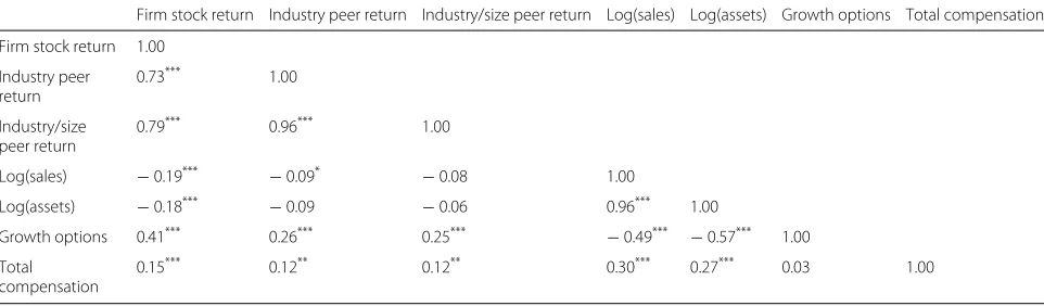
Table2shows Pearson correlation coefficients between

performance measures and the control variables firm size and growth options. Firm stock return and try peer return as well as firm stock return and indus-try/size peer return display positive correlations. The correlation of firm stock return with its industry peer return (0.73) is lower than the correlation of firm stock return with its industry/size peer return (0.79), which is consistent with previous evidence (Albuquerque 2009).18 The statistically significant correlation coeffi-cients increase our confidence that industry and indus-try/size peers are suited for filtering out noise from firm performance measures. In addition, total executive compensation is positively and significantly correlated with stock return (0.15). The same holds for the cor-relation between total compensation and industry peer return, and total compensation and industry/size peer return. Not surprisingly, total compensation is positively correlated with firm size. In order to identify a possi-ble multicollinearity propossi-blem in the upcoming regres-sions, we report variance inflation factors in all respective tables.19

3.3 Peer group composition

For the selection of the peer firm pool, we start with a comprehensive list of 4,228 firms, most of which are finan-cials. We use SIC-codes to remove firms which do not

belong to the banking industry.20We also exclude other

firms which we do not consider valid peers, such as the Allied Irish Banks, which technically became state-owned during the financial crisis. We then apply a number of screens to the return data to obtain a qualitatively sound data set (Ince and Porter2006). First, we delete any con-secutive zero returns at the end of the sample period.

Sec-ond, we remove returns below−80% and above 300%. We

also require that the one-year continuously compounded return obtained from monthly data is available. We end up with 1,570 firms as the pool of potential peers. Note that in order to mitigate survivorship bias, this pool also con-tains so-called “dead stocks” which were delisted from the stock market during the sample period.

RPE firms assess their CEOs’ compensation levels based on performance in relation to their respective peers. These peers are not simply a random draw of the mar-ket; firms follow a specific methodology in selecting their peers. Because researchers usually do not know a firm’s peers, a different approach is needed to approxi-mate the peer group. Most studies assessing RPE employ broad industry or market indices as a comparison group for peer performance. This is not without problems. Firms within an industry are hardly homogenous in their characteristics, so simple benchmarks are not able to adequately capture common shocks (Albuquerque 2009).21This introduces a bias in the statistical estimation and can distort inferences. An inappropriate compari-son group can lead to a higher (or lower) prescribed level of CEO pay. An expedient and replicable compari-son group based on a reacompari-sonable and objective criterion is therefore the key element when empirically testing for RPE.

Table 2Pearson correlation coefficients

Firm stock return Industry peer return Industry/size peer return Log(sales) Log(assets) Growth options Total compensation

Firm stock return 1.00

Industry peer return

0.73*** _1.00

Industry/size peer return

0.79*** 0.96*** 1.00

Log(sales) −0.19*** ₋_0.09* ₋_0.08 _1.00

Log(assets) −0.18*** ₋_0.09 ₋_0.06 _0.96*** _1.00

Growth options 0.41*** _0.26*** _0.25*** ₋_0.49*** ₋_0.57*** _1.00

Total compensation

0.15*** 0.12** 0.12** 0.30*** 0.27*** 0.03 1.00

(8)

Albuquerque (2009) provides a pragmatic solution for the ex post reconstruction of RPE peer groups. She com-poses groups based on both the two-digit SIC level and firm size. The first step in her process sorts firms by beginning-of-year market value into size quartiles within an industry. This yields four peer groups per industry. Each firm is then matched with its industry-size peer group. It turns out that this approach yields stronger empirical support for the use of RPE in executive com-pensation than sorting by industry classification alone, an improvement that is due to the information that firm size captures. Firms of comparable size are similar along several other characteristics which proxy for systematic risk. Albuquerque shows how the levels of diversifica-tion, financing constraints, and operating leverage vary with industry-size-ranked portfolios and provides evi-dence that firm size subsumes these characteristics. She finds that larger firms tend to be more diversified, have greater operating leverage, and smaller financing con-straints. This claim is supported by other literature. Dem-setz and Strahan (1997), for instance, construct a measure of diversification of BHCs. Their results establish a strong, positive effect of bank size on the diversification of BHCs. Moreover, small firms tend to face bigger financial con-straints in comparison to large ones. In other words, firm size is a proxy with high explanatory power for the

com-mon uncertainty Holmstrom (1982) insinuated. We thus

proceed to build the specific peer groups by adapting the

industry/size approach by Albuquerque (2009).

4 Results

4.1 Full sample results

This subsection presents the results for our full banking sample. We first present descriptive statistics of compensation data, performance measures, and firm

characteristics for the 46 firms during 2004–2013

(see the “Summary statistics” subsection). In the

“Regression results” section, we then document the sta-tistical results. We regress the logarithm of total CEO compensation on firm stock performance, peer return, and several control variables.

4.1.1 Summary statistics

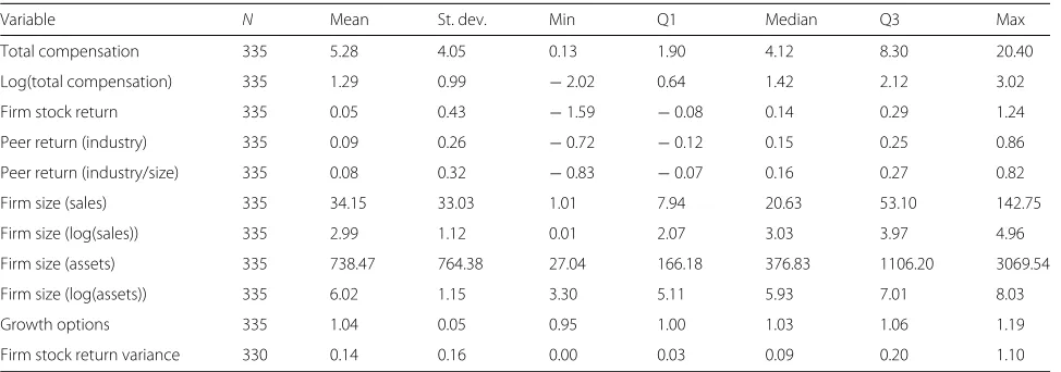
Table3presents descriptive statistics for the full sample. We report two measures of compensation: total compen-sation and the logarithm of total compencompen-sation. In the regression analysis, we use the logarithm of total com-pensation as a dependent variable because its empirical distribution is more symmetrical than the one for total compensation. This mitigates heteroscedasticity as well as extreme skewness and allows for a direct

compari-son with results from previous studies (Murphy 1999).

We also report summary statistics for the control vari-ables firm size (log of sales and sales) and growth options.

Table 3 shows that the average (median) total

compen-sation of an executive in our sample is USD 5.28 million (USD 4.12 million), which is not all that surprising in a sample that largely consists of major global players in the banking industry. Firm performance is measured using log-returns. The mean firm stock return is 5% and the median return is 14%. Averages of peer returns hover around 8%. The average (median) size in terms of sales of a bank is USD 34.15 billion (USD 20.63 billion). Using total assets as a proxy for size, the according value is USD 738.47 billion (USD 376.83 billion).

4.1.2 Regression results

We test the use of RPE in CEO compensation using Eq.1.

Peer groups are constructed with the industry and indus-try/size approach. We regress the logarithm of total CEO

Table 3Descriptive statistics

Variable N Mean St. dev. Min Q1 Median Q3 Max

Total compensation 335 5.28 4.05 0.13 1.90 4.12 8.30 20.40

Log(total compensation) 335 1.29 0.99 ₋2.02 0.64 1.42 2.12 3.02

Firm stock return 335 0.05 0.43 ₋1.59 ₋0.08 0.14 0.29 1.24

Peer return (industry) 335 0.09 0.26 ₋0.72 ₋0.12 0.15 0.25 0.86

Peer return (industry/size) 335 0.08 0.32 −0.83 −0.07 0.16 0.27 0.82

Firm size (sales) 335 34.15 33.03 1.01 7.94 20.63 53.10 142.75

Firm size (log(sales)) 335 2.99 1.12 0.01 2.07 3.03 3.97 4.96

Firm size (assets) 335 738.47 764.38 27.04 166.18 376.83 1106.20 3069.54

Firm size (log(assets)) 335 6.02 1.15 3.30 5.11 5.93 7.01 8.03

Growth options 335 1.04 0.05 0.95 1.00 1.03 1.06 1.19

Firm stock return variance 330 0.14 0.16 0.00 0.03 0.09 0.20 1.10

(9)

compensation on firm stock return, peer return, growth options, and log of sales. Year, country, and industry dummies are also included.

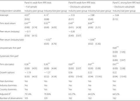
Panel A of Table4 shows the sensitivity of CEO total

compensation to RPE when using industry and indus-try/size peer groups. The coefficient on firm stock return is positive and statistically significant at the 1% level for both peer group specifications, with values of 0.47 and 0.55 for the industry and industry/size specifications, respectively. When the peer group is restricted to firms within the same industry, the coefficient of the peer port-folio is negative but not significant (−0.11 with apvalue of 0.56). Put differently, the performance of these peers does not seem to be filtered out from the CEO compen-sation contracts. If we include size into sorting and con-sider industry/size peers, the parameter estimates become

statistically significant (with a coefficient of−0.32 and ap value of 0.05). Robustness checks yield mixed results.22 23 By and large, the results for our international banks match previous findings for US firms, which showed that industry/size peers are better able to capture exogenous

shocks than industry peers alone (Albuquerque2009).

4.2 RPE subsample results 4.2.1 Weak tests of RPE

The results above are consistent with the notion that the 46 banks in our full sample follow an RPE scheme. We now turn to the informational value of peer disclo-sure. Although there is a risk of taking disclosure at face value, we exploit this information to sharpen our sam-ple’s profile. We test the sensitivity of CEO pay to RPE in the subsample of 25 banks that explicitly declare the use

Table 4Regressions estimating the sensitivity of CEO compensation to RPE

Panel A: weak-form RPE tests Panel B: weak-form RPE tests Panel C: strong-form RPE tests

– Full sample – Disclosure subsample – Disclosure subsample

Independent variables Industry peer group Industry/size peer group Industry peer group Industry/size peer group Industry/size peer group

Intercept 4.03** _4.13* ₋_3.55 ₋_2.88 ₋_5.64

(0.02) (0.08) (0.31) (0.40) (0.13)

Firm stock return 0.47*** _0.55*** _0.49** _0.69***

(0.00) [3.74] (0.00) [4.03] (0.01) [4.28] (0.00) [5.21]

Peer return (industry) −0.11 −0.30

(0.56) [4.15] (0.40) [5.07]

Peer return (industry/size) −0.32** ₋_0.66**

(0.05) [4.70] (0.02) [5.30]

Unsystematic firm perf 0.69***

(0.00) [1.85]

Systematic firm perf 0.03

(0.89) [2.87]

Firm size (sales) 0.36*** 0.36*** 0.69*** 0.67*** 0.67***

(0.00) [4.05] (0.00) [4.04] (0.00) [5.07] (0.00) [5.08] (0.00) [5.08]

Growth options ₋1.19 ₋1.27 0.56 0.22 0.22

(0.35) [4.53] (0.32) [4.54] (0.95) [13.43] (0.94) [13.45] (0.94) [13.45]

Year dummies Yes Yes Yes Yes Yes

Industry dummies Yes Yes Yes Yes Yes

Country dummies Yes Yes Yes Yes Yes

AdjustedR2 _79.14% _79.36% _63.27% _64.52% _64.52%

Number of observations 335 335 162 162 162

Note: Panels A and B show OLS regression results for the equationCompit=α0+α1·FirmPerfit+α2·PeerPerfit+α3·Cit+it. The first and third column show the results

from regressing log of total CEO compensation on stock return, peer performance composed of the firms within the same industry, and control variables. The second and fourth column document regression results based on the industry/size quartiles peer group approach by Albuquerque (2009). Panel A shows the results for the full sample, and panel B reports the results for the disclosure subsample. Panel C documents OLS regression results for the equationCompit=δ0+δ1·UnsysFirmPerformanceit

+δ2·SystFirmPerformanceit+δ3·Cit+eiton the subsample of disclosing banks. We regress the logarithm of CEO compensation on the unsystematic firm performance,

(10)

of peers in determining the performance of their CEOs

in their statement proxies (see the “Compensation data”

section). We follow the same empirical specification used in the previous analysis.

Panel B of Table 4 shows the sensitivity of CEO total

compensation to RPE when using industry and indus-try/size peers. The results show positive and statistically significant parameter estimates on firm stock perfor-mance for both peer group specifications. The estimates are 0.49 and 0.69, respectively, indicating that a CEO is being rewarded for positive firm performance. Hence, on average, CEO compensation increases with firm perfor-mance. When the peer groups are composed of banks within the same industry, the coefficient on the peer port-folio is negative and not significant (with a coefficient of

−0.30 and apvalue of 0.40). The industry/size

parame-ter estimate is also negative but statistically significant at the 5% level (with a coefficient of−0.66 and apvalue of 0.02). The results for the subsample of disclosing banks, too, provide evidence consistent with RPE, but more con-clusively so than the results for the full sample. The coef-ficient on the peer portfolio doubles in size and increases in statistical significance.24This suggests that peer group disclosure holds informational value regarding RPE. One could also say that the inclusion of non-disclosing banks in the full sample tends to dilute the statistical inference and renders it less conclusive.25These results stand in contrast to Gong et al. (2011), who find no informational value of RPE disclosure. However, their sample only comprises US firms for 1 year.

4.2.2 Strong-form test of RPE

Following Antle and Smith (1986), we perform so-called

strong-form tests of RPE on the subsample of RPE disclo-sures to verify the robustness of our results. Strong-form tests of RPE examine whether all the noise that can be removed is indeed filtered out from the compensation contracts. Details on the construction of systematic and unsystematic firm performances and the employed

empir-ical model are reported in the “Empirical model”

subsec-tion. In a nutshell, the results are consistent with RPE if only the unsystematic performance exerts influence on CEO pay, and not the systematic one.

Panel C of Table 4 documents the regression results

from Eq. (4) for the subsample of disclosing banks. Here, we regress the logarithm of CEO compensation on unsys-tematic firm performance, sysunsys-tematic firm performance, and control variables for 162 firm-year observations over the time span 2004–2013. In that specification, we restrict ourselves to industry/size groups for constructing the sys-tematic performance variable. The syssys-tematic component

is not significant with a coefficient estimate of 0.03 (p

value = 0.89). The unsystematic performance variable, on the other hand, is positive and statistically significant with

a coefficient of 0.69 (pvalue = 0.00). This suggests that the CEOs in our subsample are being compensated for unsys-tematic performance only. These results hold up to several robustness tests and provide evidence in keeping with the use of strong-form RPE and reinforce the previous find-ing that CEOs are not befind-ing compensated for systematic

performance in the subsample of RPE disclosures.26

5 Extensions and robustness checks

5.1 Associated factors of RPE in the banking industry

Prior studies have put forth a variety of factors that are related to the usage of RPE in compensation contracts in

UK and US firms (Carter et al. 2009; Gong et al.2011;

Albuquerque 2014). They do not, however, examine the

relation of one factor at a time on the usage of RPE while controlling for other factors. Gong et al. (2011) investigate explicit disclosures on RPE in the US to identify the fac-tors that prompt the use of RPE in compensation contracts

in 2006. Carter et al. (2009) examine the use of RPE in

performance-vested equity grants in a sample of UK firms in 2002. This section examines international firms over a longer time span. Understanding what factors are linked to RPE is instructive for researchers testing for RPE and could offer yet another reason for the mixed evidence in existing empirical studies.

In order to pinpoint possible factors related to RPE, we

conduct a logit regression. The dependent variableyit is

an indicator variable that equals 1 for banks that disclose information on the use of a peer group to determine the level of executive compensation, and 0 otherwise

(see the “Compensation data” section). The independent

variables include CEO pay (Comp_it), firm performance

(FirmPerf_it), various specifications of peer return (PeerPerf_it), and control variables. We control for firm size (FirmSizeit) and growth options (GrowthOptionsit)

and include year (YearDummy_it), industry

(IndustryDummy_it), and country (CountryDummy_it) dummies to control for cross-sectional variation. Sales are used as a proxy for firm size. Growth

options are calculated as follows: (Market Equity+

Total Assets−Common Equity)/Total Assets.

Our logit model is based on the following latent variable model:

yit=γ0+γ1·Compit+γ2·FirmPerfit +γ3·PeerPerfit+γ4·FirmSizeit

+γ5·GrowthOptionsit+γ7·YearDummyit +γ8·IndustryDummyit

+γ9·CountryDummyit+uit. (5)

We estimate Eq. (5) with the full sample of 335

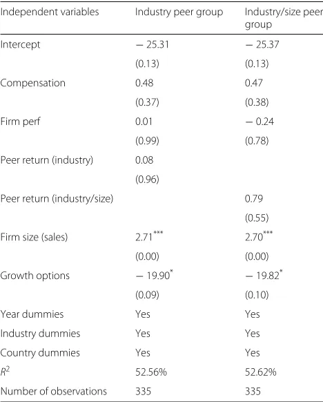
firm-year observations from 2004 to 2013. Table5reports the

(11)

Table 5Logit regression of RPE usage in executive compensation contracts

Independent variables Industry peer group Industry/size peer group

Intercept ₋25.31 ₋25.37

(0.13) (0.13)

Compensation 0.48 0.47

(0.37) (0.38)

Firm perf 0.01 −0.24

(0.99) (0.78)

Peer return (industry) 0.08

(0.96)

Peer return (industry/size) 0.79

(0.55)

Firm size (sales) 2.71*** 2.70***

(0.00) (0.00)

Growth options ₋19.90* ₋_19.82*

(0.09) (0.10)

Year dummies Yes Yes

Industry dummies Yes Yes

Country dummies Yes Yes

R2 _52.56% _52.62%

Number of observations 335 335

Note: This Table documents logit regression results for the equation

yit=γ0+γ1·Compit+γ2·FirmPerfit+γ3·PeerPerfit+γ4·Cit+uit. The

dependent variable isRPE, an indicator variable which is equal to 1 if the firm discloses peer group use in the compensation contracts. We regressRPEon firm performance, peer returns, firm size, and growth options for 335 firm-year observations over the time span 2004–2013. We also include year, country, and industry dummies in the regression estimation for two specifications, industry and industry/size peers. We report Cox and Snell’sR2_{and model coefficient estimates.} Significance levels are denoted as follows: 1% (∗ ∗ ∗), 5% (∗∗), and 10% (∗). The correspondingpvalues are reported in parentheses below each coefficient estimate

options for industry and industry/size peers.27_The

oppo-site holds for growth options.28 _{None of the other}

pre-dictors are statistically significant, indicating that in our sample there is a strong link between size and growth

options on the one hand and RPE on the other one.29

These results are in line with existing evidence. Gong et al. (2011) find that larger firms are more likely to use RPE. This could be for several reasons. Firm size might represent a crude proxy for public scrutiny and share-holder concerns about compensation practices. Larger firms are also more exposed to monitoring pressure compared to smaller firms. This might well force them to be more committed to RPE (Bannister and Newman

2003). Albuquerque (2014) and Gong et al. (2011) find

that the level of RPE in CEO compensation contracts is negatively associated with a firm’s level of growth options.

Carter et al. (2009) examine the disclosure of

performance-based conditions in equity grants and document that growth options are inversely related

to the performance-based conditions. Albuquerque

(2014) argues that high growth options firms have to

bear more risks and thus exhibit a higher idiosyncratic variance. These firms are also characterized by firm-specific know-how and operate in markets with high barriers to entry. As a consequence, these characteristics make peer performance uninformative with respect to capturing external shocks. This eventually leads to less usage of RPE among high growth options firms (Albuquerque,2014, p.1).

5.2 RPE pay practices and bank-level characteristics

We next extend our analysis and investigate the relation between the magnitude of RPE pay practices and various bank-level characteristics. We first repeat the standard estimation (Eq.1) conducted in the “Regression results” section with the industry/size peer group. We quan-tify RPE-intensity via the ratio of predicted (log) CEO-compensation to the actual (log) CEO-CEO-compensation. This prediction is only based on firm stock return and peer group return. The idea here is to separate firms (or firm-years) for which compensation is mainly based on firm performance and peer group performance from firms (or firm-years) for which other factors are more impor-tant. We then proceed to sort all firm-years based on this measure of RPE-intensity into four groups of equal size to examine if various bank-level characteristics are related to RPE-intensity. We analyze three different measures; two proxies for firm performance and one proxy for firm-specific risk: (1) return on equity (ROE), (2) the (yearly) firm stock return, and (3) the variance of the firm stock return. We calculate ROE by dividing net sales (Datas-tream code DWSL) by lagged common equity (World-scope item WC03501). The calculation of the yearly stock return is described in the “International banking sample” section. Finally, firm stock return variance is calculated as the variance of the stock returns over the previous 36 months.

The results are shown in Table6. Between RPE-intensity

(12)

Table 6RPE pay practices and bank-level characteristics RPE-intensity

group

N ROE Firm stock return Firm stock return variance

1 83 1.21 0.05 0.16

(0.48) (0.42) (0.16)

2 84 1.13 0.12 0.13

(0.51) (0.30) (0.17)

3 84 1.04 0.07 0.12

(0.60) (0.40) (0.12)

4 84 1.24 -0.02 0.17

(0.65) (0.56) (0.19)

Note: Using RPE-intensity, we classify firm-year observations into four groups. RPE-intensity is calculated as the ratio of predicted (log) CEO compensation to actual (log) CEO compensation. The ratio of predicted to actual CEO compensation is lowest in group 1 and highest in group 4. ROE is calculated by dividing net sales (datastream code DWSL) by lagged common equity (worldscope item WC03501). The calculation of the yearly stock return is based on the yearly total return index by datastream based on the respective fiscal year. Firm stock return variance is calculated as the variance of the stock returns over the previous 36 months. The table reports group means for each measure. Standard deviations are shown in parentheses

5.3 Robustness checks

In this section, we conduct three different checks to gauge

the robustness of the results obtained in the “Results”

section: (1) we construct regional instead of global peer groups, (2) we construct value-weighted instead of equal-weighted peer groups, and (3) we examine the effect of excluding the years of the financial crisis (2007 and 2008).

5.3.1 Regional peer groups

Our first robustness check restricts the construction of the peer group by employing regional instead of global peer groups. We first classify seven regions as

defined by the World Bank:30 “Europe and Central

Asia," "Middle East and North Africa," "Latin America and Caribbean," "East Asia and Pacific,” “South Asia,”

“Sub-Saharan Africa,” and “North America.” Not surpris-ingly, the correlations between peer and firm stock returns are somewhat higher with regional peer groups than with

global peer groups (as shown in Tables7 and2,

respec-tively). The correlation between industry peer group and total compensation is no longer significant. The correla-tion between industry/size peer group and total compen-sation, on the other hand, does not change from going regional.

Table 8 replicates the main results of the

“Regression results” section using regional peer groups. By and large, the results are similar to the ones obtained

with global peer groups in the “Regression results”

section. The coefficients of the industry/size peer group remain significant at the 5% level for both the full sample and the disclosure subsample. The strong-form RPE test for the disclosure subsample continues to support the hypothesis that firms apply RPE.

5.3.2 Value-weighted peer groups

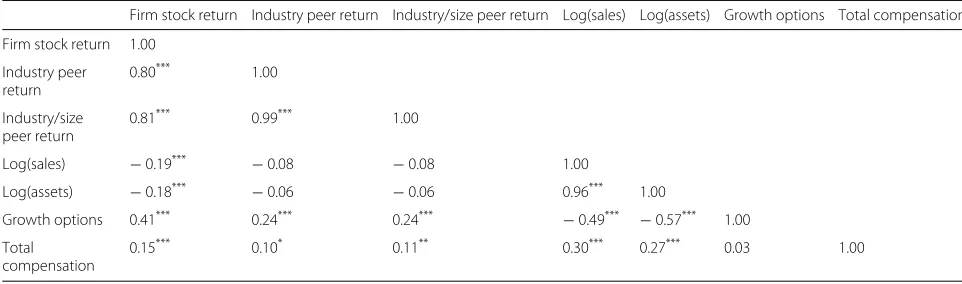
With a skewed distribution, equal weights might over-state the influence of smaller banks in peer groups. This is a concern in our sample because it contains the largest banks in the world, possibly biasing our results. To mit-igate the impact of smaller banks, the next robustness check employs value-weighted instead of equal-weighted peer groups. For this purpose, we use the market capital-ization at the fiscal year date. Table9shows the according correlations. The results do not change much compared

to equal-weighted peer groups as shown in Table2.

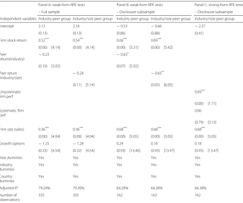
Table 10 replicates the main results of the

“Regression results” section using value-weighted peer groups. The differences between the industry and the industry/size peer groups become less pronounced. This is to be expected because value weights shift the focus to the biggest firms in each industry, and the banks in our sample are most likely in this group. Taken together, we come to the same conclusions: the size/industry

Table 7Pearson correlation coefficients with regional peer groups

0.80*** _1.00

0.85*** 0.93*** 1.00

Log(sales) −0.19*** ₋_0.12** ₋_0.13** _1.00

Log(assets) −0.18*** ₋_0.13** ₋_0.12** _0.96*** _1.00

Growth options 0.41*** _0.30*** _0.30*** ₋_0.49*** ₋_0.57*** _1.00

Total compensation

0.15*** _0.07 _0.12** _0.30*** _0.27*** _0.03 _1.00

(13)

Table 8Regressions estimating the sensitivity of CEO compensation to RPE with regional peer groups

Intercept 2.08** _2.25* ₋_0.84 ₋_0.60 ₋_2.44

(0.02) (0.08) (0.78) (0.84) (0.42)

(0.00) [4.39] (0.00) [4.68] (0.02) [6.17] (0.00) [7.22]

Peer

return(industry) −

0.09 −0.29

(0.59) [4.58] (0.37) [5.99]

Peer return

(industry/size) −

0.31** ₋_0.66**

(0.04) [5.46] (0.02) [6.97]

Unsystematic firm perf

0.85***

(0.00) [1.69]

Systematic firm perf

0.09

(0.63) [2.72]

Firm size (sales) 0.36*** _0.36*** _0.70*** _0.65*** _0.65***

(0.00) [4.04] (0.00) [4.05] (0.00) [5.03] (0.00) [5.17] (0.00) [5.17]

Growth options −1.12 −1.37 0.48 0.33 0.33

(0.34) [4.57] (0.28) [4.56] (0.87) [13.48] (0.90) [13.42] (0.90) [13.42]

Industry dummies

Yes Yes Yes Yes Yes

Country dummies

Yes Yes Yes Yes Yes

AdjustedR2 _79.14% _79.42% _63.28% _64.92% _64.92%

Number of observations

335 335 162 162 162

Note: PanelS A and B show OLS regression results for the equationCompit=α0+α1·FirmPerfit+α2·PeerPerfit+α3·Cit+it. The first and third columns show the results

from regressing log of total CEO compensation on stock return, peer performance composed of the firms within the same industry, and control variables. The second and fourth columns document regression results based on the industry/size quartiles peer group approach by Albuquerque (2009). Panel A shows the results for the full sample, and panel B reports the results for the disclosure subsample. Panel C documents OLS regression results for the equationCompit=δ0+δ1·UnsysFirmPerformanceit

+δ2·SystFirmPerformanceit+δ3·Cit+eiton the subsample of disclosing banks. We regress logarithm of CEO compensation on the unsystematic firm performance,

systematic firm performance, and control variables for 162 firm-year observations over the time span 2004–2013. We use industry/size peer group specification in order to construct a systematic performance variable. All regressions include year, industry, and country dummies. For more details on systematic and unsystematic variable construction see the “Empirical model” section. Peer groups are constructed for seven different regions. Significance levels are two-sided and denoted as follows: 1% (∗ ∗ ∗), 5% (∗∗), and 10% (∗). The correspondingpvalues are reported in parentheses below each coefficient estimate. Variance inflation factors are reported in squared brackets

peer group still performs better than the industry peer group, and the strong-form RPE test for the disclosure subsample continues to support the hypothesis that firms apply RPE.

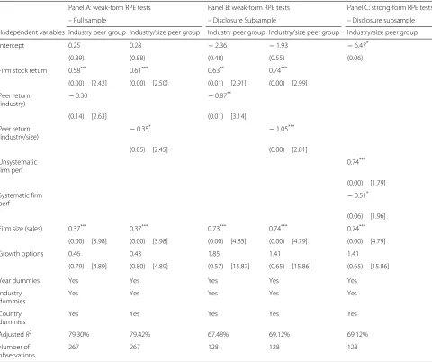
5.3.3 Exclusion of financial crisis years

The financial crisis in 2007 and 2008 had far-reaching implications for the performance of banks

(e.g., Fahlenbrach and Stulz (2011)). These crisis years

might distort the results of our analysis by driving the

correlation between firm performance and industry/size peer return. In a third robustness check, we exclude the

years 2007 and 2008 from our sample.31

The correlations obtained without the years 2007 and

2008 strongly differ from the baseline results in Table2

(14)

Table 9Pearson correlation coefficients with value-weighted peer groups

0.80*** _1.00

0.81*** 0.99*** 1.00

Log(sales) −0.19*** ₋_0.08 ₋_0.08 _1.00

Log(assets) −0.18*** ₋_0.06 ₋_0.06 _0.96*** _1.00

Growth options 0.41*** _0.24*** _0.24*** ₋_0.49*** ₋_0.57*** _1.00

Total compensation

0.15*** _0.10* _0.11** _0.30*** _0.27*** _0.03 _1.00

Note: This table shows Pearson product moment correlation coefficients between total compensation, performance measures, and control variables. Peer groups are constructed using value weights. The sample consists of 335 observations covering the time period 2004–2013. Significance levels are denoted as follows: 1% (***), 5% (**), and 10% (*)

We next examine whether this substantial change in correlations affect the main conclusions from our

base-line results. Table 11 shows that the peer group

coef-ficients become generally more negative. But the weak-form regression paints the same picture as the baseline results: Size/industry peer groups have larger coefficients than industry-only peer groups, and the disclosure sub-sample shows stronger evidence in favor of RPE than the full sample. The strong-form regressions reject the hypothesis that systematic risk is not filtered out of the compensation contract at a 5% level of statistical signifi-cance (instead of 10% in the other results).

5.3.4 Additional robustness checks

We performed additional, unreported robustness

checks.32 Using total assets instead of sales as a proxy

for firm size yields very similar results. Value-weighted regional peer groups do not substantially alter the results of the baseline specification, either. Finally, in order to disentangle cross-sectional from time-series effects, we conduct a panel estimation with fixed year-effects and fixed bank-effects. The between-group estimates yield mostly insignificant coefficients. The coefficient for the disclosure subsample with the size/industry peer group, however, is negative and significant (at the 5% level), and thus in line with our baseline result.

6 Conclusion

This papers tests the presence of RPE in an original sample of 46 international banks from 2004 to 2013. We regress the logarithm of total compensation on firm performance, industry and industry/size peer performance, and control variables such as firm size and growth options. We control for unobservable variation in the level of compensation across years, industries, and countries. When we account for peer groups with peer selection based on industry and firm size, we find evidence for the use of RPE in

international banking. This evidence becomes stronger once we focus on banks who openly disclose the use of peers in their remuneration practice. This insight contrasts and complements previous findings for the US.

We next employ a logit regression model to identify fac-tors related to RPE in international banking. The evidence supports the working theory that growth options and firm size play a crucial role in banks’ decisions to use RPE. Our results are robust to different model specifications and are consistent with existing evidence. We find that the likeli-hood of RPE usage is decreasing with growth options. A possible explanation for this result is that the implemen-tation of RPE in high growth option banks might be too costly due to difficulties in identifying the correct peer group, rendering such banks less likely to use RPE. We also find that larger banks are more inclined to use RPE in their compensation contracts. This is a plausible finding. In light of the recent financial crisis, high levels of CEO com-pensation have attracted a lot of attention, and large banks in particular have been under significant monitoring and shareholder pressure. In response to such pressure, large banks are more likely to have become incentivized to be committed to RPE usage in determining the level of CEO pay.

(15)

Table 10Regressions estimating the sensitivity of CEO compensation to RPE with value-weighted peer groups

Intercept 2.12 2.16 ₋0.53 ₋0.46 ₋2.57

(0.13) (0.13) (0.86) (0.88) (0.41)

Firm stock return 0.52*** _0.54*** _0.66*** _0.69***

(0.00) [4.14] (0.00) [4.14] (0.00) [5.31] (0.00) [5.42]

Peer

return(industry) −

0.23 −0.63*

(0.19) [5.05] (0.07) [5.92]

Peer return

(industry/size) −

0.28 ₋0.65**

(0.11) [5.14] (0.05) [6.05]

0.69***

(0.00) [1.71]

Systematic firm perf

0.06

(0.79) [3.15]

Firm size (sales) 0.36*** _0.36*** _0.68*** _0.68*** _0.68***

(0.00) [4.04] (0.00) [4.04] (0.00) [5.05] (0.00) [5.05] (0.00) [5.05]

Growth options −1.25 −1.28 0.24 0.18 0.18

(0.33) [4.54] (0.32) [4.54] (0.93) [13.46] (0.95) [13.47] (0.95) [13.47]

Industry dummies

Yes Yes Yes Yes Yes

Country dummies

Yes Yes Yes Yes Yes

AdjustedR2 _79.24% _79.30% _64.20% _64.38% _64.38%

335 335 162 162 162

Note: Panels A and B show OLS regression results for the equationCompit=α0+α1·FirmPerfit+α2·PeerPerfit+α3·Cit+it. The first and third column show the results

+δ2·SystFirmPerformanceit+δ3·Cit+eiton the subsample of disclosing banks. We regress logarithm of CEO compensation on the unsystematic firm performance,

systematic firm performance, and control variables for 162 firm-year observations over the time span 2004–2013. We use industry/size peer group specification in order to construct a systematic performance variable. All regressions include year, industry, and country dummies. For more details on systematic and unsystematic variable construction, see the “Empirical model” section. Peer groups are constructed with value weights. Significance levels are two-sided and denoted as follows: 1% (∗ ∗ ∗), 5% (∗∗), and 10% (∗). The correspondingpvalues are reported in parentheses below each coefficient estimate. Variance inflation factors are reported in squared brackets

their own, CEOs would rather follow their own ways to maximize utility. RPE helps align the interest of share-holders and CEOs by creating incentives for CEOs to take actions to increase shareholder wealth. Third, in line with previous studies, our evidence indicates that industry/size peers are better able to capture exogenous shocks than industry peers alone. Finally, empirical evidence on RPE runs the risk of diluting. In studies of RPE, it seems, if nothing else for robustness, to stratify empirical samples by disclosure. This should inform future research.

Endnotes

1_{Implementing RPE does also entail potential costs.}

(Gibbons and Murphy 1990, p. 31) discuss the benefits

(16)

externali-Table 11Regressions estimating the sensitivity of CEO compensation to RPE without the years 2007 and 2008

– Full sample – Disclosure Subsample – Disclosure subsample

Intercept 0.25 0.28 ₋2.36 ₋1.93 ₋6.47*

(0.89) (0.88) (0.48) (0.55) (0.06)

(0.00) [2.42] (0.00) [2.50] (0.01) [2.91] (0.00) [2.99]

Peer return

(industry) −

0.30 −0.87**

(0.14) [2.63] (0.01) [3.14]

Peer return

(industry/size) −

0.35* ₋_1.05***

(0.05) [2.45] (0.00) [2.81]

0.74***

(0.00) [1.79]

Systematic firm

perf −

0.51*

(0.06) [1.96]

Firm size (sales) 0.37*** _0.37*** _0.73*** _0.74*** _0.74***

(0.00) [3.98] (0.00) [3.98] (0.00) [4.85] (0.00) [4.79] (0.00) [4.79]

Growth options 0.46 0.43 1.85 1.41 1.41

(0.79) [4.89] (0.80) [4.89] (0.57) [15.87] (0.65) [15.86] (0.65) [15.86]

Industry dummies

Yes Yes Yes Yes Yes

Country dummies

Yes Yes Yes Yes Yes

AdjustedR2 _79.30% _79.42% _67.48% _69.12% _69.12%

267 267 128 128 128

Note: Panels A and B show OLS regression results for the equationCompit=α0+α1·FirmPerfit+α2·PeerPerfit+α3·Cit+it. The first and third columns show the results

+δ2·SystFirmPerformanceit+δ3·Cit+eiton the subsample of disclosing banks. We regress logarithm of CEO compensation on the unsystematic firm performance, systematic

firm performance, and control variables for 128 firm-year observations over the time span 2004–2006 and 2009–2013. We use industry/size peer group specification in order to construct a systematic performance variable. All regressions include year, industry, and country dummies. For more details on systematic and unsystematic variable construction, see the “Empirical model” section. Peer groups are constructed for seven different regions. Significance levels are two-sided and denoted as follows: 1% (∗ ∗ ∗), 5% (∗∗), and 10% (∗). The correspondingpvalues are reported in parentheses below each coefficient estimate. Variance inflation factors are reported in squared brackets

ties), they find that most of the costs are of minor rele-vance for CEO compensation (for details see Gibbons and

Murphy1990).

2_{This is known as Bebchuck and Fried’s (2004)}

man-agerial power hypothesis, which argues that there are serious flaws in the corporate governance system, flaws that allow executives to exert influence over the board of the directors and thereby hold sway over the level of their pay. Bebchuck and Fried provide evidence that

supports their hypothesis, which helps explain why the actual pay-setting process is hard to reconcile with tradi-tional contract theory.

3_{Antle and Smith (}₁₉₈₆_{) examine RPE in a sample of}

chemical, aerospace, and electronics firms. Rajgopal et al.

(2006) cover a wide range of industries with the three

largest groups being electric, gas, and sanitary services, chemicals and allied products, and depository