Non-Parallel Training in Voice Conversion
Using an Adaptive Restricted Boltzmann Machine
著者(英)
Toru Nakashika, Tetsuya Takiguchi, Yasuhiro
Minami
journal or
publication title
IEEE/ACM Transactions on Audio, Speech, and
Language Processing
volume
24
number
11
page range
2032-2045
year
2016-11
URL
http://id.nii.ac.jp/1438/00008972/
doi: 10.1109/TASLP.2016.2593263Non-Parallel Training in Voice Conversion Using an
Adaptive Restricted Boltzmann Machine
Toru Nakashika,
Member, IEEE,
, Tetsuya Takiguchi,
Member, IEEE
and Yasuhiro Minami,
Member, IEEE
Abstract—In this paper, we present a voice conversion (VC) method that does not use any parallel data while training the model. VC is a technique where only speaker specific information in source speech is converted while keeping the phonological information unchanged. Most of the existing VC methods rely on parallel data—pairs of speech data from the source and target speakers uttering the same sentences. However, the use of parallel data in training causes several problems; 1) the data used for the training is limited to the pre-defined sentences, 2) the trained model is only applied to the speaker pair used in the training, and 3) mismatches in alignment may occur. Although it is, thus, fairy preferable in VC not to use parallel data, a non-parallel approach is considered difficult to learn. In our approach, we achieve non-parallel training based on a speaker adaptation technique and capturing latent phonological information. This approach assumes that speech signals are produced from a RBM(restricted Boltzmann machine)-based probabilistic model, where phonological information and speaker-related information are defined explicitly. Speaker-independent (SI) and speaker-dependent (SD) parameters are simultaneously trained under speaker adaptive training. In the conversion stage, a given speech signal is decomposed into phonological and speaker-related information, the speaker-speaker-related information is replaced with that of the desired speaker, and then voice-converted speech is obtained by mixing the two. Our experimental results showed that our approach outperformed another non-parallel approach, and produced results similar to those of the popular conventional GMM-based method that used parallel data in subjective and objective criteria.
Index Terms—Voice conversion, restricted Boltzmann machine, unsupervised training, speaker adaptation.
I. INTRODUCTION
I
N recent years, voice conversion (VC), which is a technique used to change speaker-specific information in the speech of a source speaker into that of a target speaker while retaining linguistic information, has been garnering much attention since the VC techniques can be applied to various tasks [1], [2], [3], [4], [5]. Most of the existing approaches rely on statistical models [6], [7], and the approaches based on Gaussian mixture models (GMM) [8], [9], [10], [11] are one of the mainstream methods nowadays. Other statistical models, such as non-negative matrix factorization (NMF) [12], [13], neural networks (NNs) [14], restricted Boltzmann machines (RBMs) [15], [16], and deep learning [17], [18], are also used in VC. However, almost all of the existing VC methods require T. Nakashika and Y. Minami are with the Graduate School of Informa-tion Systems, University of Electro-CommunicaInforma-tions, Tokyo, Japan e-mail: [email protected], [email protected]T. Takiguchi is with Organization of Advanced Science and Technol-ogy, Kobe University, 1-1 Rokkodai, Nada, Kobe 657-8501, Japan e-mail: [email protected]
Manuscript received April 19, 2005; revised December 27, 2012.
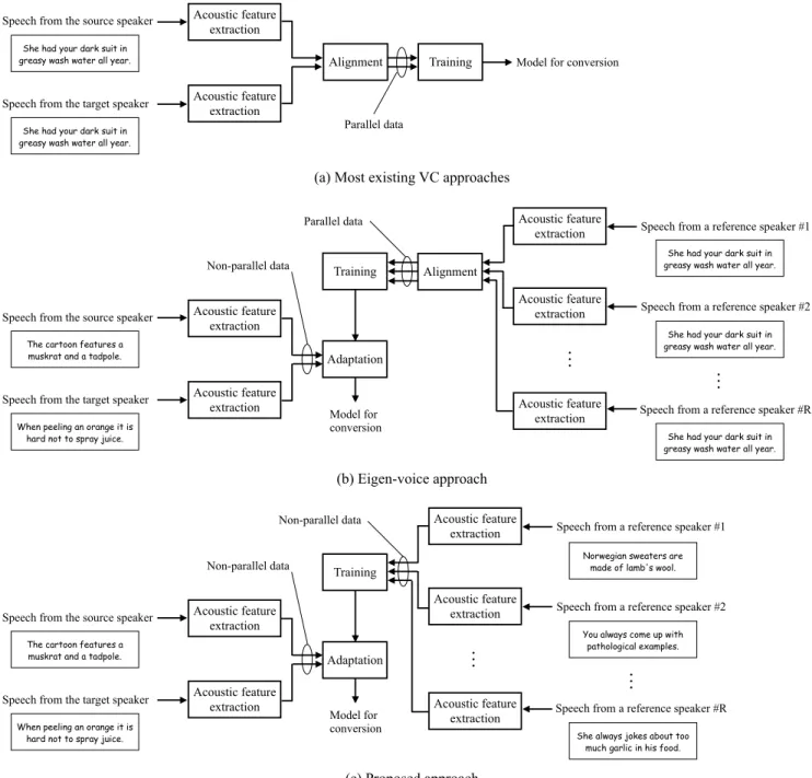
parallel data (speech data from the source and the target speakers aligned so that each frame of the source speaker’s data corresponds to that of the target speaker) for training the models, as shown in Fig. 1 (a), which leads to several problems. First, the transcriptions of the training data must be the same for both speakers, which means that the training data should be pre-defined and is considerably limited. Second, the trained model is only applied to the speaker pair used in the training, and it is difficult to reuse the model on the conversion of another speaker pair. Third, the training data (the parallel data) is not the original speech data anymore because the speech data is stretched and modified in the time axis when aligned. Furthermore, it is not guaranteed that each frame is aligned perfectly, and mismatching may cause some errors in training.
Several approaches that do not use parallel data from the source to the target speakers have been also proposed [19], [20], [21], [22]. In [19]; for example, they model the spec-tral relationships between two arbitrary speakers (reference speakers) using GMMs, and convert the source speaker’s speech using the matrix that projects the feature space of the source speaker into that of the target speaker through that of reference speakers. As a result, parallel data from the source and target speakers is not required. In [21], codebooks (eigenvoice) are obtained using the parallel data of reference speakers, and many-to-many VC is achieved by mapping the source speaker’s speech into eigenvoice and the eigenvoice into the target speaker’s speech. However, these approaches still require parallel data among reference speakers (Fig. 1 (b)), which causes the above-mentioned problems (regarding the limitation of the corpus used in training) to remain.
In this paper, we tackle a totally-parallel-data-free1 VC
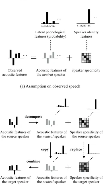
method that uses a model on latent phonological information that produces neutral speech, along with a speaker adaptation technique. The idea behind this is simple and intuitive. As shown in Fig. 2 (a), we assume that observed acoustic features obtained from an arbitrary speaker’s speech are considered to be composed of the neutral acoustic feature that is linked with the phonological information (the probability of latent phonological features) and belongs to no one, accompanied with the speaker specificity that is linked with the speaker-related information (speaker identity features)2. In this as-1This means that the method requires neither the parallel data of a source
speaker and target speaker, nor the parallel data of reference speakers as shown in Fig. 1 (c).
2We use the term “features” for phonological information and
speaker-related information, since they are also used as inputs when generating speech signals.
(a) Most existing VC approaches
(c) Proposed approach (b) Eigen-voice approach She had your dark suit in
greasy wash water all year.
Speech from the source speaker
Speech from the target speaker
She had your dark suit in greasy wash water all year.
Acoustic feature extraction
Alignment Training
Parallel data
Model for conversion
The cartoon features a muskrat and a tadpole.
Speech from the source speaker
Speech from the target speaker
When peeling an orange it is hard not to spray juice.
Norwegian sweaters are made of lamb's wool.
Speech from a reference speaker #1
Speech from a reference speaker #2
You always come up with pathological examples.
…
Speech from a reference speaker #R
She always jokes about too much garlic in his food.
…
Non-parallel data
Non-parallel data
The cartoon features a muskrat and a tadpole.
Speech from the source speaker
Speech from the target speaker
When peeling an orange it is hard not to spray juice.
Non-parallel data
Speech from a reference speaker #1
Speech from a reference speaker #2
…
Speech from a reference speaker #R
…
Parallel data
She had your dark suit in greasy wash water all year.
She had your dark suit in greasy wash water all year.
She had your dark suit in greasy wash water all year.
Model for conversion Acoustic feature extraction Acoustic feature extraction Acoustic feature extraction Alignment Acoustic feature extraction Training Adaptation Acoustic feature extraction Acoustic feature extraction Acoustic feature extraction Acoustic feature extraction Model for conversion Training Adaptation Acoustic feature extraction Acoustic feature extraction Acoustic feature extraction
Fig. 1: Comparison of training schemes in each VC approach. sumption, VC is achieved by three steps: decomposing a
speech signal into neutral speech and speaker specific in-formation, replacing the speaker specific information with that of the desired speaker, and composing a speech signal using the neutral speech and the speaker information that was replaced (Fig. 2 (b)). The proposed probabilistic model, called an adaptive restricted Boltzmann machine (ARBM), is designed to help such decomposition. The model is an energy-based function like a restricted Boltzmann machine (RBM), and consists of a visible layer and a hidden layer having undirected connections between visible-hidden units with the weights of the connections that vary with the speaker. The weights are defined as a sum-product of speaker-independent and speaker-dependent weight matrices, and these weights can
be simultaneously optimized so as to maximize the likelihood of speech data that contains multiple speakers (not required to be parallel data). Most of the related work in VC focuses not on F0 conversion but on the conversion of spectrum features, and we conform to that in this paper as well.
Another advantage of the proposed method is that it al-lows many-to-many voice conversion. Once speaker specific features of a certain speaker are obtained, the speaker can be used as a source speaker to any other speakers, and as a target speaker from any other speakers.
This paper is organized as follows. The definition and the parameter optimization of the ARBM are presented in section II. In section III, the way in which we applied the ARBM to VC is described. We give the VC experimental results in
Observed acoustic features
=
+
/sh//i/ /k/…
/m/ Speaker specificity Acoustic features ofthe neutral speaker
Acoustic features of the source speaker
+
Speaker specificity of the source speaker Acoustic features of
the neutral speaker Latent phonological features (probability)
+
Acoustic features of
the target speaker Acoustic features of the neutral speaker Speaker specificity of the target speaker
decompose
combine
copy replace
(b) Voice-conversion scheme in proposed method (a) Assumption on observed speech
#2#3 #4
…
#1 Speaker identity features…
…
Fig. 2: The idea of voice conversion without using parallel data in training. In the conversion stage, only the speaker specific features are changed while keeping the phonological informa-tion that is linked with the neutral speaker’s acoustic features. The symbol “+” indicates combinationfor convenience, and does not indicate a plus operator here.
section IV, and conclude the paper in section V.
II. ADAPTIVE RESTRICTEDBOLTZMANN MACHINE A. Definition
In our speech modeling assumption, observed acoustic features are represented by two factors: latent phonological information and speaker specific features. The unobservable phonological information is not speaker-dependent and may produce the neutral acoustic features that exclude speaker specificity. On the other hand, the speaker-specific features rely upon the speaker.
Restricted Boltzmann machine(RBM [23], [24])-based probabilistic models are convenient for representing such
v
h ¯ W s AFig. 3: Graphical representation of an ARBM.
latent features that are cannot be observed but surely exist in the background. As an extension of RBMs, in order to extract speaker specific features, we define a probabilistic model called an “adaptive restricted Boltzmann machine” (ARBM) as shown in Figure 3. In this model, we represent observed acoustic features and latent phonological features as the visible units v ∈ RI and hidden units h ∈ {0,1}J,
respectively (I and J indicate the numbers of dimensions in acoustic features and latent phonemes, respectively). In addition to visible units and hidden units, we introduce speaker identity unitss∈ {0,1}R,PR
r=1sr= 1that represent which
speaker utters the sentence (Ris the number of speakers used in the training). Usually s is used as a one-hot vector. For example, if we have one-hot vector s, whose elements are sr = 1,∀sr0 = 0 (r0 6= r), it means that the rth speaker
is of interest. In this model, the connection weights between visible units and hidden units and bias terms of the visible units and the hidden units are controlled by s. We define the visible-hidden connectionsW(s), the visible biases b(s)and the hidden biasesc(s)as follows:
W(s) =X r ArsrW¯ (1) b(s) = ¯b+X r brsr= ¯b+Bs (2) c(s) = ¯c+X r crsr= ¯c+Cs, (3)
whereW¯ ∈RI×J andb¯are speaker-independent parameters,
and Ar ∈ RI×I, br ∈ RI(B = [b1 b2 · · · bR] ∈ RI×R)
and cr ∈ RJ(C = [c1 c2 · · · cR] ∈ RJ×R) are
speaker-specific parameters of therth speaker. Ifsis a one-hot vector where only therth element is switched-on,Aris viewed as an adaptation matrix that adapts the speaker-independent weight matrix (phoneme-related features) W¯ to the rth speaker. br and cr indicate the speaker specific bias of the rth speaker for the visible units and the hidden units, respectively. For convenience, we use a symbolA={Ar}Rr=1 for a collection
of the speaker adaptation matrices.
prob-ability of visible units and hidden units p(v,h|s)as follows: p(v,h|s) = 1 Ze −E(v,h|s) (4) E(v,h|s) =1 2 v−b(s) σ 2 −c(s)>h −σv2 > W(s)h (5) Z =X v,h e−E(v,h|s), (6)
where k·k2 denotes L2 norm. σ ∈ RI andc ∈RJ are also
parameters of an ARBM, indicating the standard deviations associated with the Gaussian visible units and a bias vector of the hidden units, respectively. The fraction bar in Eq. (5) denotes the element-wise division. As Eq. (5) indicates, the model is regarded as a Gaussian-Bernoulli RBM with the weight matrix and the bias terms adapted to the rth speaker.
Because there are no connections between visible units or between hidden units, the conditional probabilities p(h|v,s) andp(v|h,s)form simple equations as follows:
p(vi =v|h,s) =N(v |b(s)i+W(s)i,:h, σi2) (7)
p(hj = 1|v,s) =S(c(s)j+W(s)>:,j( v
σ2)), (8)
where W(s)i,: and W(s):,j denote the ith row vector and
jth column vector ofW(s), respectively.N(·|µ, σ2)andS(·) indicate a Gaussian probability density function with the mean µ and varianceσ2 and a sigmoid function, respectively.
B. Parameter optimization
In this section, we describe the way in which parameters are estimated in the previously-defined model, an ARBM. Given a collection of N speech data {v(n),s(n)
}N
n=1 that is
composed of R speakers, the parameters of an ARBM Θ= {W¯ ,A,B,C,¯b,c¯,σ}, which include speaker-dependent and speaker independent parameters, are simultaneously estimated so as to maximize the conditional likelihood as:
L(Θ) = logY n p(v(n) |s(n)) =X n logX h(n) p(v(n),h(n) |s(n)). (9)
Differentiating partially with respect to each parameter, we obtain: ∂L ∂W¯ =h X r A>rv0h>sridata− h X r A>rv0h>srimodel (10) ∂L ∂Ar =hv0h>W¯ >sridata− hv0h>W¯ >srimodel (11) ∂L ∂B =hv 0s> idata− hv0s>imodel (12) ∂L ∂C =hhs > idata− hhs>imodel (13) ∂L ∂¯b =hv 0 idata− hv0imodel (14) ∂L ∂¯c =hhidata− hhimodel (15) ∂L ∂σ = 1 σ3 ◦ hv◦v−2v◦ b(s) +W(s)h idata − hv◦v−2v◦ b(s) +W(s)h imodel , (16) where v0 = v
σ2, h·idata and h·imodel indicate expectations
of the training data and the inner model, respectively, and
◦ denotes the Hadamard product. It is generally difficult to compute the expectations of the inner modelh·imodel; however,
we can still use contrastive divergence [23] and efficiently approximate them with the expectations of the reconstructed data h·irecon. that are obtained by repeating Gibbs sampling of Eqs. (7) and (8) starting from the empirical distribution. Using these gradients, each parameter can be updated using stochastic gradient descent with momentum. Updating the parameters σ in Eq. (16) is unstable; therefore, we used a technique similar to that described in [24] where we take the substitution of z= logσ2 and update it withz.
C. Softmax constraints
We can further add constraints of PJ
j=1hj = 1 to our model resulting in a one-hot vector h, which indicates that only a certain phonological component is activated. In the real speech, only one phoneme, such as /a/ and /e/, should be activated in the background at a certain frame. Therefore, this modification may give better representation for speech.
Such constraints give small modifications in the conditional probabilities ofhin Eq. (8), which results in softmax hidden units as [25], [26]: p(hj= 1|v,s) = ec(s)j+W(s)>:,j(σv2) P j0e c(s)j0+W(s)> :,j0( v σ2) . (17) III. APPLICATION TOVC
In this section, we describe how an ARBM is applied to VC tasks. As shown in Figure 4, the VC system needs the model that was trained beforehand using speech data uttered byRreference speakers, which was discussed in the previous section. Although all parameters W¯ , A, B, C, ¯b, c, and¯ σ are simultaneously estimated in the pre-training, we only use speaker-independent parameters (W¯, ¯b, c, and¯ σ) for the following processes. The VC begins with an adaptation step where speaker-dependent parameters for the source and
the target speakers are estimated. Using a small amount of speech data from the source speaker and the target speaker, we estimate the additional adaptive parameters Ax,Ay ,bx, by,cx, and cy using Eqs. (11), (12) and (13) (whereAxand
Ay are adaptive matrices,bx andby are visible bias vectors, andcx andcy are hidden bias vectors for the source speaker and for the target speaker, respectively) while fixing the other parameters. Here, we extend the identity variable s and the speaker-dependent parametersA,B, andCto have the length of (R+ 2) in the speaker-identity axis, where the(R+ 1)th and the (R+ 2)th elements of those parameters belong to the source speaker and the target speaker, respectively. If the source or the target speaker is included in the R reference speakers, we skip this step. In the next step, we convert the source speaker’s acoustic features x(t) (we often use
mel-cepstral features) at frame t to those of the target speaker y(t) via latent phonological features hˆ(t) so as to maximize
the probability p(y(t) |x(t))as: ˆ y(t) ,argmax y(t) p(y(t) |x(t)) = argmax y(t) X h(t) p(h(t) |x(t))p(y(t) |h(t)) 'argmax y(t) p(ˆh(t) |x(t))p(y(t) |hˆ(t)) = argmax y(t) p(y(t) |ˆh(t)) = ¯b+by+AyW¯hˆ(t), (18) where ˆ h(t) ,argmax h(t) p(h(t) |x(t)) 'E[p(h(t)|x(t))] =S(¯c+cx+ ¯W>A>x( x(t) σ2 )). (19)
As Eq. (19) indicates, the (optimum) latent phonologi-cal features are approximated as the expectation values of p(h(t)
|x(t)), which results in the sigmoidal outputs of
affine-transformed acoustic features of the source speaker projected with the matrixW¯>A>
x. Because the column vectors of this matrix are similar to the patterns appearing in the source speaker’s acoustic features, the obtained latent features hˆ represent speaker-independent, possibly phonological, infor-mation. Eq. (18) shows that the converted speech is generated from the phonological information that is projected to the acoustic feature space using the weight matrix adapted to the target speaker. In addition, as Eqs. (19) and (18) indicate, our VC method is based on a non-linear function that maps the acoustic features of the source speaker to those of the target speaker.
IV. EXPERIMENTAL EVALUATION A. System configuration
In our VC experiments, we evaluated the performance of our model using the ASJ Continuous Speech Corpus for Research (ASJ-JIPDEC3). For training, we randomly selected
3http://research.nii.ac.jp/src/ASJ-JIPDEC.html
Input:T-frame acoustic feature vectors of the source speaker x= [x(1) x(2)
· · · x(T)], an ARBM with parameters Θ={W¯ ,A,B,C,¯b,c¯,σ} pre-trained using speech data of R reference speakers, and speech data used for adaptation of the source speakerxa = [x
(1) a x (2) a · · · x (Tx) a ]and of the target speaker ya = [y (1) a ya(2) · · · y (Ty) a ]
Output: converted acoustic feature vectors to the target speaker yˆ= [ ˆy(1)yˆ(2)
· · ·yˆ(T)]
Process the following steps:
1) Estimate adaptation parameters for the source and the target speakers {Ax,Ay,bx,by,cx,cy}using the adaptation data xa andya by Eqs. (11), (12) and (13). 2) Process the following steps for each time stept:
a) Calculate the following equation to obtain latent phonological featureshˆ(t) from the input vector
x(t): ˆ h(t)= S(¯c+cx+ ¯W>A>x( x(t) σ2 ))
b) Calculate acoustic features of the target speaker (voice-converted acoustic features)yˆ(t)as:
ˆ
y(t)= ¯b+b
y+AyW¯ hˆ(t) Fig. 4: Flow of voice conversion using an ARBM.
and used speech data of 40 sentences uttered by up to 16 speakers (8 males and 8 females) from set A in the corpus. For evaluation, we used the speech data of a male and a female speaker as a source and a target speaker, respectively, with 10 sentences that were not included in the training. In order to effectively evaluate the methods, we included the speaker pair of evaluation in the training stage. As an acoustic feature vector, we used 32-dimensional mel-cepstral features that were calculated from 513-dimensional WORLD [27] spectra without dynamic features. In the training of the system, we used up to 32 hidden units with or without softmax constraints discussed in section II-C, a learning rate of 0.01, a momentum of 0.9, and a batch-size ofR×100, and set the number of iterations as 100.
Mel-cepstral distortion (MCD) is generally used for objec-tive evaluation in VC. However, we used the mel-cepstral distortion improvement ratio (MDIR) instead, in this paper, because it does not make sense to see the distance between the spectral features in mel-scale of the source and the target speakers when we want to recognize the differences in speaker identities, and because the scale of MCD varies in the evaluation data. The MDIR is defined as follows:
M DIR[dB] = 10 √ 2 ln 10( y (t) −x(t) 2− y (t) −yˆ(t) 2) (20) wherex(t),y(t), andyˆ(t)are mel-cepstral features at a frame t of the source speaker’s speech, target speaker’s speech, and converted speech, respectively. The higher the value of
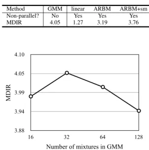
TABLE I: Average MDIR [dB] of each method Method GMM linear ARBM ARBM+sm Non-parallel? No Yes Yes Yes
MDIR 4.05 1.27 3.19 3.76 3.88 3.94 3.99 4.05 4.10 16 32 64 128 M D IR Number of mixtures in GMM
Fig. 5: Average MDIR of the conventional GMM-based VC with varying the number of mixtures.
MDIR is, the better the VC performance. For the evalua-tion, as Eq. (20) indicates, we needed to use parallel data
{x(t),y(t) }T
t=1 of the source and the target speakers that was
aligned using dynamic programming. But again, note that all the speech data used for the training was NOT parallel. The MDIR was calculated for each frame from the parallel data of the 10 sentences, and averaged.
B. Comparison methods
It is difficult to evaluate the proposed method because most of the existing VC approaches use parallel data in training and it is not fair to compare our method, which does not use parallel data, with those methods. Nevertheless, a linear-transform-based approach, which has not been proposed so far, presents an interesting comparison. This approach is simple; the vectoryˆ(t)is calculated as
ˆ y(t)
,AyA−x1(x
(t)
−bx) +by, (21) which was derived under the assumption thatx(t)=A
xv(t)+ bxandyˆ(t)=Ayv(t)+by, which means the acoustic features of each speaker are generated from the neutral acoustic fea-turesv(t)projected to the speaker using the adaptation matrix Ax orAy. The parametersAx,Ay,bx, andby are estimated using stochastic gradient decent just the same as our proposed method.
Just for a reference, we also compared our approach with a popular GMM-based VC method using parallel data of 40 sentences as a VC method based on parallel training (the VC type as in Fig. 1 (a)). We changed the number of mixtures M to 16, 32, 64, and 128. In our experiments, we found that M = 32performed best, as shown in Fig. 5.
Table I summarizes the VC experimental results, com-paring non-parallel-training-based VC methods (we refer to this as non-parallel VC), such as ‘linear’, ‘ARBM’ for our model without softmax constraints, and ‘ARBM+sm’ for our
1 2 3 4 5
Speaker identity Speech quality 2.68 3.58 3.61 1.55 2.65 3.95 MOS GMM linear ARBM
Fig. 6: Average MOS w.r.t. speaker specificity and speech quality for each method.
model with softmax constraints, and a supplementary parallel-training-based VC method (we refer to this as parallel VC), ‘GMM’. Each method was best-conditioned; choosing the number of hidden units H for our method will be discussed in the following section. For our method, we used the best-condition ofH = 8for the models with and without softmax constraints, which were trained using only the source and the target speakers’ speech unless otherwise noted. As shown in Table I, when we compare the results of non-parallel VC methods, we obtained a relatively low MDIR with the linear approach (‘linear’). However, the MDIR dramatically increased by almost two points when the existence of the latent phonological information was considered (‘ARBM’). The soft-max constraints further increased the MDIR (‘ARBM+sm’). This is because the ARBM with softmax constraints helped to represent the phonological information behind the speech data. Interestingly, the performance of our model was close to that of the parallel VC, which benefits from the parallel data, which is restricted to match the frames of the source and the target features. Our non-parallel approach produced results similar to that of the parallel approach without having such a benefit.
C. Subjective evaluation
We also conducted a subjective evaluation using mean opinion score (MOS) listening tests. Since we are interested in the spectral conversion, the converted speech of each method was generated from the obtained mel-cepstral features followed by conversion into signals with the original target’s F0 and aperiodic features. In this evaluation, eight participants listened to 10 sets of the original target speech (generated from analysis-by-synthesis) and the converted speech for each method (our method, the linear-based non-parallel approach, and the conventional GMM-based approach), and then selected how close the converted speech sounded to the original speech on a 5-point scale (5: excellent; 4: good; 3: fair; 2: poor; and 1: bad) with respect to speaker specificity and speech quality. The results are shown in Fig. 6. Compared with GMM, our method had slightly lower MOS w.r.t. speaker identity but almost the same MOS w.r.t. speech quality. In the linear
2.40 2.70 3.00 3.30 3.60 2 4 8 16 32 M D IR
Number of hidden units in ARBM
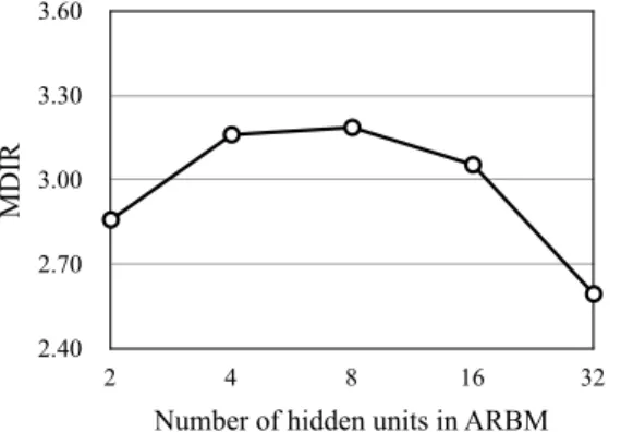
Fig. 7: Average MDIR of our method without softmax con-straints with varying the number of hidden units.
2.40 2.80 3.20 3.60 4.00 2 4 8 16 32 M D IR
Number of hidden units in ARBM+sm
Fig. 8: Average MDIR of our method with softmax constraints with varying the number of hidden units.
approach, the generated speech was very close to the original speech of the source speaker. That is why it produced a rather low MOS w.r.t. speaker identity, and high speech quality. In our approach, on the other hand, even though it does not use any parallel data in training, it produced similar MOS scores to the VC method, which uses parallel data in training. The speech data above will be available on our website4.
D. Number of hidden units
In this section, we see the effects of changing the number of hidden units in our model. Figs. 7 and 8 show the results with-out and with softmax constraints, respectively, when changing the number of hidden units as 2, 4, 8, 16, and 32. Through the experiments, we found that the results were rather varied even if the same number of hidden units were used; hence we took the best performance in several trials for each condition. The reasons will be discussed later. As shown in Figs. 7 and 8, the optimal numbers were around 8 in both cases, and the performance degraded as the number of hidden units increased. This is considered to be due to the fact that the model with more hidden units better represents the speech data; meanwhile it makes more spaces in hidden units to represent speaker-dependent information, and hence it cannot convert the voice
4http://www.sd.is.uec.ac.jp/nakashika
TABLE II: Average MDIR [dB] of our model w/o softmax in src-to-tar transformation (conversion) and tar-to-tar transfor-mation (reconstruction).
# of hidden units src-to-tar tar-to-tar
H= 8 3.35 4.98
H= 32 2.60 6.41
properly. To prove this, we reconstructed the target speech using our model; i.e., we input the acoustic features of the target speaker’s speech to the ARBM, calculated the hidden unit activations using the speaker-dependent parameters of the target speaker, and calculated the acoustic features from the hidden units using the target speaker’s parameters again. The results of the reconstruction are shown in the column of ‘tar-to-tar’ in Table II. As shown in Table II, when we gave more hidden units as H = 32, the MDIR of ‘tar-to-tar’ increased considerably (in other words, the reconstruction error decreased). Meanwhile in the conversion from the source to the target (‘src-to-tar’), the model with H = 32 had poor performance. Besides, the result in the case with H = 32 shows the interesting potential of our model. If we could obtain the true distribution of the phonological information (hidden units), the proposed method would produce a considerably high performance in VC.
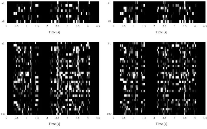
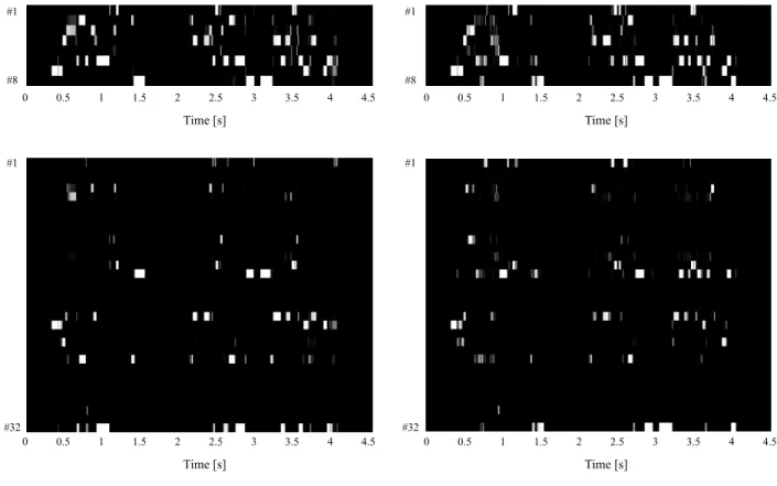
We further visually analyzed the effect of the number of hidden units. Fig. 9 shows examples of the distribution of the hidden units without softmax constraints, comparing the cases where H = 8 and H = 32 hidden units were used. The left and the right columns in Fig. 9 indicate the distribution calculated from the source speaker’s speech using the source speaker’s parameters, and from the target speaker’s speech using the target speaker’s parameters, respectively. In the case of H = 8, the two distributions are similar to each other, compared with the case of H = 32, where the two distributions are relatively different from each other. With softmax constraints, the two distributions are closer to each other as shown in Fig. 10 in both cases, which improved the average MDIR. Therefore, we can conclude that the following factors are important to improving the MDIR:
• high representation ability (with more hidden units) • closeness of the hidden unit distributions between the
source and the target speakers,
though there is a tradeoff between them, especially without softmax constraints.
E. Spectral analysis
Fig. 11 shows the comparison of the spectrograms of the converted speech using our method with softmax constraints (Fig. 11 (b)) and the target speech (Fig. 11 (c)) using a sentence selected from the evaluation sets. The converted spectrogram came from the source speaker’s spectrogram as shown in Fig. 11 (a). Note that the source and the target spectrograms in Fig. 11 were calculated from their mel-cepstral features for comparison. For clarity, Figs. 12 and 13 illustrate some examples of the spectra.
0 0.5 1 1.5 2 2.5 3 3.5 4 4.5 #1 #8 #1 #32 Time [s] #1 #8 #1 #32 0 0.5 1 1.5 2 2.5 3 3.5 4 4.5 Time [s] 0 0.5 1 1.5 2 2.5 3 3.5 4 4.5 Time [s] 0 0.5 1 1.5 2 2.5 3 3.5 4 4.5 Time [s]
(a) From the source speaker (b) From the target speaker
Fig. 9: The probability distribution of hidden units p(h|v,s) given the source speaker’s features (a) and the target speaker’s features (b) of the same sentence “Arayuru genjitsu o subete jibuN no ho: e nejimagetanoda” when H = 8 (upper row) and H = 32(lower row) hidden units without softmax constraints are used. The white and the black indicate the high and the low probability, respectively.
As shown in Figs. 11, 12 and 13, we can say that the converted spectrum more or less captures the characteristics of the target speaker’s spectrum. This is seen clearly in Figs. 12 and 13, where the frequencies of the spectral peaks (formant information) of the converted spectra are similar to those of the target speaker. Our proposed method has a great advantage in that even though we did not train a model of the direct conversion from the source to the target speakers and never used parallel data during the training, the source speech was converted into that of the target speaker.
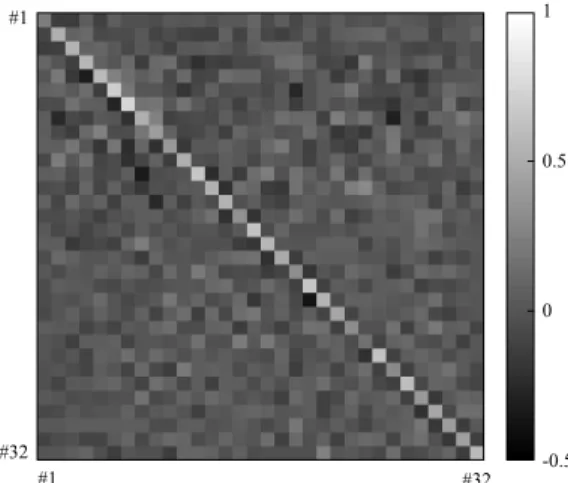
The actually estimated parameters Ax, Ay, and W¯ are shown in Figs. 14, 15, and 16, respectively. Interestingly, the tridiagonal elements loom over the matrices in Figs. 14 and 15. In some literature, such as [28], [29], [30], it is known that warping cepstral-based features between different speakers is achieved by linear transformation with an adaptation matrix, and tridiagonal elements of the adaptation matrix are sufficient for warping when mel-cepstral features are used. We obtained such characteristics in unsupervised learning.
F. Adding speech from more people
As noted before, the speaker-independent parameters in our model will be improved using speech data of more than the source and the target speakers. In this section, we report the results when the number of persons included in the training
speech data is changed without softmax constraints as shown in Fig. 17. We found that the MDIR improved as the number of persons increased up to 8, but did not improve so much beyond 8. This is considered to be due to the way of training, which is based on stochastic gradient decent. Assume that the numbers of training data for each person are all the same; i.e. the probability of the number of appearance of the speakerr in a minibatch is multinomial-distributed with the probability p(r) = 1
R inB =B0·Rtrials, whereR,B, andB0denote the numbers of persons, total batchsize, and batchsize per person, respectively. In this case, the expected value of the number of training data of the speaker r in the batch (we refer to this number as “the number of selection”) becomes B ·p(r) = B0, which means the number of selections does not change
as the number of persons increased. However, the variance of the number of selection is calculated as B·p(r)·(1− p(r)) =B0(1−R1). This indicates that the number of selection
gradually varies more as the number of persons increases. The stochastic gradient decent updates parameters just based on that batch; hence, the speaker-independent parameters become biased and are updated improperly as the number of persons increases, which leads to poor the MDIR.
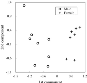
Fig. 18 shows the distribution of the learnt speaker-dependent parameters (A,B, andC) whenR= 16 persons’ speech was used that is projected into the two most principal
0 0.5 1 1.5 2 2.5 3 3.5 4 4.5 #1 #8 #1 #32 Time [s] #1 #8 #1 #32 0 0.5 1 1.5 2 2.5 3 3.5 4 4.5 Time [s] 0 0.5 1 1.5 2 2.5 3 3.5 4 4.5 Time [s] 0 0.5 1 1.5 2 2.5 3 3.5 4 4.5 Time [s]
(a) From the source speaker (b) From the target speaker
Fig. 10: The probability distribution of hidden unitsp(h|v,s)given the source speaker’s features (a) and the target speaker’s features (b) of the same sentence “Arayuru genjitsu o subete jibuN no ho: e nejimagetanoda” when H = 8 (upper row) and H = 32(lower row) hidden units with softmax constraints are used. The white and the black indicate the high and the low probability, respectively.
spaces using principal component analysis (PCA) with the notation of male or female for each. The most interesting point from Fig. 18 is that it can be easily devided into male and female groups in the first principal component even though they are trained in an unsupervised manner. This agrees with the intuition that when we try to recognize the identities of speakers, we feel the differences between the genders larger than the differences between individual persons. Another important point in Fig. 18 is that some individuals are categorized together, which implies that our model may be applicable to speaker clustering techniques, such as cluster adaptive training (CAT) [31].
V. CONCLUSION
In this paper, we presented a voice conversion (VC) method using a structured energy-based probabilistic model called an adaptive restricted Boltzmann machine (ARBM) aiming at non-parallel training, where no parallel data is required during the training. Compared with most existing VC approaches, which are based on parallel training, the non-parallel training is difficult and challenging because there are no restrictions on the frame-wise matching of the related acoustic features of the source and the target speakers under phonological supervision. Nevertheless, such non-parallel approaches have attractive advantages; theoretically, the texts of the speech data used
for the training do not have to be the same for both speakers, the trained parameters can be reused in the conversion of any other speaker pairs, and there is no need to make alignment that takes some efforts. Our experimental results showed that the proposed method produced results similar to that of the popular parallel-training approach, GMM, in regard to both objective and subjective criteria. Since the proposed model is designed for unsupervised separation of speaker-specific features and speaker-independent, phonological-related infor-mation from the observed acoustic features, it may be appli-cable to various other tasks, such as speaker identification, speech recognition, noise reduction, and controlling emotions in speech, which will be the focus of future work.
Contrary to our expectation, the large number of persons in training did not always help to estimate speaker-independent parameters and improve the performance. Many reasons could be considered; however, the learning method of stochastic gradient decent should be one of the reasons. We will consider using other learning techniques such as stochastic average gradient (SAG) [32] in the future.
REFERENCES
[1] A. Kain and M. W. Macon, “Spectral voice conversion for text-to-speech synthesis,” in Proc. IEEE Int. Conf. Acoust., Speech, Signal Process. (ICASSP), 1998, pp. 285–288.
8 0 4 6 2 1 3 5 7 0 0.5 1 1.5 2 2.5 3 3.5 4 4.5 8 0 4 6 2 1 3 5 7 0 0.5 1 1.5 2 2.5 3 3.5 4 4.5 8 0 4 6 2 1 3 5 7 0 0.5 1 1.5 2 2.5 3 3.5 4 4.5 Time [s] Time [s] Time [s]
F re que nc y [kH z]
(a) Source spectrogram (b) Converted spectrogram (c) Target spectrogram
Fig. 11: Spectrograms of the sentence “arayuru genjitsu o subete jibuN no ho: e nejimagetanoda” uttered by the souce speaker (a), converted from the source to the target speakers using our method (b), and utterd by the target speaker (c). The white and the black indicate the high and the low amplitude, respectively.
-20 -40 -60 -80 -100 0 1 2 3 4 5 6 7 8 Frequency [kHz] Target spectrum Converted spectrum Source spectrum A m pl it ude [dB] 0 -120
Fig. 12: The source, the converted, and the target spectra at the time 0.5 [s] from Fig. 11. The solid, the bold, and the dotted lines indicate the spectra of the target, the converted, and the source speech, respectively.
[2] C. Veaux and X. Robet, “Intonation conversion from neutral to expres-sive speech,” inProc. Interspeech, 2011, pp. 2765–2768.
[3] K. Nakamura, T. Toda, H. Saruwatari, and K. Shikano, “Speaking-aid systems using GMM-based voice conversion for electrolaryngeal speech,”Speech Communication, vol. 54, no. 1, pp. 134–146, 2012. [4] L. Deng, A. Acero, L. Jiang, J. Droppo, and X. Huang,
“High-performance robust speech recognition using stereo training data,” in
Proc. IEEE Int. Conf. Acoust., Speech, Signal Process. (ICASSP), 2001, pp. 301–304.
[5] A. Kunikoshi, Y. Qiao, N. Minematsu, and K. Hirose, “Speech genera-tion from hand gestures based on space mapping,” inProc. Interspeech, 2009, pp. 308–311.
[6] R. Gray, “Vector quantization,”IEEE ASSP Magazine, vol. 1, no. 2, pp. 4–29, 1984.
[7] H. Valbret, E. Moulines, and J.-P. Tubach, “Voice transformation using PSOLA technique,”Speech Communication, vol. 11, no. 2, pp. 175–187, 1992.
[8] Y. Stylianou, O. Capp´e, and E. Moulines, “Continuous probabilistic transform for voice conversion,”IEEE Trans. Speech and Audio Pro-cess., vol. 6, no. 2, pp. 131–142, 1998.
[9] T. Toda, A. W. Black, and K. Tokuda, “Voice conversion based on maximum-likelihood estimation of spectral parameter trajectory,”IEEE
-20 -40 -60 -80 -100 0 1 2 3 4 5 6 7 8 Frequency [kHz] Target spectrum Converted spectrum Source spectrum A m pl it ude [dB] 0 -120
Fig. 13: The source, the converted, and the target spectra at the time 1.5 [s] from Fig. 11. The solid, the bold, and the dotted lines indicate the spectra of the target, the converted, and the source speech, respectively.
Trans. Audio, Speech, and Lang. Process., vol. 15, no. 8, pp. 2222–2235, 2007.
[10] E. Helander, T. Virtanen, J. Nurminen, and M. Gabbouj, “Voice conver-sion using partial least squares regresconver-sion,”IEEE Trans. Audio, Speech, and Lang. Process., vol. 18, no. 5, pp. 912–921, 2010.
[11] N. M. Daisuke Saito, Hidenobu Doi and K. Hirose, “Application of matrix variate Gaussian mixture model to statistical voice conversion,” inProc. Interspeech, 2014, pp. 2504–2508.
[12] R. Takashima, T. Takiguchi, and Y. Ariki, “Exemplar-based voice conversion in noisy environment,” in Proc. IEEE Spoken Language Technology Workshop (SLT), 2012, pp. 313–317.
[13] R. Takashima, R. Aihara, T. Takiguchi, and Y. Ariki, “Noise-robust voice conversion based on spectral mapping on sparse space,” inSSW8, 2013, pp. 71–75.
[14] S. Desai, E. V. Raghavendra, B. Yegnanarayana, A. W. Black, and K. Prahallad, “Voice conversion using artificial neural networks,” in
Proc. IEEE Int. Conf. Acoust., Speech, Signal Process. (ICASSP), 2009, pp. 3893–3896.
[15] L. H. Chen, Z. H. Ling, Y. Song, and L. R. Dai, “Joint spectral distribution modeling using restricted Boltzmann machines for voice conversion,” inProc. Interspeech, 2013, pp. 3052–3056.
1 0.5 0 -0.5 #1 #32 #1 #32
Fig. 14: Estimated adaptation matrix for the source speaker
Ax. 1 0.5 0 -0.5 #1 #32 #1 #32
Fig. 15: Estimated adaptation matrix for the target speakerAy.
machine for voice conversion,” inProc. ChinaSIP, 2013.
[17] T. Nakashika, R. Takashima, T. Takiguchi, and Y. Ariki, “Voice con-version in high-order eigen space using deep belief nets,” in Proc. Interspeech, 2013, pp. 369–372.
[18] T. Nakashika, T. Takiguchi, and Y. Ariki, “Voice conversion using RNN pre-trained by recurrent temporal restricted Boltzmann machines,”
IEEE/ACM Trans. Audio, Speech, and Lang. Process., vol. 23, no. 3, pp. 580–587, 2015.
[19] A. Mouchtaris, J. Van der Spiegel, and P. Mueller, “Nonparallel training for voice conversion based on a parameter adaptation approach,”IEEE Trans. Audio, Speech, and Lang. Processs, vol. 14, no. 3, pp. 952–963, 2006.
[20] C.-H. Lee and C.-H. Wu, “Map-based adaptation for speech conversion using adaptation data selection and non-parallel training,” in Proc. Interspeech, 2006, pp. 2254–2257.
[21] T. Toda, Y. Ohtani, and K. Shikano, “Eigenvoice conversion based on Gaussian mixture model,” inProc. Interspeech, 2006, pp. 2446–2449. [22] D. Saito, K. Yamamoto, N. Minematsu, and K. Hirose, “One-to-many
voice conversion based on tensor representation of speaker space,” in
Proc. Interspeech, 2011, pp. 653–656.
[23] G. E. Hinton, S. Osindero, and Y. W. Teh, “A fast learning algorithm for deep belief nets,”Neural computation, vol. 18, no. 7, pp. 1527–1554, 2006.
[24] K. Cho, A. Ilin, and T. Raiko, “Improved learning of Gaussian-Bernoulli restricted Boltzmann machines,” inProc. ICANN. Springer, 2011, pp. 10–17.
[25] R. Salakhutdinov, A. Mnih, and G. Hinton, “Restricted Boltzmann machines for collaborative filtering,” inProceedings of the 24th inter-national conference on Machine learning. ACM, 2007, pp. 791–798.
1 0.5 0 -0.5 1.5 -1 -1.5 #1 #8 #1 #32
Fig. 16: Estimated speaker-independent matrixW¯ .
2.90 3.08 3.25 3.43 3.60 2 4 8 16 M D IR Number of persons
Fig. 17: Average MDIR of our method with changing the number of persons used in the training.
[26] K. Sohn, D. Y. Jung, H. Lee, and A. O. H. III, “Efficient learning of sparse, distributed, convolutional feature representations for object recognition,” in Proc. IEEE International Conference on Computer Vision (ICCV). IEEE, 2011, pp. 2643–2650.
[27] M. Morise, “An attempt to develop a singing synthesizer by collaborative creation,” inProc. the Stockholm Music Acoustics Conference (SMAC), 2013, pp. 287–292.
[28] M. Pitz and H. Ney, “Vocal tract normalization equals linear trans-formation in cepstral space,”IEEE Transactions on Speech and Audio Processing, vol. 13, no. 5, pp. 930–944, 2005.
[29] E. Variani and T. Schaaf, “VTLN in the MFCC domain: Band-limited versus local interpolation,” inProc. Interspeech, 2011, pp. 1273–1276. [30] T. Emori and K. Shinoda, “Vocal tract length normalization using rapid maximum-likelihood estimation for speech recognition,” Systems and Computers in Japan, vol. 33, no. 5, pp. 30–40, 2002.
[31] M. J. Gales, “Multiple-cluster adaptive training schemes,” inProc. IEEE Int. Conf. Acoust., Speech, Signal Process. (ICASSP), vol. 1. IEEE, 2001, pp. 361–364.
[32] M. Schmidt, N. L. Roux, and F. Bach, “Minimizing finite sums with the stochastic average gradient,”arXiv, 2013.
-1.1 -0.6 -0.1 0.4 0.9 1.4 -1.8 -1.2 -0.6 0 0.6 1.2 2nd c om pone nt 1st component Male Female
Fig. 18: A scatter of speaker-dependent parameters of 16 persons in two dimensional principals.
PLACE PHOTO HERE
Toru Nakashikareceived his B.E. and M.E. degrees in computer science from Kobe University in 2009 and 2011, respectively. On the summer in 2010, he was a student researcher at IBM Research, Tokyo Research Laboratory. From September 2011 to Au-gust 2012, he was a visiting researcher in the image group at INSA de Lyon in France. In the same year, he continued his research as a doctoral student at Kobe University, and received his Dr.Eng. degree in computer science in 2014. To April 2015, he was an Assistant Professor at Kobe University. He is currently an Assistant Professor at the University of Electro-Communications. He recieved the IEICE ISS Young Researcher’s Award in Speech Field in 2013. He is a member of IEEE, IEICE and ASJ.
PLACE PHOTO HERE
Tetsuya Takiguchi received the B.S. degree in applied mathematics from Okayama University of Science, Okayama, Japan, in 1994, and the M.E. and Dr. Eng. degrees in information science from Nara Institute of Science and Technology, Nara, Japan, in 1996 and 1999, respectively. From 1999 to 2004, he was a researcher at IBM Research, Tokyo Research Laboratory, Kanagawa, Japan. He is currently an associate professor at Kobe University. His research interests include statistic signal processing and pat-tern recognition. He received the Awaya Award from the Acoustical Society of Japan in 2002. He is a member of the IEEE, the IPSJ, and the ASJ.
PLACE PHOTO HERE