Economics Working Paper Series
2020/007
exuber: Recursive Right-Tailed Unit Root Testing
with R
Kostas Vasilopoulos, Efthymios Pavlidis
and Enrique Martínez-García
The Department of Economics
Lancaster University Management School
Lancaster LA1 4YX
UK
© Authors
All rights reserved. Short sections of text, not to exceed two paragraphs, may be quoted without explicit permission,
provided that full acknowledgement is given. LUMS home page: http://www.lancaster.ac.uk/lums/
exuber
: Recursive Right-Tailed Unit Root Testing
with R
Kostas Vasilopoulos Lancaster University Efthymios Pavlidis Lancaster University Enrique Mart´ınez-Garc´ıaFederal Reserve Bank of Dallas
Abstract
This paper introduces the R packageexuberfor testing and date-stamping periods of mildly explosive dynamics (exuberance) in time series. The package computes test statis-tics for the supremum ADF test (SADF) of Phillips, Wu, and Yu(2011), the generalized SADF (GSADF) of Phillips, Shi, and Yu (2015a,b), and the panel GSADF proposed by Pavlidis, Yusupova, Paya, Peel, Mart´ınez-Garc´ıa, Mack, and Grossman (2016); gen-erates finite-sample critical values based on Monte Carlo and bootstrap methods; and implements the corresponding date-stamping procedures. The recursive least-squares al-gorithm that we introduce in our implementation of these techniques utilizes the matrix inversion lemma and in that way achieves significant speed improvements. We illustrate the speed gains in a simulation experiment, and provide illustrations of the package using artificial series and a panel on international house prices.
Keywords: Mildly explosive time series, Right-tailed unit root tests, R.
1. Introduction
Over the last decades, and especially after the financial crisis of 2007-08, a large interest has developed in econometric tests of exuberance in asset markets. The objective of these tests is to detect periods in which the data generating process of a macroeconomic or a financial variable is characterized by (mildly) explosive dynamics. Because such periods are typically followed by large market corrections which can trigger economic recessions, exuberance tests are of prime importance for academics, who want to shed light on the functioning of asset markets, but also for policymakers for monitoring purposes. Applications of exuberance tests include, among others, stock prices, real estate valuations, precious metals, foreign exchange rates, crypto-currencies, public debt, and bond yield spreads.
Early empirical studies on exuberance adopted linear, time-invariant model specifications. The majority of these studies tested for explosive behaviour by applying standard right-tailed unit root tests, such as the Augmented Dickey Fuller (ADF), to the entire sample of available data. Although widely employed, standard unit root tests have extremely low power in detecting episodes of explosive dynamics when these are interrupted by market crashes (Evans 1991).
In recent years, several new econometric methodologies have been proposed to deal with this shortcoming. Two methodologies that have gained increasing popularity are the SADF of
Phillipset al. (2011) and the GSADF proposed by Phillipset al. (2015a,b). In order to deal with the effect of a collapse in a time series on the test’s performance, the SADF and GSADF
methodologies involve a recursively evolving algorithm that estimates ADF regressions on subsamples of data. The SADF procedure sequentially tests for explosive behaviour by using a forward expanding window, while its extension, the GSADF, tests for exuberance using all possible subsamples of a time series given a user-specified minimum window size.
The GSADF procedure is particularly attractive because it minimizes the impact of previ-ous boom-bust episodes on the current identification and thereby is consistent with multiple changes in regime. Simulation evidence inHomm and Breitung(2012),Phillipset al.(2015a) andPavlidis, Paya, and Peel(2017) suggests that the test has accurate size and higher power compared to alternative tests for changes in persistence.1 Another attractive feature of the GSADF methodology is that, due to its recursive nature, it allows date-stamping of the ex-act periods, if any, during which the series under examination displays explosive dynamics. Therefore, it can be used to shed light on past episodes of exuberance but also for real time market surveillance.
Both the SADF and GSADF are univariate testing procedures and, thus, only allow drawing conclusions at the unit level. In several occasions, exuberance is almost coincident across a group of assets. Prime examples include regional and international house prices in the 2000s (see Pavlidis et al. 2016; Greenaway-McGrevy, Grimes, and Holmes 2019) and stock prices (Narayan, Mishra, Sharma, and Liu 2013). To accommodate concurrent episodes of exuberance, Pavlidis et al.(2016) propose an extension of the GSADF procedure to a panel setting. The panel GSADF draws inference on the presence of overall exuberance by exploiting the cross-sectional dimension of a dataset through a sieve bootstrap procedure. This extension can perform substantially better than univariate tests applied to aggregated series in the presence of synchronized episodes of exuberance, and like univariate tests, provides a date-stamping strategy (Pavlidis, Mart´ınez-Garc´ıa, and Grossman 2019).
In this paper, we introduce the R package exuber that deals with the detection of periods of mildly explosive dynamics (exuberance) in time series processes using the SADF, GSADF and panel GSADF methodologies. Two distinctive features of exuber are its computational speed and its ease of use. With regard to the first feature, the core function of the package recursively estimates ADF regressions by utilizing the Sherman–Morrison–Woodbury formula to efficiently update least-squares estimates as the sub-sample size changes. To improve further computational efficiency, this function is written in C++ using the Rcpp extension package and employsRcppArmadillo for high-performance linear algebra (Eddelbuettel and Fran¸cois 2011;Eddelbuettel 2013;Eddelbuettel and Sanderson 2014). As we show in Section
4, this implementation leads to computational speed gains of one or more orders of magnitude compared to other R packages dealing with exuberance. Computational speed is especially important for statistical inference. This is so because the distributions of the various test statistics of exuberance are non-standard and thus their estimation requires the use of Monte Carlo simulation or bootstrap methods. In addition to the recursive least squares algorithm, exuber exploits the facilities of R for parallel computing, via the packagesparallelandforeach, to compute critical values in a timely manner, even when the dimension of the dataset under examination is large. With respect to its functionality,exuberhas a simple and intuitive API, it can handle different data objects whose structure is wide, it allows for single index parsing, it enables easy manipulation of the estimated objects and, finally, it produces publication-ready graphs. The exuber package is currently employed by the Federal Reserve Bank of
1
These include the modified tests of Bhargava (1986), Busetti and Taylor (2004), Kim (2000), and the Chow-type unit root test examined byHomm and Breitung(2012)
Dallas and by the UK Housing Observatory for the production of exuberance indicators for UK regional and international housing markets.2 To demonstrate the functionality of the package and its ease of use, we provide two examples: one with artificial time series data and another with a panel of international house prices provided by the Federal Reserve Bank of Dallas (Mack, Mart´ınez-Garc´ıaet al.2011).
The rest of the paper is organized as follows. Section2gives an outline of the SADF, GSADF, and panel GSADF econometric methodologies. Section 3 provides an overview of the main functions and methods of the package, and Section4deals with the computational approach to estimation, software implementation, and performance. Section5 presents the two hands-on examples. Finally, the last section discusses future extensions of the package.
2. Econometric Methodologies
In this section, we provide a brief description of the SADF, GSADF and panel GSADF econo-metric methodologies, outline the associated date-stamping strategies, and discuss technical details about their implementation.
2.1. Univariate Right-Tailed Tests
At the heart of all the methodologies considered lies the following ADF regression equation, ∆yt=ar1,r2+γr1,r2yt−1+
Xk
j=1ψ j
r1,r2∆yt−j +t, (1)
where yt denotes a generic time series, ∆yt−j withj = 1, . . . , k are lagged first differences of
the series, included to accommodate serial correlation,t∼ N(0, σr21,r2), and ar1,r2,γr1,r2 and
ψrj1,r2 withj = 1, . . . , k are regression coefficients. The subscriptsr1 and r2 denote fractions
of the total sample size (ofT observations) that specify the starting and ending points of a subsample period.
We are interested in testing the null hypothesis of a unit root, H0 : γr1,r2 = 0, against the
alternative of explosive behavior inyt,H1 :γr1,r2 >0. The ADF test statistic corresponding
to this null hypothesis is given by ADFr2
r1 =γbr1,r2/s.e.(γbr1,r2). (2)
The Standard ADF Test
For the ADF test, the statistic in equation (2) is obtained by estimating regression (1) on the full sample of observations, i.e., by settingr1 = 0 andr2 = 1. Under the null of a unit root,
the limit distribution of ADF10 is given by,
R1 0 W dW R1 0 W2 1/2,
2Federal Reserve Bank of Dallas’ International House Price Database (
https://www.dallasfed.org/ institute/houseprice#tab2), International Housing Observatory (https://int.housing-observatory.com) and UK Housing Observatory (https://uk.housing-observatory.com).
whereW is a Wiener process. Testing for exuberance entails comparing the ADF10 statistic with the right-tailed critical value from its limit distribution. In this setting with r1 and r2
fixed at 0 and 1, respectively, the alternative hypothesis is that of exuberance over the entire sample. Because the standard ADF test is not consistent with changes in regime, it exhibits extremely low power in the presence of boom-bust episodes. In fact, nonlinear dynamics, such as those displayed by periodically-collapsing speculative bubbles, frequently lead to finding spurious stationarity even when the process under examination is inherently explosive (see
Evans 1991).
The SADF Test
Phillipset al.(2011) propose a methodology that is consistent with a single boom-bust episode. Their methodology involves estimating (1) using a forward expanding sample. In this setting, the beginning of the subsample is held constant atr1 = 0, while the end of the subsample,r2,
increases from r0 (the minimum window size) to one (the entire sample period). Recursive
estimation of (1) yields a sequence of ADFr2
0 statistics. The supremum of this sequence,
called the SADF statistic, is defined by,
SADF(r0) = sup r2∈[r0,1]
ADFr2 0 ,
and has a limit distribution given by, sup r2∈[r0,1] Rr2 0 W dW (Rr2 0 W2)1/2 .
Similarly to the standard ADF test, rejection of the null of a unit root requires that the SADF statistic exceeds the right-tailed critical value from its limit distribution. However, contrary to the standard ADF test which examines the presence of explosive dynamics during the entire period, the alternative hypothesis of the SADF test is that of explosive dynamics in some part(s) of the sample.
The Generalized SADF (GSADF) Test
More recently, Phillipset al. (2015a,b) proposed an extension of the SADF, the generalized SADF (GSADF), which has the same alternative hypothesis as the SADF but which covers a larger number of subsamples. Specifically, given a minimum window sizer0, the methodology
involves estimating regression (1) for all possible subsamples by allowing both the ending point, r2, and the starting point, r1, to change. This extra flexibility on the estimation
window results in substantial power gains and makes the GSADF test better suited to detect the presence of multiple changes in regime.
Formally, the GSADF statistic is defined as,
GSADF(r0) = sup
r2∈[r0,1],r1∈[0,r2−r0]
ADFr2
r1. (3)
and its limit distribution under the null is,
sup r2∈[r0,1],r1∈[0,r2−r0] 1 2rw[W(r2) 2−W(r 1)2−rw]− Rr2 r1 W(r)dr[W(r2)−W(r1)] r1/2w rw Rr2 r1 W(r) 2dr−hRr2 r1 W(r)dr i21/2 , (4)
where rw = r2−r1 is the size of the expanding window. Again, rejection of the unit root
hypothesis in favor of explosive behavior requires that the test statistic exceeds the right-tail critical value from its limit distribution.
Date-Stamping Strategies
If the null of a unit root in yt is rejected, then the SADF and GSADF methodologies can
provide a chronology of episodes of exuberance. For the SADF methodology, estimates of the origin and conclusion of exuberance can be obtained by comparing the time series of the recursive, backward ADF (BADF) test statistics against the right-tailed critical value of the distribution of the standard Dickey-Fuller statistic. Lettingre and rf correspond to the
origination and termination dates, respectively, these estimates can be constructed from,
b
re= inf r2∈[r0,1]
r2: ADFr02 > cuαr2 and brf = inf
r2∈[rbe,1]
r2 : ADFr02 < cuαr2 ,
wherecuαr2 is the 100(1−α)% critical value of the ADF statistic andαis the chosen significance level. A similar strategy is proposed by Phillips et al. (2015a,b) as part of the GSADF methodology. The strategy in this case is based on the sequence of backward SADF statistics,
BSADFr2(r0) = sup r1∈[0,r2−r0]
SADFr2
r1, (5)
and estimates the origination and termination dates according to,
b re= inf r2∈[r0,1] r2 : BSADFr2(r0)> scu α r2 and brf = inf r2∈[bre,1] r2 : BSADFr2(r0)< cu α r2 , where scuαbr
2Tc is the 100 (1−α) % critical value of the SADF for br2Tc observations. The
consistency of the SADF dating strategy in the presence of a single period of explosive dynam-ics in yt is established in Phillips et al. (2011), and the consistency of the GSADF strategy
with one or two explosive periods is established inPhillipset al. (2015a,b).
Technical Details
The computation of the recursive unit root test statistics necessitates the selection of the minimum window size, r0, and the autoregressive lag length, k. Regarding the minimum
window size, this has to be large enough to allow initial estimation, but it should not be too large to avoid missing short episodes of exuberance. Phillipset al. (2015a,b) recommend setting the minimum window size according to the rule of thumb: r0 = 0.01 + 1.8/
√
T. With respect to the selection of k, simulation evidence indicates the proposed right-tailed unit root methodologies work well when the number of lags is fixed at a small value, i.e., 0 or 1. On the contrary, lag selection based on information criteria can result in severe size distortions. The implementation of these right-tailed unit root tests also requires the limit distributions of the SADF, GSADF and BSADF test statistics. These distributions are non-standard and depend on the minimum window size. Consequently, critical values have to be obtained through either Monte Carlo simulations or bootstrapping.
2.2. The Panel GSADF Procedure
The SADF and GSADF tests can only be applied to individual time series and, hence, do not exploit the panel nature of many macroeconomic and financial datasets. Based on the work
of Im, Pesaran, and Shin (2003), Pavlidis et al. (2016) propose an extension of the GSADF procedure to heterogeneous panels.
Consider the panel version of regression equation (1), ∆yi,t =ai,r1,r2 +γi,r1,r2yi,t−1+
Xk
j=1ψ j
i,r1,r2∆yi,t−j+i,t, (6)
where i = 1, . . . , N denotes the panel index, and the remaining variables are defined as in the previous sub-section. The panel GSADF test examines the null hypothesis of a unit root, H0 : γi,r1,r2 = 0, in all N series against the alternative of explosive behavior in a subset of
series, H1 : γi,r1,r2 > 0 for some i. This alternative allows for γi,r1,r2 to differ across panels
and, in that sense, is more general than approaches that impose a homogeneous alternative hypothesis. The testing procedure involves constructing a measure of overall exuberance by averaging the individual BSADF statistics at each time period,
panel BSADFr2(r0) =
1 N
XN
i=1BSADFi,r2(r0). (7)
Given (7), the definition of the panel GSADF statistic follows naturally. It is simply the supremum of the panel BSADF,
panel GSADF (r0) = sup r2∈[r0,1]
panel BSADFr2(r0). (8)
Like for the univariate methods, testing for and dating episodes of overall exuberance involves comparing the panel GSADF and panel BSADF statistics with the right-tailed critical values from the corresponding limit distributions. However, as shown by Maddala and Wu (1999) and Chang (2004), the limit distribution of panel unit root tests based on mean unit root statistics is not invariant to cross-sectional dependence of the error terms, i. To this end,
the authors adopt a sieve bootstrap that is designed specifically to allow for cross-sectional error dependence. Details of the sieve bootstrap algorithm can be found in the Appendix of
Pavlidiset al. (2016).
3. Installation and Package Overview
The package exuber is available on the Comprehensive R Archive Network (CRAN) at
https://CRAN.R-project.org/package=exuber, and can be installed and accessed from the R console. The package has a number of dependencies on other R packages, which are automatically loaded withexuber. The main dependencies include Rcpp (Eddelbuettel 2013), parallel(R Core Team 2020),foreach(Microsoft and Weston 2020), dplyr(Wickham, Fran¸cois, Henry, and M¨uller 2020) and purrr(Henry and Wickham 2020).
R> install.package("exuber") R> library(exuber)
exuber centers around the function radf(). This function takes as input three arguments
(data, minw, lag) and returns a list containing ADF, SADF, GSADF, BADF, BSADF, panel GSADF and panel BSADF test statistics. With regard to the first argument,exuberis capable of working with regulardata.frame,ts, numeric vector ormatrix classes without
the need for any further transformation. Estimation always includes a time dimension, and in the case of multiple time series a cross-sectional dimension. In line with the convention in time-series econometrics, the required format is wide, where each row corresponds to a unique time period and each column represents a time series. Theradf()function is vectorized, i.e., it can handle multiple series at once, to improve efficiency. This property also enables the computation of panel statistics internally as a by-product of the univariate estimations with minimal additional cost incurred. When the data input is a data.frame with an explicit
class-Datecolumn, exuber uses a similar principle as tsibble(Wang, Cook, and Hyndman 2020) for index-search and parsing. In all other cases, anintegerindex is automatically cre-ated. The index is used byexuber’s methods for date-stamping and plotting. The arguments
minw and lagspecify the minimum window size and the lag length used in estimation. The default values for these arguments are set equal to the value suggested by the rule ofPhillips
et al.(2015a),bT(0.01 + 1.8/p(T)c, and zero, respectively. The functionradf() returns an object of classradf_obj.
The functions radf_mc_cv(), radf_wb_cv(), and radf_sb_cv() generate 90%, 95%, and 99% critical values for different sample and minimum window sizes. The three functions for generating critical values return an object of class radf_cv. The function radf_mc_cv()
generates finite-sample critical values for univariate unit root tests approximating the Brow-nian motion processes in the limiting functionals specified in Section2by using independent N(0,1) random variates. While, functionsradf_wb_cv() and radf_sb_cv() implement the univariate wild bootstrap and the panel sieve bootstrap methodologies outlined in Harvey, Leybourne, Sollis, and Taylor (2016) and Pavlidis et al. (2016). The default values for the number of Monte Carlo and bootstrap repetitions inexuber is set to 500. Users can also ob-tain the entire distribution of the various test statistics by using the corresponding functions
radf_mc_distr(),radf_wb_distr()andradf_sb_distr(), which return an object of class
radf_distr.
Because the majority of users employ Monte Carlo critical values and adopt the default minimum window size,exubercomes with a stored dataset of critical values for sample sizes of up to 600 observations. These critical values can be replicated with theradf_mc_cv()function by setting the number of repetitionsnrepto 2000 and theseedto 123. For applications which involve series of length between 600 and 2000 observations, critical values can be obtained from the exuberdata package. Due to CRAN restrictions on package size, exuberdata is instead distributed through the ‘Drat’ R Archive Template (Eddelbuettel 2019), that works seamlessly withexuber, does not depend onRtools, and makes it easy for package installation and upgrades.3
Several methods are used to process the output ofradf(), together with the output of one of the functions for generating critical values. The use of S3 methods reflects our preference for software scalability, as we intend to include new econometric methodologies in future versions of the package. The methodsummary()returns a table of the estimated ADF, SADF, GSADF test statistics together with the corresponding critical values for each individual series indata. When the cross-sectional dimension of the dataset is large, the output of summary() can become lengthy and its interpretation tedious. In such cases, the user can work directly with objectsradf_objand radf_cv(as we will demonstrate in Section5) or alternatively use the methoddiagnostics(). For each series in a panel,diagnostics() compares the estimated
3
Theexuberdatapackage is hosted athttps://github.com/kvasilopoulos/exuberdataand can be easily installed using the wrapper function in exuber,install_exuberdata().
SADF or GSADF test statistic to the corresponding set of critical values and reports whether the null of a unit root is rejected and, if so, at which level of significance.
Date-stamping is implemented via the methoddatestamp(). This method produces an object of classds_radfwhich contains the estimates of the origination, termination and duration of episodes of exuberance. To prevent wrong application of the testing procedure, datestamp()
only reports results for series for which the first-stage test statistic is significant and when all series are non-explosive prints a message to notify the user. In some applications, researchers may want to exclude very short episodes of exuberance by setting a minimum duration period. The package exuber does not set a minimum duration for periods of exuberance by default. However, minimum duration requirements can be introduced as a refinement at the discretion of the user by altering the value of the argument min_duration. Phillips et al. (2015a,b) recommend two rules for setting the minimum duration, which can be computed using the helper functionpsy_ds().
To produce publication-ready graphs,exuber uses theggplot2::autoplot generic for plot-ting objects of classesradf_obj,ds_radf, andradf_distr. An attractive feature of this im-plementation is that it allows users to exploit the common features from theggplot2package to manipulate plots. augmentandaugment_joinmethods are also provided that manipulate the data into a convenient format for custom plotting. For class radf_objobjects, autoplot()
produces a faceted plot displaying BSADF statistics together with the corresponding sequence of critical values. For classds_radf objects, autoplot() uses geom_segment() to produce a ‘chronology’ plot which displays a set of segmented horizontal lines, with each line rep-resenting the identified periods of exuberance for an individual series. If the data input in
radf()includes aDateindex then this is automatically passed toautoplot.radf_obj()and
autoplot.ds_radf()and used in the creation of x-axes.
Finally, exuber provides functions for simulating data from popular bubble data generating processes. These include the periodically-collapsing bubble processes ofBlanchard(1979) and
Evans(1991), and the one- and two-bubble processes proposed byPhillipset al. (2015a).
4. Computational Approach to Estimation and Performance
The implementation of the right-tailed unit root testing procedures outlined in Section 2
requires the application of iterative routines which repeatedly fit ADF regression equation (1) on subsamples of data by solving a sequence of otherwise standard least-squares problems. By replacing the sample fractionsr1 and r2 with their discrete time analogues, t1 and t2, the
ADF regression equation can be rewritten in matrix form as,
Yt1:t2 =Xt1:t2βt1:t2+Et1:t2, (9) where Yt1:t2 = ∆yt1 ∆yt1+1 .. . ∆yt2 , Xt1:t2 = xt1 xt1+1 .. . xt2 = 1 yt1−1 ∆yt1−1 · · · ∆yt1−k 1 yt1 ∆yt1 · · · ∆yt1−k+1 .. . ... ... · · · ... 1 yt2−1 ∆yt2−1 · · · ∆yt2−k ,
Et1:t2 = t1 t1+1 .. . t2 , andβt1:t2 = αt1:t2 γt1:t2 ψt11:t2 .. . ψtk1:t2 .
For a given subsample,t1:t2, the solution to the least squares problem,
argmin βt1:t2 ||Yt1:t2−Xt1:t2βt1:t2|| 2, (10) is given by, βt1:t2 = (X 0 t1:t2Xt1:t2) −1X0 t1:t2Yt1:t2. (11)
The main computational cost in estimating (11) and the coefficient standard errors, arises from the computation and inversion of the square matrixDt1:t2 = (X
0
t1:t2Xt1:t2). Because the
construction of Dt1:t2 takes O(nv
2) (wherev =k+ 2 is the number of regression parameters
and n=t2−t1+ 1 is the subsample size) and the inversion ofDt1:t2 typically requiresO(v 3),
the overall algorithmic complexity per iteration isO(v3+nv2). This cost may be acceptable in settings where the number of series and iterations is relatively small, but it makes the application of recursive unit root tests to long financial series and large panels cumbersome, and it becomes prohibitive for extensive power and size simulation experiments. To get a sense of the magnitude of this problem, consider a single series of T = 1000 observations and a minimum window size given by the rule of thumb in Section 2, i.e., m = 74. In this setting, the estimation of the SADF and GSADF tests requires T −m+ 1 = 935 and (T −m+ 1)(T −m+ 2)/2 = 437580 recursions, respectively, and the generation of critical values involves the computation of matrixDt1:t2 and its inverse hundreds of millions or billions
of times, depending on the number of Monte Carlo or bootstrap repetitions.
To reduce algorithmic complexity, the workhorse function of exuber employs a recursive-least squares method which incrementally updates Dt1:t2 from its previous value. Following
the standard notation in the statistics literature, letGt1:t2 =D
−1
t1:t2 denote the gain matrix.
Using the matrix inversion lemma, the gain matrix can be recursively computed from its previous value according to,
Gt1:t2 =Gt1:t2−1−(1 +xt2Gt1:t2−1x 0 t2) −1(G t1:t2−1x 0 t2)(xt2Gt1:t2−1), (12)
and the coefficient vector can be incrementally updated by, βt1:t2 =βt1:t2−1−Gt1:t2x
0
t2(xt2βt1:t2−1−∆yt2). (13)
The attractiveness of the above algorithm lies in the fact that it reduces the complexity of the problem from O(v3 +nv2) to O(v2), which only increases linearly with the number of recursions.
Software Implementation. For interpreted languages such as R, iterative function calls typically come with a heavy computational overhead due to high-level language properties like dynamic typing, bounds checking, and garbage collection (see, e.g.,Sridharan and Patel 2014). To avoid substantial speed penalties and obtain high-level computational efficiency, radf()
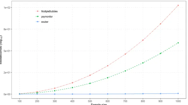
Figure 1: Package performance comparison.
is written in C++ using theRcpp extension package in conjunction withRcppArmadillofor high-performance linear algebra. As we show next, this implementation leads to substantial gains in computational efficiency.
Figure1displays the run-time performance ofexuberfor samples of sizeT ={100, . . . ,1000}, lag length k = 1, and a minimum window size of 30 observations. It also shows the per-formance of the two other R packages, psymonitor (Caspi, Phillips, and Shi 2018) and
MultipleBubbles4(Lacerda, Phillips, and Shi 2018), that provide right-tailed recursive unit root tests. Unlike exuber, these packages do not exploit the recursive nature of the problem at hand but instead use a batch least squares algorithm. Median times were generated on an Intel (R) Core(TM) i7-8700 CPU @3.20GHz with 64.0 GB RAM using 100 simulations, and collected using the microbenchmark package (Mersmann 2019). As is evident from the figure,exuber performs remarkably well both in absolute and relative terms, with the differ-ence in computation time across packages becoming particularly apparent as the sample size increases. For a sample size of 1000 observations, the computation time for exuber is 0.78 seconds, while for psymonitor and MultipleBubles it is 59.2 seconds (76 times slower) and 102.4 seconds (132 times slower), respectively.
The computational speed on the one hand and the recursive nature of our estimation algo-rithm on the other render parallel estimation for a single series nontrivial and unnecessary. Parallel computing is particularly beneficial, however, for statistical inference. exuber uses the package parallel and the looping construct offoreach to acquire the non-standard
finite-4The function
gsadf_sadf of MultipleBubbles does not allow for a user-specified minimum window size.
To provide meaningful comparisons across packages, in our simulation experiments we have used a slightly modified version of the function. The modification does not affect run-time performance.
sample distributions of the various test statistics via Monte Carlo or bootstrap simulations.
5. Examples with Artificial and Real Data
To demonstrate the functionality of the package, in this section we provide two applications. The first application involves an artificial series, while the second explores the presence of explosive dynamics in a panel of international house price data.
5.1. Simulated Bubble Series
For our first application, we simulate data from the one-bubble data generating process of
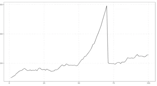
Phillipset al.(2015a) using the function psy1_sim(). This data generating process switches from a martingale to mildly explosive and then collapses back to a martingale at predetermined sample points. We consider a series of 100 observations, and set the start and end dates of the bubble period at observations 50 and 70. The time evolution of the series can be visualized in Figure2.
R> sim <- sim_psy1(120, te = 50, tf = 70, seed = 145) R> autoplot(sim)
Figure 2: Simulation of a single-bubble process.
To illustrate the ease of use ofexuberby non-expert users, we adopt the default values in the estimation of the unit root test statistics.
R> radf_sim <- radf(sim)
This produces an object of classradf_objthat contains the entire set of test statistics for the univariate testing procedures (i.e., the ADF, SADF, GSADF, BADF, and BSADF). Following the econometric methodology of Section2, the first stage of our analysis involves comparing
the ADF, SADF, and GSADF statistics contained in the radf_obj object to their corre-sponding right-tailed critical values. This can be easily done using the methodsummary(). Note that, because the estimation is based on the default window size and the sample size is less than 600 observations,summary() does not require as input a radf_cv object of critical values. Instead, it can automatically use the Monte Carlo critical values stored in the package.
R> summary(radf_sim)
Using `radf_crit` for `cv`.
Summary (minw = 20, lag = 0) Monte Carlo (nrep = 2000)
--series1 : # A tibble: 3 x 5 name tstat `90` `95` `99` <fct> <dbl> <dbl> <dbl> <dbl> 1 adf -2.38 -0.413 -0.0812 0.652 2 sadf 10.6 0.988 1.29 1.92 3 gsadf 11.6 1.71 1.97 2.57
A comparison of the SADF and GSADF test statistics to their critical values suggests that the null hypothesis of a unit root against the alternative of explosive behaviour is rejected at all conventional levels of significance. On the contrary, the standard ADF test fails to reject the null, which is in line with the low power of the ADF test to detect bubbles that burst in-sample.
Having established the statistical significance of the SADF and GSADF test statistics at the 5% level, we can turn to the identification of the episode(s) of exuberance. To visualize these episodes, we simply pass the estimated radf_objobject toautoplot(). This returns a plot of the estimated BSADF statistics together with the sequence of 95% critical values. Shaded areas in the plot indicate periods during which the BSADF statistic exceeds its critical value, and thus we see that there is evidence of exuberance. A similar plot can be obtained for the SADF testing procedure by altering the value of theoption argument.
R> library(ggplot2)
R> autoplot_sim_gsadf <- autoplot(radf_sim) + R+ labs(title = NULL)
Using `radf_crit` for `cv`.
R> autoplot_sim_sadf <- autoplot(radf_sim, option = "sadf") + R+ labs(title = NULL)
Using `radf_crit` for `cv`.
R> library(patchwork)
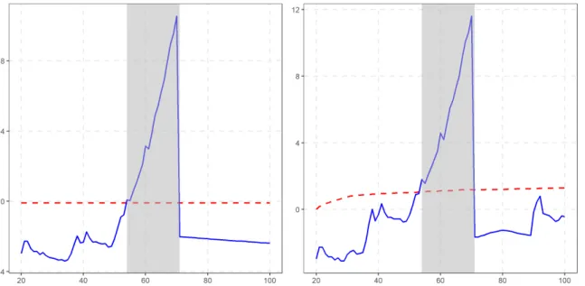
Figure 3: Datestamping with the SADF (left) and GSADF (right) tests.
A visual inspection of the two graphs in Figure 3 reveals that once the bubble starts, the BADF and BSADF test statistics gradually increase and eventually exceed their critical val-ues, rejecting the null hypothesis of no explosiveness. When the bubble bursts, both statistics fall below the critical bound almost instantaneously and remain there until the end of the sample.
To obtain the exact dates of the origination and collapse of the bubble and the bubble duration, we use thedatestamp() method.
R> datestamp(radf_sim)
Using `radf_crit` for `cv`.
Datestamp (min_duration = 0) Monte Carlo
--series1 :
Start End Duration 1 54 70 16
R> datestamp(radf_sim, option = "sadf")
Using `radf_crit` for `cv`.
Datestamp (min_duration = 0) Monte Carlo
--series1 :
Start End Duration 1 54 70 16
The results indicate that the bubble started at observation 54 and continued until observation 70. In sum, both tests perform well in detecting and dating the period of exuberance.
5.2. International House Prices
In our second application, we employ data on real house prices provided by the International House Price Database of the Federal Reserve Bank of Dallas (Macket al.2011). The dataset has a cross-sectional dimension of 23 countries and starts in the first quarter of 1975, thus allowing an international perspective on the evolution of housing markets over the last four decades. We use theihpdrpackage (Vasilopoulos 2020) to download the 2015:Q1 data release directly from theRconsole, and then usedplyr(Wickhamet al.2020) to select the columns corresponding to real house prices (rhpi), excluding the Aggregate series. Finally, we use tidyr(Wickham and Henry 2020) to pivot the data into wide format.5
R> library(dplyr) R> library(tidyr) R>
R> hprices <- ihpdr::ihpd_get(version = "1501") %>% R+ filter(country != "Aggregate") %>%
R+ select(Date, country, rhpi) %>%
R+ pivot_wider(names_from = country, values_from = rhpi) R> hprices
# A tibble: 161 x 24
Date Australia Belgium Canada Switzerland Germany Denmark Spain <date> <dbl> <dbl> <dbl> <dbl> <dbl> <dbl> <dbl> 1 1975-01-01 39.2 44.3 59.3 93.8 111. 57.4 86.2 2 1975-04-01 38.5 45.4 59.0 91.8 110. 57.6 93.0 3 1975-07-01 38.6 46.5 59.7 90.4 111. 59.1 91.5 4 1975-10-01 37.8 48.1 59.4 88.9 111. 58.1 94.7 5 1976-01-01 38.0 50.6 59.1 86.8 112. 58.4 92.9 6 1976-04-01 38.2 52.0 59.7 85.9 112. 57.3 99.6 7 1976-07-01 38.4 53.4 58.7 85.0 113. 57.3 98.5 8 1976-10-01 37.9 54.8 57.5 85.2 115. 58.6 93.7 9 1977-01-01 37.9 55.9 55.8 84.5 116. 57.5 89.6 10 1977-04-01 37.8 57.5 55.2 85.1 117. 59.3 81.2 # ... with 151 more rows, and 16 more variables: Finland <dbl>,
# France <dbl>, UK <dbl>, Ireland <dbl>, Italy <dbl>, Japan <dbl>, `S. # Korea` <dbl>, Luxembourg <dbl>, Netherlands <dbl>, Norway <dbl>, `New # Zealand` <dbl>, Sweden <dbl>, US <dbl>, `S. Africa` <dbl>,
# Croatia <dbl>, Israel <dbl>
5
The house price indexes are expressed in real terms using the personal consumption expenditure deflator of the corresponding country and have the same base year, 2005.
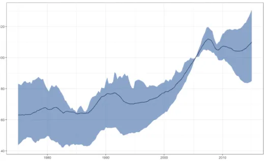
Figure 4: Real house prices.
Figure4 displays the time evolution of the cross-sectional mean of real house prices together with the lower and upper quartiles. As can be seen from the figure, mean real house prices troughed in the mid-1990s and peaked around 2006. Furthermore, by looking at the upper and lower quantiles, we observe that the run-up in real house prices during this period was not driven by the behavior of a few housing markets but it was a widespread phenomenon. This last observation has led to a consensus among economists that the latest boom-bust episode in housing played a central role in the 2008-09 financial crisis around the world, and has generated a vast interest in modeling the dynamics of house prices.
To further demonstrate the functionality ofexuber, in our econometric analysis of house prices we set the minimum window size equal to 36 quarters, the lag length equal to one, and the minimum duration of an episode of exuberance using the rule of Phillips et al.(2015a).
R> min_dur <- psy_ds(hprices) R> min_dur
[1] 5
The fact that the minimum window size differs from its default value implies that we cannot use the stored critical values to draw inference. Instead, we need to generate a newradf_cv
object. The estimation of the right-tailed unit root test statistics for all countries, and the generation of Monte Carlo critical values can be easily achieved by using the functionsradf()
andradf_mc_cv().
R> radf_hprices <- radf(hprices, minw = 36, lag = 1)
Using `Date` as index variable.
Having obtained theradf_objandradf_cvobjects, there are now a number of different ways to display the estimation results. We first focus on the presentation of country-specific results and then illustrate how the user can obtain an overall picture of exuberance for the entire dataset. Following the same approach as for the simulated data, we apply the summary(),
datestamp() and autoplot() methods to the radf_obj and radf_cv objects. The former two methods return a list of elements, with each element containing results for a specific country. For illustration purposes, we focus on the US and the UK. This choice reflects the economic size and significance of these two countries, but also the fact that their housing markets exemplify the distinct pattern of the boom-bust episode of the late 1990s and 2000s.
R> summary_results <- summary(radf_hprices, mc_critical_values) R> summary_results[c("US", "UK")] $US # A tibble: 3 x 5 name tstat `90` `95` `99` <fct> <dbl> <dbl> <dbl> <dbl> 1 adf -1.03 -0.362 0.0530 0.787 2 sadf 4.15 0.993 1.31 1.77 3 gsadf 6.04 1.55 1.78 2.39 $UK # A tibble: 3 x 5 name tstat `90` `95` `99` <fct> <dbl> <dbl> <dbl> <dbl> 1 adf -0.0907 -0.362 0.0530 0.787 2 sadf 2.94 0.993 1.31 1.77 3 gsadf 3.87 1.55 1.78 2.39
R> datestamp_results <- datestamp(radf_hprices, mc_critical_values) R> summary_results[c("US", "UK")]
$US
Start End Duration 1 1998-10-01 2007-07-01 35
$UK
Start End Duration 1 1987-07-01 1989-10-01 9 2 2000-04-01 2008-04-01 32
R> autoplot(radf_hprices, mc_critical_values, select_series = c("UK", "US"), R+ shade_opt = shade(min_dur))
Figure 5: Date-stamping periods of exuberance in the UK and US housing markets.
According to the output ofsummary(), the null hypothesis of a unit root in real house prices is rejected in favour of explosive dynamics at the 5% significance level by the SADF and GSADF tests for both the US and the UK, but not by the ADF test. Furthermore, the outputs ofautoplot() and datestamp() indicate that an episode of exuberance took place from the late 1990s/early 2000s to the late 2000s for both countries. For the UK, an episode of exuberance also took place in the first part of the sample period, from 1987 to 1989. Turning to the entire dataset, a way to concisely report first-stage results is via the function
tidy().
R> tidy(radf_hprices)
# A tibble: 23 x 4
id adf sadf gsadf <fct> <dbl> <dbl> <dbl> 1 Australia 0.502 2.82 5.47 2 Belgium -0.0410 0.996 3.16 3 Canada 0.648 0.751 4.40 4 Switzerland -2.19 2.39 3.27 5 Germany -1.22 -0.140 2.50 6 Denmark -1.02 2.00 3.01 7 Spain -1.49 0.0704 4.01 8 Finland -1.01 2.84 2.87 9 France -0.618 3.34 5.32 10 UK -0.0907 2.94 3.87 # ... with 13 more rows
# A tibble: 3 x 4
sig adf sadf gsadf <fct> <dbl> <dbl> <dbl> 1 90 -0.362 0.993 1.55 2 95 0.0530 1.31 1.78 3 99 0.787 1.77 2.39
Alternatively, one can usediagnostics()to quickly check the significance of the SADF and GSADF statistics.
R> diagnostics(radf_hprices, mc_critical_values)
Diagnostics (option = gsadf) Monte Carlo
--Australia: Rejects H0 at the 1% significance level Belgium: Rejects H0 at the 1% significance level Canada: Rejects H0 at the 1% significance level Switzerland: Rejects H0 at the 1% significance level Germany: Rejects H0 at the 1% significance level Denmark: Rejects H0 at the 1% significance level Spain: Rejects H0 at the 1% significance level Finland: Rejects H0 at the 1% significance level France: Rejects H0 at the 1% significance level UK: Rejects H0 at the 1% significance level Ireland: Rejects H0 at the 1% significance level Italy: Cannot reject H0
Japan: Rejects H0 at the 1% significance level S. Korea: Cannot reject H0
Luxembourg: Rejects H0 at the 1% significance level Netherlands: Rejects H0 at the 1% significance level Norway: Rejects H0 at the 1% significance level New Zealand: Rejects H0 at the 1% significance level Sweden: Rejects H0 at the 1% significance level US: Rejects H0 at the 1% significance level S. Africa: Rejects H0 at the 1% significance level Croatia: Rejects H0 at the 5% significance level Israel: Rejects H0 at the 10% significance level
A comparison of the results of the two econometric tests reveals large differences. For the GSADF, there is strong evidence of exuberance in real house prices with the null hypothesis of a unit root being rejected for all but three countries at the 5% significance level. On the contrary, the number of rejections of the null hypothesis is substantially smaller for the SADF test. In particular, the test cannot reject the null for almost half of the countries of our sample (13 out of the 23). Given the superior power properties of the GSADF, the conclusion that emerges is that episodes of exuberance were widespread across housing markets.
Figure6provides a chronology of the identified periods of exuberance for each country. By far, the most interesting observation is the near-simultaneous exuberance in real house prices from the early to the mid-2000s. As evident from the figure, this phenomenon has no precedent at least in our sample period, and hints to the possibility that a common factor may have contributed to house price exuberance spreading across countries.
R> autoplot(datestamp_results)
Figure 6: Date-stamping periods of exuberance in international housing markets. We explore this issue further by employing the panel recursive unit root testing procedure. This procedure requires the estimation of the panel GSADF and BSADF statistics, and the generation of the corresponding critical values. Panel test statistics are already computed as a by-product of the univariate estimation and are included in the radf objectradf_hprices. We next compute sieve bootstrap critical values withradf_sb_cv()and display the results.
R> panel_critical_values <- radf_sb_cv(hprices, minw = 36, lag = 1, seed = 145)
Using `Date` as index variable.
R> summary(radf_hprices, panel_critical_values)
Summary (minw = 36, lag = 1) Sieve Bootstrap (nboot = 500)
--panel :
# A tibble: 1 x 5
name tstat `90` `95` `99` <fct> <dbl> <dbl> <dbl> <dbl> 1 gsadf_panel 2.06 0.105 0.122 0.155
R> autoplot(radf_hprices, cv = panel_critical_values, min_duration = min_dur)
Figure 7: Date-stamping periods of overall exuberance in international housing markets.
R> datestamp(radf_hprices, panel_critical_values, min_duration = min_dur)
Datestamp (min_duration = 5) Sieve Bootstrap
--panel :
Start End Duration 1 2001-01-01 2008-10-01 31
The panel results indicate that the null hypothesis of a unit root can be rejected at all conventional levels, providing strong evidence in favor of global exuberance. Furthermore, the date-stamping results, presented in Figure 7, demonstrate in a clear manner the three phases of the international boom-bust episode in housing markets. The panel BSADF statistic sequence starts below its critical value at the beginning of the sample period; it increases rapidly after the mid-1990s and becomes significant during the early 2000s, with the period of global exuberance in housing markets continuing until 2006-07; and, finally, it collapses below its critical value.
6. Conclusion
Econometric tests of exuberance in asset prices have been attracting increasing interest over the last decade. This paper presents the R package exuber for recursive right-tailed unit root testing using the popular SADF and GSADF methodologies proposed byPhillips et al.
(2011) and Phillips et al. (2015a,b), respectively, and the panel GSADF of Pavlidis et al.
the simple and intuitive API, and its ease of use. We demonstrated these features using simulation experiments, as well as applications to artificial and real world data.
While several methodological advances have occurred over the last years, testing for and dating periods of exuberance remains a topic of ongoing econometric research. Our intention is to extend the statistical toolkit ofexuberin future versions of the package to provide users with the state-of-the-art methodologies in this area. For the near future, we plan to include the reverse-regression algorithm for detecting bubble implosion of Phillips and Shi (2018), the end-of-sample bubble detection test ofAstill, Harvey, Leybourne, and Taylor (2017), and the transmission of exuberance (contagion) test ofGreenaway-McGrevy and Phillips (2016). We also plan to incorporate the Chow-type test and the modified versions of theBusetti and Taylor(2004) and Kim(2000) tests proposed byHomm and Breitung (2012).
References
Astill S, Harvey DI, Leybourne SJ, Taylor AMR (2017). “Tests for an end-of-sample bubble in financial time series.”Econometric Reviews,36(6-9), 651–666. doi:10.1080/07474938. 2017.1307490.
Bhargava A (1986). “On the theory of testing for unit roots in observed time series.” The Review of Economic Studies,53(3), 369–384. doi:10.2307/2297634.
Blanchard OJ (1979). “Speculative bubbles, crashes and rational expectations.” Economics Letters,3(4), 387–389. doi:10.1016/0165-1765(79)90017-X.
Busetti F, Taylor AR (2004). “Tests of stationarity against a change in persistence.”Journal of Econometrics,123(1), 33–66. doi:10.1016/j.jeconom.2003.10.028.
Caspi I, Phillips PCB, Shi S (2018). psymonitor: Real Time Monitoring of Asset Markets. R package version 0.0.2, URLhttps://CRAN.R-project.org/package=psymonitor. Chang Y (2004). “Bootstrap unit root tests in panels with cross–sectional dependency.”
Journal of econometrics,120(2), 263–293. doi:10.1016/s0304-4076(03)00214-8. Eddelbuettel D (2013). Seamless R and C++ Integration with Rcpp. Springer, New York.
doi:10.1007/978-1-4614-6868-4. ISBN 978-1-4614-6867-7.
Eddelbuettel D (2019). drat: ’Drat’ R Archive Template. R package version 0.1.5, URL
https://CRAN.R-project.org/package=drat.
Eddelbuettel D, Fran¸cois R (2011). “Rcpp: Seamless R and C++ Integration.” Journal of Statistical Software, 40(8), 1–18. doi:10.18637/jss.v040.i08. URL http://www. jstatsoft.org/v40/i08/.
Eddelbuettel D, Sanderson C (2014). “RcppArmadillo: Accelerating R with high-performance C++ linear algebra.” Computational Statistics and Data Analysis, 71, 1054–1063. URL
10.1016/j.csda.2013.02.005.
Evans GW (1991). “Pitfalls in testing for explosive bubbles in asset prices.” American Eco-nomic Review,81(4), 922–930. URL https://www.jstor.org/stable/2006651.
Greenaway-McGrevy R, Grimes A, Holmes M (2019). “Two countries, sixteen cities, five thousand kilometres: How many housing markets?” Papers in Regional Science, 98(1), 353–370. doi:10.1111/pirs.12353.
Greenaway-McGrevy R, Phillips PC (2016). “Hot property in New Zealand: Empirical ev-idence of housing bubbles in the metropolitan centres.” New Zealand Economic Papers, 50(1), 88–113. doi:10.1080/00779954.2015.1065903.
Harvey DI, Leybourne SJ, Sollis R, Taylor AR (2016). “Tests for explosive financial bubbles in the presence of non-stationary volatility.” Journal of Empirical Finance, 38, 548–574.
doi:10.1016/j.jempfin.2015.09.002.
Henry L, Wickham H (2020). purrr: Functional Programming Tools. R package version 0.3.4, URLhttps://CRAN.R-project.org/package=purrr.
Homm U, Breitung J (2012). “Testing for speculative bubbles in stock markets: A comparison of alternative methods.”Journal of Financial Econometrics,10(1), 198–231.doi:10.1093/ jjfinec/nbr009.
Im KS, Pesaran MH, Shin Y (2003). “Testing for unit roots in heterogeneous panels.”Journal of econometrics,115(1), 53–74. doi:10.1016/s0304-4076(03)00092-7.
Kim JY (2000). “Detection of change in persistence of a linear time series.” Journal of Econometrics,95(1), 97–116. doi:10.1016/s0304-4076(99)00031-7.
Lacerda PAG, Phillips PC, Shi SP (2018).MultipleBubbles: Test and Detection of Explosive Behaviors for Time Series. R package version 0.2.0, URLhttps://CRAN.R-project.org/ package=MultipleBubbles.
Mack A, Mart´ınez-Garc´ıa E,et al. (2011). “A cross-country quarterly database of real house prices: a methodological note.”Globalization and Monetary Policy Institute Working Paper, 99. doi:10.24149/gwp99.
Maddala GS, Wu S (1999). “A comparative study of unit root tests with panel data and a new simple test.” Oxford Bulletin of Economics and statistics, 61(S1), 631–652. doi: 10.1111/1468-0084.0610s1631.
Mersmann O (2019). microbenchmark: Accurate Timing Functions. R package version
1.4-7, URLhttps://CRAN.R-project.org/package=microbenchmark.
Microsoft, Weston S (2020).foreach: Provides Foreach Looping Construct. R package version
1.5.0, URLhttps://CRAN.R-project.org/package=foreach.
Narayan PK, Mishra S, Sharma S, Liu R (2013). “Determinants of stock price bubbles.”
Economic Modelling,35, 661–667. doi:10.1016/j.econmod.2013.08.010.
Pavlidis EG, Mart´ınez-Garc´ıa E, Grossman V (2019). “Detecting periods of exuberance: A look at the role of aggregation with an application to house prices.” Economic Modelling, 80, 87–102. doi:10.1016/j.econmod.2018.07.021.
Pavlidis EG, Paya I, Peel DA (2017). “Testing for speculative bubbles using spot and forward prices.”International Economic Review,58(4), 1191–1226. doi:10.1111/iere.12249.
Pavlidis EG, Yusupova A, Paya I, Peel DA, Mart´ınez-Garc´ıa E, Mack A, Grossman V (2016). “Episodes of exuberance in housing markets: In search of the smoking gun.”The Journal of Real Estate Finance and Economics,53(4), 419–449. doi:10.1007/s11146-015-9531-2. Phillips PC, Shi SP (2018). “Financial bubble implosion and reverse regression.”Econometric
Theory,34(4), 705–753. doi:10.1017/S0266466617000202.
Phillips PCB, Shi S, Yu J (2015a). “Testing for multiple bubbles: Historical episodes of exuberance and collapse in the S&P 500.” International Economic Review, 56(4), 1043– 1078. doi:/10.1111/iere.12132.
Phillips PCB, Shi S, Yu J (2015b). “Testing for multiple bubbles: Limit theory of real-time detectors.”International Economic Review,56, 1079–1134. doi:10.1111/iere.12131. Phillips PCB, Wu Y, Yu J (2011). “Explosive behavior in the 1990s NASDAQ: When did
exuberance escalate asset values?” International Economic Review, 52(1), 201–226. doi: 10.1111/j.1468-2354.2010.00625.x.
R Core Team (2020). R: A Language and Environment for Statistical Computing. R Foun-dation for Statistical Computing, Vienna, Austria. URLhttps://www.R-project.org/. Sridharan S, Patel JM (2014). “Profiling R on a contemporary processor.”Proceedings of the
VLDB Endowment,8(2), 173–184. doi:10.14778/2735471.2735478.
Vasilopoulos K (2020). ihpdr: Download Data from the International House Price Database. R package version 1.2.0, URLhttps://CRAN.R-project.org/package=ihpdr.
Wang E, Cook D, Hyndman RJ (2020). “A new tidy data structure to support exploration and modeling of temporal data.”Journal of Computational and Graphical Statistics. doi: 10.1080/10618600.2019.1695624. URL10.1080/10618600.2019.1695624.
Wickham H, Fran¸cois R, Henry L, M¨uller K (2020).dplyr: A Grammar of Data Manipulation. R package version 0.8.5, URLhttps://CRAN.R-project.org/package=dplyr.
Wickham H, Henry L (2020). tidyr: Tidy Messy Data. R package version 1.0.2, URL