knowCube for MCDM –
Visual and Interactive Support for
Multicriteria Decision Making
Bericht 50 (2003)
Alle Rechte vorbehalten. Ohne ausdrückliche, schriftliche Gene h mi gung des Herausgebers ist es nicht gestattet, das Buch oder Teile daraus in irgendeiner Form durch Fotokopie, Mikrofi lm oder andere Verfahren zu reproduzieren oder in eine für Maschinen, insbesondere Daten ver ar be tungsanlagen, verwendbare Sprache zu übertragen. Dasselbe gilt für das Recht der öffentlichen Wiedergabe.
Warennamen werden ohne Gewährleistung der freien Verwendbarkeit benutzt.
Die Veröffentlichungen in der Berichtsreihe des Fraunhofer ITWM können bezogen werden über:
Fraunhofer-Institut für Techno- und Wirtschaftsmathematik ITWM Gottlieb-Daimler-Straße, Geb. 49 67663 Kaiserslautern Telefon: +49 (0) 6 31/2 05-32 42 Telefax: +49 (0) 6 31/2 05-41 39 E-Mail: [email protected] Internet: www.itwm.fraunhofer.de
Das Tätigkeitsfeld des Fraunhofer Instituts für Techno- und Wirt schafts ma the ma tik
ITWM um fasst an wen dungs na he Grund la gen for schung, angewandte For schung
so wie Be ra tung und kun den spe zi fi sche Lö sun gen auf allen Gebieten, die für
no- und Wirt schafts ma the ma tik be deut sam sind.
In der Reihe »Berichte des Fraunhofer ITWM« soll die Arbeit des Instituts kon ti
nu ier lich ei ner interessierten Öf fent lich keit in Industrie, Wirtschaft und Wis sen
-schaft vor ge stellt werden. Durch die enge Verzahnung mit dem Fachbereich
the ma tik der Uni ver si tät Kaiserslautern sowie durch zahlreiche Kooperationen mit
in ter na ti o na len Institutionen und Hochschulen in den Bereichen Ausbildung und
For schung ist ein gro ßes Potenzial für Forschungsberichte vorhanden. In die
richt rei he sollen so wohl hervorragende Di plom und Projektarbeiten und Dis ser
-ta ti o nen als auch For schungs be rich te der Institutsmi-tarbeiter und In s ti tuts gäs te zu
ak tu el len Fragen der Techno- und Wirtschaftsmathematik auf ge nom men werden.
Darüberhinaus bietet die Reihe ein Forum für die Berichterstattung über die
rei chen Ko o pe ra ti ons pro jek te des Instituts mit Partnern aus Industrie und
schaft.
Berichterstattung heißt hier Dokumentation darüber, wie aktuelle Er geb nis se aus
mathematischer For schungs- und Entwicklungsarbeit in industrielle An wen dun gen
und Softwareprodukte transferiert wer den, und wie umgekehrt Probleme der
xis neue interessante mathematische Fragestellungen ge ne rie ren.
Prof. Dr. Dieter Prätzel-Wolters
Institutsleiter
Support for Multicriteria Decision Making
Hans L. Trinkaus
∗, Thomas Hanne
Fraunhofer Institute for Industrial Mathematics (ITWM)
Department of Optimization
Gottlieb-Daimler-Str. 49
67633 Kaiserslautern
Germany
e-mail: [email protected], [email protected]
Abstract
In this paper, we present a novel multicriteria decision support
sys-tem (MCDSS), called
knowCube
, consisting of components for knowledge
organization, generation, and navigation. Knowledge organization rests
upon a database for managing qualitative and quantitative criteria,
to-gether with add-on information. Knowledge generation serves filling the
database via e.g. identification, optimization, classification or simulation.
For “finding needles in haycocks”, the knowledge navigation component
supports graphical database retrieval and interactive, goal-oriented
prob-lem solving.
Navigation “helpers” are, for instance, cascading criteria
aggregations, modifiable metrics, ergonomic interfaces, and customizable
visualizations. Examples from real-life projects, e.g. in industrial
engi-neering and in the life sciences, illustrate the application of our MCDSS.
Key words:
Multicriteria decision making, knowledge management, decision
support systems, visual interfaces, interactive navigation, real-life applications.
1
Introduction
Usually, real-life decision problems are characterized by several criteria or
objec-tives to be taken into consideration. Despite the fact that “multiple objecobjec-tives
are all around us”, as Zeleny (1982) points out, the dissemination of methods
for multicriteria decision making (MCDM) into practice can still be regarded
∗Corresponding author
as insufficient. A basic reason for that situation might be that practitioners are
just not familiar with MCDM methods, which often are difficult to understand
and to work at. One main difficulty for an easy and explorative usage of
meth-ods might be caused by the user interface, i.e. the handling of interactions with
a corresponding computer program. Zionts (1999) is pointing out the necessity
of user-friendly software in the following way: “I strongly believe that what is
needed is a spreadsheet type of method that will allow ordinary people to use
MCDM methods for ordinary decisions.”
In this paper, we present a novel multicriteria decision support system
(MCDSS), called
knowCube
, which mainly originates from focussing on
user-specific needs.
Therefore, the first aspect of the system is the provision of
visualizations and interactivity in categories well understandable by non-expert
users. All technical stuff, necessary for this comfortable presentation of and
access on knowledge, is hidden in the background, combined in a so-called
navi-gation component. Its integration with further components, for generating and
managing knowledge data required for decision processes, is another main
fea-ture of this MCDSS.
The paper is organized as follows: Section 2 introduces some notation for
multicriteria decision problems. (Here we restrict ourselves to tasks dealing
only with quantitative criteria, other types of criteria will be topics of a
pa-per to follow.) In Section 3, we present a survey of components of
knowCube
,
and additionally some details on the generation and organization of decision
knowledge. MCDM-specifics of
knowCube
, including a short excursion to
hu-man cognition, are discussed in Section 4. Two examples show the application
of
knowCube
in real-life projects, one in the field of industrial engineering
(Sec-tion 5), another one in medical radia(Sec-tion therapy (Sec(Sec-tion 6). The paper ends
with some conclusions and an outlook to future work (Section 7),
acknowledge-ments and references (Sections 8 and 9), and an appendix (Section10), meant
to convince the “sceptical” reader of some ideas presented in the paper.
2
Multicriteria Decision Problems
In the following we assume multicriteria decision problems
(
A, f
)
defined by a feasible set of alternatives
A
and a vector-valued (
q
dimensional)
objective function
f
= (
f
1, ..., f
q)
.
For an alternative
a
∈
A
,
f
j(
a
)
, j
∈ {
1
, ..., q
}
,
represents the evaluation of
the
j
th objective (also called criterion or attribute). Each objective function
f
jis assumed to be either maximized:
max
a∈Af
j(
a
), or minimized:
min
a∈Af
j(
a
).
If
A
is a finite set, i.e.
A
=
{
a
1, ..., a
r}
,
we also use the concise notation
z
ij=
f
j(
a
i)
for denoting the
j
th criterion value for alternative
a
i. Here,
Z
= (
z
ij)
i=1..r,j=1..qis also denoted as decision matrix. In other cases,
A
may be a subset of a vector
space,
A
⊂
R
n, defined by a vector-valued restriction function
g
:
R
n→
R
m:
A
=
{
x
∈
R
n:
g
(
x
)
≤
0
}
.
In practice, such a problem may be rather complex. For instance,
restric-tions defining the feasible set may be given by analytic formulas or differential
equations.
Usually, there does not exist a solution which optimizes all
q
objectives at
the same time. Therefore, from a mathematical point of view, one may consider
the set of efficient or Pareto-optimal solutions as results to the above problem.
For two solutions
a, b
∈
A
, we say that
a
dominates
b
, if
f
(
a
)
=
f
(
b
) and
f
j(
a
)
≥
f
j(
b
)
,
if
f
jis to be maximized,
f
j(
a
)
≤
f
j(
b
)
,
if
f
jis to be minimized,
for each
j
∈ {
1
, ..., q
}
. The efficient set is then defined by
E
(
A, f
) :=
{
a
∈
A
:
∃
b
∈
A
:
b
dominates
a
}
.
Since this efficient set normally contains too many solutions, its computation
does not really solve the multicriteria decision problem from a practical point of
view – because a decision maker usually wants to get a single “good” solution,
e.g. by choosing one from an easily to survey set of meaningful alternatives.
For that purpose, an enormous number of methods for practically solving
multicriteria decision problems has been developed in the meantime. Overviews
and details referring to this are given, for instance, in Hanne (2001), Steuer
(1986), Vincke (1992), or Zeleny (1982).
One idea for example, common to some of these solution approaches, is to
use additional preference-related information (stated by the decision maker) on
the multicriteria problem, which then may result in obtaining a single solution.
Popular concepts of these methods are taking specific values of the objectives
(which may or may not correspond to feasible solutions) to compare solutions
with. The earliest technique in MCDM using a desired solution (“the goal”) and
minimizing the alternatives’ distance to it is goal programming, developed as
an extension of linear programming. Today, there are many new methods which
utilize various kinds of desired and undesired solutions, different metrics, and
additional features. Usually, these methods are called reference point approaches
(Wierzbicki (1998)).
In absence of user-specified reference points, the following two concepts are
frequently used: The utopia (or ideal) point
u
is defined by the component-wise
best values of the alternatives in objective space, i.e.
u
j=
max
a∈Af
j(
a
)
,
if
f
jis to be maximized,
min
a∈Af
j(
a
)
,
if
f
jis to be minimized,
for
j
∈ {
1
, ..., q
}
.
The nadir (or anti-utopia) point
v
is defined by the
component-wise worst values, but considering only efficient alternatives, i.e.
v
j=
min
a∈E(A,f)f
j(
a
)
,
if
f
jis to be maximized,
max
a∈E(A,f)f
j(
a
)
,
if
f
jis to be minimized,
for
j
∈ {
1
, ..., q
}
.
Based on Simon’s (1957) theory of satisfying, which was developed as an
alternative to utility maximization, concepts using aspiration and reservation
levels (or thresholds) became popular in multicriteria decision making.
Tak-ing aspiration levels for MCDM has first been pointed out by Tversky (1972a,
1972b). His approach of a successive elimination by aspects, is based on the
idea that human decision making frequently works as a stochastic process for
exploring alternatives. By choosing minimum requirements for the outcomes
in specific criteria, the decision space
A
is reduced while the decision maker
learns more about the feasible alternatives. Some features of the navigation
process described below in this paper may be considered as an extension and
user-friendly implementation of Tversky’s basic concepts.
Considering the limited capabilities of real-life decision makers, nowadays
there is a significant number of methods providing ergonomic interactivity and
means for visualization. Some of these are, for instance, described in Belton and
Vickers (1993), Korhonen (1987, 1988), Korhonen and Laakso (1986a, 1986b),
Korhonen and Wallenius (1988).
A specific visualization technique used in our MCDSS, is called radar chart,
spider web or spider chart. It is based on the idea of representing several axes in a
star-shaped fashion. An object characterized by multiple attributes then may be
represented in the diagram as a polygon, resulting from connecting lines between
the attribute scores on neighboring axes. Although such kinds of diagrams are
rather common in statistics and brainstorming techniques, only few MCDM
methods so far utilize this approach. And – there are some additional new
features in our MCDSS, as for example the fact, that the polygon representing
an alternative by its objective values as corner points “has got life”: Online
mouse-manipulations on the screen enable an interactive navigation through
the database of decision alternatives.
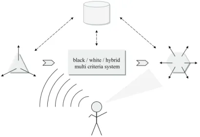
By talking so much about visualization, it should be appropriate just to do
this – as the sketch shown in Figure 1 perfectly illustrates the scope of
knowCube
:
A decision maker, comfortably interacting (by ear, eye, mouth, or hand) with
an MCDSS!
black / white / hybrid multi criteria system
Figure 1: “One picture means more than thousand words.”
More explanations and especially practical details will be given in the next
sections, here we only want to look still somewhat closer on the core of the
multicriteria decision task, where we distinguish the following cases: If the
description of the problem is known and completely given, it is called a “white”
(box) multicriteria problem. This is the case mostly assumed in multicriteria
optimization methods, applied for finding “the best of all possible solutions”.
If nothing is known about structure of or dependencies within the multicriteria
problem, it is denoted as “black”. Typically, outcomes of such systems are,
for example, found by trial and error, or won by general inquiries. Frequently,
such results are not reproducible, and in many cases all results are evolving in
the sense that the problem settings are changing with time. Most real decision
situations however are somewhere in between “black and white”, which lead
to “hybrid” multicriteria problems. Then carrying out costly experiments and
importing the results obtained into the database are the means chosen very
often. But also simulation methods gain in increasing significance for getting
decision suggestions.
As already indicated in Section 1, here we are considering only quantitative
criteria variables – to keep it simple, to introduce the main concepts of
knowCube
,
as a first step, and to have place for explaining the basics by examples. For
work-ing with other types of criteria – like qualitative, objective/subjective,
ratio-nal/irrational, active/passive, dependent/independent, deterministic/statistic,
hard/soft, timely, ..., and all mixed together – the topics introduced so far must
be slightly extended. This will happen in a paper to follow.
3
Scope of
knowCube
, Knowledge Organization
and Knowledge Generation
knowCube
, seen as a general framework of an MCDSS, consists of three main
components:
knowOrg, knowGen,
and
knowNav
(knowledge organization,
gen-eration, and navigation). These are put together with their sub modules into a
common box, showing to various decision makers varied views – like the different
faces of a cube. This gives a hint at the term “knowledge cube”, abbreviated
knowCube
, taken as a “logo” for the complete MCDSS. Figure 2 illustrates its
structure.
knowCube knowOrg knowBlo knowBas knowMet knowSto knowGen knowOpt knowExp knowSim knowImp knowNav knowVis knowSel knowDisFigure 2: The Structure of
knowCube
.
The “bricks” shown there may act self-contained up to a certain extent, but
they also are designed for efficient interaction in the configuration of special
“buildings” for specific needs. So
knowCube
is customizable for use as a decision
support system in various application domains. This will become more evident
in Sections 5 and 6, where two examples are presented, one in the field of
industrial engineering, another one from among medical applications.
For an easy integration of
knowCube
into an institution’s workflow, the
com-ponent
knowOrg
provides comfortable tools for data collection, recording,
admin-istration, and maintenance – and all that with comparatively little effort. Open
data interfaces enable information exchange with external data sources, such
that the database of
knowCube
may be extended by arbitrary “external”, and
also “historic”, decision support information. These topics mainly are handled
by the modules
knowBas
(knowledge base) and
knowSto
(knowledge storage).
(More details will be worked out in a future paper.)
Making decisions presupposes some knowledge. So, in any case, a data base
must be filled with decision information, where its fundamental unit is called
knowBlo
(knowledge block). Such a block consists of two parts, one containing
all those criteria values corresponding to a specific decision alternative (e.g.
a row of the decision matrix
Z
, in case of a finite set of alternatives
A
), the
other one references to additional information attachments. Those may be,
for instance, documents, diagrams, graphics, videos, audios, ..., any media are
allowed. The usage of criteria and attachment information is best explained
within application contexts, which will be shown later in the examples already
mentioned.
The last “brick” in the
knowOrg
component to talk about is
knowMet
(knowl-edge metric). Here, the singular of the word “metric” is a bit misleading: There
is not only one metric or one class of similar metrics defined on the data base,
but additionally a big family of metric like orderings. For instance, all
l
pmetrics
(1
≤
p
≤ ∞
) may be used, at least for quantitative criteria blocks, together with
superimposed priority rankings – which furthermore are “online user adaptive”.
Besides that, certain filtering functions allow some clusterings and inclusions or
exclusions of sets of data blocks.
So far for the first component of
knowCube
, corresponding to the data base
symbol on the top in the sketch of Figure 1. There the dotted lines indicate,
that the decision maker usually does not take care about these interrelations,
they must act silently on the back stage.
An engaged decision maker or, at least, the decision provider and analyst will
show more interest in the second component
knowGen
(knowledge generation),
which comprises the framework for producing decision information to fill the
data base for a given multicriteria problem. Thereby, the main tasks are to
formulate and answer questions such as e.g.:
•
What kind of system will model the decision situation?
•
Which criteria are identifiable?
•
How may the criteria variables be arranged in groups?
•
Could information be aggregated following a top-down approach?
•
Which add-on media should be attached for supporting decision processes?
After these “preliminaries” the interfaces between the acute knowledge
gen-eration domain and the components
knowOrg
and
knowNav
are adjusted. Then,
one or more of the following activities may be started, corresponding to the
“bricks” of
knowGen
in Figure 2:
•
Optimization calculations (in the “white system” case) – delivering e.g.
Pareto solutions as outcomes of the module
knowOpt
(knowledge
optimiza-tion).
•
Performing experiments (in the “hybrid system” case) – observing results,
e.g. from optimal experimental design methods, as produced by
knowExp
(knowledge experiments).
•
Doing simulations (again in the “hybrid system” case) – getting e.g. data
records with a mixture of some hard/soft criteria, where the input and
output values are generated by some standard simulation software tools,
gathered in
knowSim
(knowledge simulation).
•
Collecting data “events” (in the “black system” case) – e.g. by reading
information from external sources via
knowImp
(knowledge import).
•
Using some other problem specific method – which is not discussed above,
and indicated in Figure 2 by dotted lines.
In any case, the modules
knowMet
and
knowSto
are closely working together,
if some newly generated or acquired decision knowledge (
knowBlo
) is put into
the data base (
knowBas
). The data base filling processes may be organized via
batch procedures, interactively, and also in an evolving way, i.e. within several
time slots and under various external conditions – exactly as in real life, and
also with the well known effect that “old” decisions are overtaken by “new”
ones.
As illustrated in Figure 1, knowledge generation happens mainly in the center
of
knowCube
. So for example, by feeding or controlling the
black/white/hybrid-system (possibly also by acoustic commands), and by receiving or observing
corresponding system answers.
A more distinct explanation of so far introduced concepts will be given below,
especially in context with the two already mentioned application examples –
after a short break:
4
About Visual Data Processing and Human
Cognition – Towards
knowCube
Navigation
Some simple tests (as given by the Appendix in Section 10) and thereof
de-rived conclusions will motivate the design and functionalities of the visual
inter-face of
knowCube
in general, and especially the ideas of the so-called
knowCube
Navigator
.
Let us summarize some basic principles of visual data processing – which
are well known long ago, and may be found e.g. in Cognitive Psychology by
Wickelgren (1979) – by three statements:
Statement 1:
Reading text information or listening to a speaker is not
sufficient to generate knowledge for solving problems or making decisions!
Statement 2:
The human visual system has a highly efficient information
processing architecture. It allows inferences to be drawn based on visual spatial
relationships – fast and with small demands on “working space capacity”!
Statement 3:
The human visual system is also highly sensitive for moving
objects and changing shapes!
Quintessence:
Supporting decision making should appeal to the human
visual system, transforming complex situations into time-animated, spatial
pre-sentations!
So, visual spatial relationships, moving objects and changing shapes – all
these general topics should be integrated in a tool for supporting decision
mak-ing, at the least. But, additionally to that, such a tool asks for some more
specific and practical demands on its man/machine interface. These
require-ments, gained by experience and evaluated by experirequire-ments, will be formulated
in the sequel as axioms, and visualized by easy examples.
The first step in the process of optical perception is the division of a
“pic-ture” into a “figure”, which comes by a filtering process to consciousness, and
into the “background”, which is no longer of interest. The main question for
designing visual interfaces based on “figures” is: What are the main principles
for recognizing figures out of arbitrary forms?
Many of the answers given below as axioms already have been discovered
during the development of Gestalt Psychology, as a theory of perception by
Wertheimer (1923) and others, during the 1910s and 20s. Nowadays, these
ideas are common knowledge, and extensively used in multimedia applications;
cf. Macromedia Director 7 (2000).
Axiom 1: Closedness.
The most elementary forms that are interpreted
as figures are surrounded by closed curves.
Axiom 2: Closeness.
Objects close together are seen as figures, distant
objects are assigned to the background.
An example is given in Figure 3. Each sketch contains eight domains, which
are all closed. But they are hardly perceived all at the same time. The sketch
on the left shows a cross standing upright, on the right it is inclined. Narrow
parts are taken together as the arms of the crosses, broader parts within the
sketches are seen as interspaces or background. (Only with a certain effort it is
possible to discover an upright cross with broad arms in the sketch on the right,
too.)
Figure 3: Picture, Figure and Background.
Now knowing the two basic principles of “identifying” figures: closedness
and closeness, the question arises: Which principle dominates?
Axiom 3: Closedness versus closeness.
If closedness and closeness are
competing, it’s more likely that closed forms are taken as the figures looked for.
Figure 4 should convince us: Broader domains become figures, because they
are closed. The narrow sectors no longer appear as arms of a cross, since little
parts of their boundaries are missing.
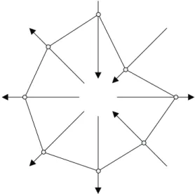
Finally, to get closer to our goal: the
knowCube Navigator
, we present as a
last concept needed:
Axiom 4: Convexity.
All convex forms – or roughly convex forms as e.g.
star-like shapes – are particularly easy recognized as figures.
This was already realized by v. Hornbostel (1922). Here is an example:
Figure 5: Star-like Shape – or ”Nearly Convexity”.
Though not looking quite nice, the polygon bounding a nearly convex domain
is eye-catching. The line segments, oriented radially towards a common invisible
center, are obtaining less attention. This contrast will still increase, if “the
line segments stay at rest, and the polygon starts to move”. Such a
poly-gonal representation is the most central visualization tool of
knowCube
’s main
component
knowNav
, which provides the core navigation tools.
So, we are getting closer now towards
knowCube
navigation:
Each variable is related to a line segment, the line segments are arranged like
a “glory”, each segment shows a scale (linear or something else), where small
values always are put towards the center to avoid confusion. Each segment gets
an arrow-head pointing towards that direction (bigger or smaller values), which
is preferred by the decision maker for the corresponding criterion.
Little circles on the segments represent the current parameter values of a data
base record – or decision alternative, respectively. Adjacent circles are connected
by straight lines, all together defining a closed polygon, which bounds a convex
or at least star-shaped region. By this little trick the observer or decision maker
comprehends “what belongs together”.
Summing all up: A closed polygon within a star-shaped scale arrangement
visualizes a record in the data base
knowBas
.
Three of them are to be minimized, the other ones are to be maximized. (For
the sake of simplicity, the scales on the segments are omitted here – but they
are shown in the second application example in Section 6.) The order of the
criteria’s arrangement may, for instance, reflect their importance, or it may be
chosen interactively according to the user’s preferences.
Figure 6: A Decision Alternative, Represented in
knowCube
.
To the end (of this Section) two questions still are open: How are
informa-tion attachments supporting the decision making? What about the dynamic
behavior of polygons?
Best answers will be given by two already announced real-life applications:
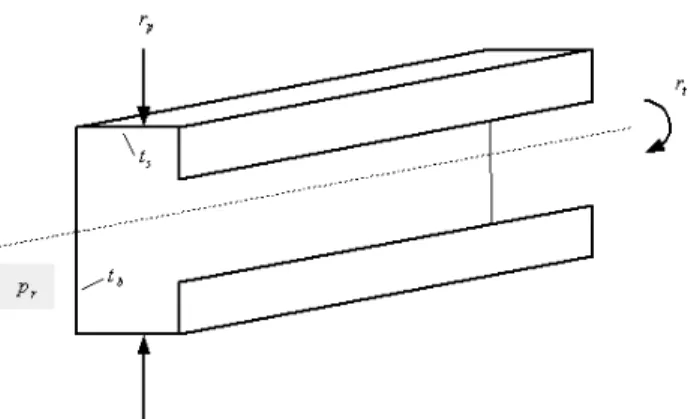
5
Designing “Best” Trunking Devices
We consider the industrial engineering problem of designing the profile of a
new electrical trunking device – that is usually fixed at the wall, and used for
a comfortable laying of multitudes of cables. The problem is to find a best
cross-section profile for such trunking devices.
Many objectives are to be taken into account in such a development process.
Among them there is one group of criteria, which should be minimized:
a
m,
the total amount of material needed for one unit of the trunking device;
t
p,
the time to produce one unit;
c
u, the overall cost for one unit. For a better
understanding of a second group of variables, Figure 7 will help, showing in
front the approximately U-shaped cross-section of a trunking device.
r
ppoints
to the resistance of the trunking device against pressing from opposite sides,
r
tto its resistance against torsion. These two variables should have big values, of
course.
Figure 7: A Trunking Device.
The five criteria introduced so far may be considered as characterizing the
outcome of a specific design for a trunking device. Their resulting values
obvi-ously are caused by a third group of (in a certain sense “independent”) variables:
t
bdenotes the thickness of the bottom face,
t
sthe thickness of the side face of
the device. A last variable
p
r(not visualized, but only mentioned in Figure 7)
specifies the portion of recycling material, used e.g. for producing PVC trunking
devices. All these eight variables are “working together”, in nontrivial, highly
nonlinear, and partially conflicting combinations.
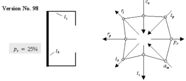
Assuming now, that the engineering team has designed plenty of different
profile versions, evaluated them virtually (e.g. by some finite element methods
out of
knowSim
), according to the above criteria (which correspond to
f
1, ..., f
8,
as introduced in Section 2), and put all together with some operational data into
the data base, then some data blocks could be presented as shown in Figures
8-10.
Figure 9: Design Alternative 98.
Figure 10: Design Alternative 746.
With the generation of these data, the job of the engineering team is done.
Now the time has come for the management of the enterprise to decide which
new type of trunking devices is going to be launched. But, of course, a top
manager would not want to look over hundreds of data sheets.
Here the
knowCube Navigator
supports the user to “stroll” easily, quickly,
and goal oriented through the data base. By pulling at a vertex of the
naviga-tion polygon, at a so-called grip point, towards smaller or larger values (inwards
or outwards), the polygon moves or transforms to a neighboring polygon,
rep-resenting another element of the data base.
In the background the module
knowMet
is looking online for that “new”
data record, which in the first place is different but closest to the “old” one,
with respect to the criterion that was gripped, and which in the second place is
“closest” to the “old” record, with respect to all other criteria.
It certainly would be an essential advantage for the top manager always to
know “where he/she is”, and which goals are achievable in the best case. An
additional graphical assistance will help here:
For each criterion there are taken the respective values from all records in the
data base. Virtually, the resulting point set is plotted on the corresponding line
segment. The smallest interval containing such a set defines a decision range
of potential alternatives for that specific criterion. Then connecting “inner”
(neighboring) interval endpoints by straight lines determines the inner
deci-sion boundary, the outer decideci-sion boundary results by analogy. Both together
“construct” the decision horizon. The metaphor “horizon” is used, because the
decision maker knows and “sees” in advance that each possible alternative,
re-spectively selection of a data record or corresponding polygon representation,
will lie somewhere within this area – that is emphasized in the sketch in Figure
11 by some color shading. (The utopia point
u
, mentioned in Section 2,
corre-sponds to that polygon, which connects those boundary points of the shaded
area, lying on the variables’ line segments and closest to their arrow heads. The
nadir point
v
results vice versa.)
Figure 11: “What Is Achievable – What Not?”.
By the way, the decision horizon serves as an ideal base for discussions at
meetings, where many decision makers are fighting with plenty, usually
conflict-ing, arguments. Acute viewpoints may be ranged in easily by the “location”
of the navigation polygon, extreme positions may be estimated by the inner
and outer boundaries. Alternatives, their pros and cons, are visualized
interac-tively. The attachment knowledge, as e.g. the sketches of the cross sections in
Figures 8-10 or the visualizations in Figure 12, helps to get to more objective
conclusions.
Furthermore, there are some additional tools for facilitating the process of
decision making:
•
Locking parts of decision ranges.
Some criteria values may not be acceptable in any way, already from
the beginning of the “decision session”. Some other criteria values may
no longer be of interest, after exploring and discussing a certain amount
of alternatives. In any case, locking subintervals on the decision ranges
(e.g.
via clicking on it with the mouse and pulling along the criteria
segment) leads to a restricted decision horizon, corresponding records in
the database are set inactive. Unlocking of locked parts is possible at any
time, of course. By such a process of consecutive lockings and unlockings,
a decision maker may find within the decision horizon his/her own decision
corridor, enclosing only those candidates being of interest furthermore –
while the rest is put into the background.
•
Logging navigation paths.
Everybody has experienced, that a situation of the past seemed to be
“better” than a present one – but the way how to get to that place has
been forgotten. To avoid such problems, there is written automatically a
log-file, memorizing all steps of the navigation path walked so far.
Walk-ing through this log-file then may be done by usWalk-ing interactive recorder
buttons with their well-known functionalities.
•
Storing and viewing “good” alternatives.
The decision maker may memorize every alternative evaluated positively
by a store button, writing the corresponding reference into a memo-file.
This file specifically may be used at presentations, e.g. for visualizing
the process of coming to a certain final decision. Here the successive
al-ternatives may be combined and animated as a “movie”. Each singular
“picture” consists of a snapshot of the acute navigation polygon, together
with (user dependent, selectable) attached information. The changes
be-tween the pictures are done by slow cross-fadings, a technique that fits
well to the human cognitive system.
•
Clustering decision alternatives.
Combining the functionalities described above allows to construct
cluster-ings within the data base interactively. Starting with a chosen alternative,
e.g. by means of the view-button, and then using two-sided lockings
suc-cessively on each decision range, constructs a temporary inner and outer
boundary. All navigation polygons lying within define a cluster – by the
way, pointing to a new way for visualizing clusters and their centers.
All tools described above may be used by the top management, that has to
decide, which design version of profiles should be produced by the company in
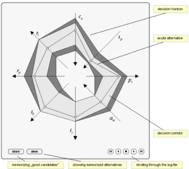
future. Figure 12 shows some parts of the navigator’s graphical user interface
for this specific example. Several steps (e.g. locking) in the decision process
already have taken place, the acute alternative is represented by the polygon
lying within the lightly shaded corridor.
Figure 12: knowCube Navigator.
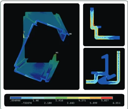
Popup-windows serve to show attached information, as for instance in
Fig-ure 13, the (exaggerated) torsion under a certain force (big pictFig-ure), and the
material stress visualized by colorings of distinguished profile details (small
pic-tures).
Now, a last time back to the visualization of the “vision” in Figure 1: The
knowCube Navigator
supports the decision maker (easily identified at the
bot-tom of the sketch) by offering to him/her a number of decision horizons, which
are organized corresponding to the specific needs of the concrete application.
So, in some cases, one horizon could contain only dependent criteria, and the
decision maker were examining the outcomes, as shown on the right side of the
sketch. Another horizon could handle independent criteria, and the decision
maker were working with these, like on the left side of the sketch, e.g. also
by acoustic or even tactile interaction, what could make sense especially for
handicapped persons.
Figure 13: Design of Trunking Devices – Information Attachment.
For further illustration of the manifold applicability of
knowCube
and its
Navigator
, another real-life case will be presented, belonging to a completely
different domain, and which is – not only from a mathematical point of view –
much more complex than the technical design task just discussed. This medical
application illustrates the “power” of
knowCube
very well. It is especially a
well-fitting instance for demonstrating parallel utilization and visualization of
hierarchically aggregated attachment information in a transparent way.
6
An Interactive Decision Support System for
Intensity Modulated Radiation Therapy
“What is the ideal radiation therapy plan for a patient?”
Within the complete, time consuming workflow process of intensity
modu-lated radiation therapy (IMRT), two topics are of main interest for the
opti-mization task: First, the segmentation of the CT (computer tomography) or
MR (magnetic resonance) slides, i.e. adding curves onto the slides, describing
the boundaries of the tumor and the
R
organs at risk – which in most cases
must be done manually, at least today. Second, the dose calculation, i.e.
com-puting the dose contributions to each voxel (volume element inside the body) of
interest, coming from corresponding bixels at the beamheads (beamhead pixels)
of a linear accelerator, used for the radiation treatment.
Some output of these two steps is taken as input for the knowledge data
base: General information concerning the patient to be treated, his/her CT or
MR slides, the segmentation contours, and the dose matrix.
A slide is a 256 x 256 or 512 x 512 grey-value pixel image, and because up
to 40 parallel slides in 3 different orientations – transversal, frontal, sagittal –
are needed, CT or MR slides means “fat data”. The same holds for the dose
matrix, up to one million entries are not unusual. Segmentation contours, on
the other hand, means “slim data”, that takes merely some kB.
Now the optimization procedure, done within the module
knowOpt
, may
start, taking about four hours on a high-end PC. It generates up to 1000
dis-tinct Pareto optimal 3D-solutions, “covering” the planning horizon with a grid
of planning alternatives for the patient. In this specific case, a solution assigns
a real number to each bixel, representing the amount of radiation emitted from
there. The superposition of all bixel contributions sums up to a radiation
distri-bution in the volume of interest, containing the tumor and neighboring organs
at risk. Each of these objects obtains a set of “notes” – as e.g. numbers,
func-tions, and point sets – by which the decision maker will be able to estimate
their “qualities”. More details on radiation therapy planning are presented in
Bortfeld (1995), and Hamacher and K¨
ufer (1999).
All calculations mentioned above happen automatically, they may be done
overnight as a batch job, and stored in the data base
knowBas
. The next day,
the results may be transferred to a notebook, such that the physician (and even
his/her patient) may look for the optimal plan interactively.
But then – how to manage this enormous quantity of data to find out the
“best” plan with reasonable effort?
This works
•
by real-time accesses on the pre-calculated and pre-processed data base
mentioned above – which in particular contains various data aggregations
in a cascading manner,
•
by simultaneous visualizations of dose distributions – in the shape of well
known (for a physician, at least) dose-volume-histograms and colored
iso-dose lines (“slim data”), superimposed on the patient’s grey-value CTs or
MRs (“fat data”), and, on top of that,
•
by our tricky exploration tool
knowCube Navigator
, which supports and
controls the interactive, goal oriented tour through the huge variety of
planning solutions – leading towards the patient’s optimal radiation
ther-apy plan within some minutes.
Some details will be explained now by a typical navigation session:
The physician starts the program, types in his/her identification and the
patient’s name, and gets a planning screen, which contains some information
objects similar to Figure 14.
Figure 14: GUI for IMRT.
One part of the graphical user interface (GUI) shows static information,
concerning the patient of interest and the physical setup, that was given – or
selected, e.g. from a data base – before the optimization computations were
started. The other parts of the GUI contain dynamic information: With the
beginning of the planning session, the main pointer of the database references
on the solution of least common tolerance – a kind of “average solution”, that
balances “notes” of conflicting criteria.
Information objects, corresponding to the respective, acute solution, are
presented by the GUI in a decreasing degree of fineness:
•
“Richest” information is given by CTs or MRs, through the isocenter of
the tumor (transversal, frontal, and sagittal), superimposed by in advance
calculated isolines. (Of course, it is possible to skim through these three
stacks of slides, continually getting the immediate isolines, and so gaining
maximum detail knowledge.)
•
“Medium” information content is aggregated in the dose-volume
his-togram, where each curve shows the accumulated Gray contribution per
organ at risk or tumor. (Gray is the physical unit for radiation energy.)
•
The “coarsest” information is delivered by the navigation object of the
GUI: All radiation energy absorbed by an organ at risk – or by the tumor
– is summarized in just one number, thus getting
R
+ 1 numbers (
R
risks, as already mentioned before) specifying the radiation plan. These
numbers are inscribed as pull points (i.e. grip points) on the organs’ or
tumor’s acceptance intervals (i.e. decision ranges), that are arranged in
a star-shaped sketch. Linking these grip points by line segments results
in a solution polygon (i.e. navigation polygon), characterizing the whole
planning solution from a top point of view, well-suited for a first, quick
estimate of the solution’s relevance.
To recapitulate: The starting point, the so-called solution of least common
tolerance, is visualized by various graphical objects, culminating in its solution
polygon.
But
knowCube
yields much more – and for that reason again let us look
somewhat closer on the details:
Each precalculated solution, that has been accepted to be a member of the
data base, provides for each risk, respectively for the tumor, an entry on the
cor-responding acceptance interval. So all solutions together define the ranges of the
acceptance intervals. Connecting their smallest respectively largest endpoints
delimits the shaded area, called planning horizon (i.e. decision range).
Why? It permits at any time an overview on all solutions in the data base.
The physician not only gets a general view of a solution visualized by its polygon,
but he/she also may estimate its significance with respect to all other solutions,
recognizing which planning goals really are achievable and which are not.
So now the action may start with the solution of least common tolerance:
The physician e.g. wants to reduce the total radiation given to a certain risk.
To achieve this, he/she clicks with the mouse on the corresponding pull point
and moves it towards smaller Gray values. The data base, with an index family
for modified lexicographic ordering strategies, is scanned simultaneously, such
that isolines and dose-volume curves of “neighboring solutions” are updated on
the screen at the same time. As soon as the mouse-click is released, the “moving
polygon” stops in its new position.
This first kind of action: pull, may be repeated again and again to explore
the planning horizon – with the same organ at risk or any other, and with the
tumor too, of course. Just one remark to keep an eye on: Moving a pull point
towards smaller/higher risk/tumor values results in a new solution-polygon,
where at least one other pull point shows a higher/smaller risk/tumor value –
in accordance with the Pareto optimality of the data base.
In the meantime the physician may have found a solution fulfilling his/her
first priority, e.g. a total Gray value for a specified risk that is less than a fixed
amount. Only solutions which are not worse with respect to this are of interest
furthermore. Therefore, the second kind of action: lock, is getting importance.
The physician clicks in the corresponding lock box, and the planning horizon
immediately is divided into two parts (shaded differently), a locked area and an
active area. Now active navigation is restricted – a filter selects the accessible
objects in the data base.
It should be superfluous to mention, that this locking action naturally may
be applied to more than one acceptance interval, and that unlocking, pulling,
and any combination of them is possible as well.
Some more actions are integrated in the software to facilitate the work of
the physician: storing of favored solutions, viewing of stored solutions, and
skimming through already regarded solutions, by using well known recorder
button functionalities. All of them support: Navigating in a planning horizon
– towards an optimal solution!
7
Summary, Conclusions, and Outlook
We have introduced
knowCube
, a novel interactive multicriteria decision support
system, which integrates various tools for knowledge organization, generation,
and navigation.
The main guideline for designing
knowCube
was to have a user-friendly visual
interface, and to utilize interactivity in terms which are familiar to a non-expert
decision maker (in particular for an ”intuitive surfing through data bases of
alternatives”) – according to the statement of Stanley Zionts, already cited in
the introduction: “I strongly believe that what is needed is a spreadsheet type
of method that will allow ordinary people to use MCDM methods for ordinary
decisions.” We hope, that
knowCube
may point towards this direction, and our
experiences won by the two application examples already realized in practise
strongly are confirming this hope.
This paper was dealing only with quantitative criteria – to keep it simple,
to introduce the main concepts of
knowCube
, as a first step, and to have place
for explaining the basics by examples.
To work also with other types of criteria – like qualitative, objective or
subjective, rational or irrational, active or passive, dependent or independent,
deterministic or statistic, hard or soft, timely, ..., and all mixed together – the
topics introduced so far must be extended. This will happen in a paper to
follow. And again, the main new ideas therein will be motivated, guided and
demonstrated by real-life applications.
8
Acknowledgements
Thanks a lot to our colleagues Heiko Andr¨
a, Karl-Heinz K¨
ufer, and Juliana
Matei for many valuable discussions, thanks to the Tehalit GmbH, in
Helters-berg, Germany, for setting and funding the trunk device optimization task, and
thanks to Thomas Bortfeld at Massachusetts General Hospital, Boston, USA,
for the cooperation in intensity modulated radiation therapy.
9
References
Belton, V., Vickers, S. (1993): Demystifying DEA – A Visual Interactive
Ap-proach Based on Multiple Criteria Analysis. Research Paper No. 1993/9
Bortfeld, T. (1995): Dosiskonformation in der Tumortherapie mit externer
ion-isierender Strahlung. Habilitationsschrift, Universit¨
at Heidelberg.
Eberl, M., Jacobsen, J. (2000): Macromedia Director 7 Insider. Markt&Technik
Verlag, M¨
unchen.
Geoffrion, A.M., Dyer, J.S., Feinberg, A. (1972): An Interactive Approach for
Multi-Criterion Optimization, with an Application to the Operation of an
Aca-demic Department. Management Science, 19(4):357-368.
Hamacher, H.W., K¨
ufer, K.-H. (1999): Inverse Radiation Therapy Planning - a
Multiple Objective Optimisation Approach. Berichte des ITWM, Nummer 12.
Hanne, T. (2001): Intelligent Strategies for Meta Multiple Criteria Decision
Making. Kluwer Academic Publishers, Boston/Dordrecht/London.
Korhonen, P. (1988): A Visual Reference Direction Approach to Solving
Dis-crete Multiple Criteria Problems. European Journal of Operational Research,
34(2):152-159.
Korhonen, P. (1987): VIG – A visual interactive support system for multiple
criteria decision making. JORBEL, 27(1):4-15.
Korhonen, P., Laakso, J. (1986): A Visual Interactive Method for Solving
the Multiple Criteria Problem.
European Journal of Operational Research,
24(2):277-287.
Korhonen, P., Laakso, J. (1986): Solving generalised goal programming
prob-lems using a visual interactive approach.
European Journal of Operational
Research, 26(3):355-363.
Korhonen, P., Wallenius, J. (1988): A Pareto Race. Naval Research Logistics,
35(6):615-623.
Larkin, J., Simon, H. (1987): Why a Diagram Is (Sometimes) Worth 10 000
Words. Cognitive Science, 4, 317-345.
Rosemeier, H.P. (1975): Medizinische Psychologie.
Ferdinand Enke Verlag,
Stuttgart.
Simon, H.A. 1957. Models of Man. Macmillan, New York.
Schnetger, J. (1998): Kautschukverarbeitung. Vogel Buchverlag, W¨
urzburg.
Steuer, R.E. (1986): Multiple Criteria Optimization: Theory, Computation,
and Application, John Wiley & Sons, New York.
Tversky, A. (1972a): Choice by elimination. Journal of Mathematical
Psychol-ogy, 9:341-367.
Tversky, A. (1972b): Elimination by aspects: A theory of choice. Psychological
Review 79:281-299.
v. Hornbostel, E.M. (1922): ¨
Uber optische Inversion. Psychol. Forsch., 1,
130-156.
Wertheimer, M. (1923): Untersuchungen zur Lehre von der Gestalt, II.
Psychol-ogische Forschung, 4, 301-350
Wickelgren, W.A. (1979):
Cognitive Psychology, Prentice-Hall, Englewood
Cliffs.
Wierzbicki, A.P. (1998): Reference Point Methods in Vector Optimization and
Decision Support. IIASA Interim Report IR-98-017.
Zeleny, M. (1982): Multiple Criteria Decision Making, McGraw-Hill, New York.
Zionts, S. (1999): Foreword. in Gal, T., Stewart, T.J., Hanne, T. (eds.):
Mul-ticriteria Decision Making – Advances in MCDM Models, Algorithms, Theory,
and Applications. Kluwer Academic Publishers, Boston/Dordrecht/London.
10
Appendix – To Convince the ”Sceptical”
... as already mentioned in Section 1, we present five simple tests, make our
observations and find some conclusions:
Test 1:
Tim is taller than Ted, Sally is smaller than Sam, Sam is taller than
Sally, Tina is taller than Ted and smaller than Sam, who is smaller than Sue
and taller than Ted and Sally. Is Ted taller or smaller than Tina?
Observation:
The human cognitive system has two most important
con-straints:
•
Its “working memory” has limited capacity, only 1 to 4 pieces of information
can be mentally manipulated at the same time.
•
Its“processor” works strictly serially, in complex environments this process is
slow.
Conclusion:
Reading text information or listening to a speaker is not sufficient
to generate knowledge for solving problems or making decisions!
Test 2:
Translate Test 1 into ...
Test 3:
Let A, B, C, D, E be natural persons, sections in business enterprises,
departments of universities, states, ...
•
A is positively affected by B and affects B, C and E positively.
•
B is affected by A and C positively and affects D negatively and A positively.
•
C is positively affected by A, negatively affected by E, and affects B positively.
•
B and E negatively affect D.
•
E affects C and D negatively and is positively affected by A.
What’s going on?
Observation:
No chance to find out!
Test 4:
Translate Test 3 into ...
Observation:
Again – little graphics helps a lot!
Conclusion:
The human visual system has a highly efficient information
pro-cessing architecture. It allows inferences to be drawn based on visual spatial
relationships – extremely fast, with hardly any demands on “working capacity”!
Test 5:
Let R be a reader of this paper, and let a spider S crawl across the
room’s white wall.
Observation:
R becomes aware of S, though R was not prepared for S –
biological evolution helps a lot!
Conclusion:
The human visual system is also highly sensitive for moving
ob-jects and changing shapes.
Summary:
Tools for MCDM should appeal to the human visual system,
trans-forming complex situations into time-animated, spatial presentations.
Fraunhofer ITWM
The PDF-fi les of the following reports
are available under:
www.itwm.fraunhofer.de/rd/presse/
berichte
1. D. Hietel, K. Steiner, J. Struckmeier
A Finite - Volume Particle Method for
Compressible Flows
We derive a new class of particle methods for ser va tion laws, which are based on numerical fl ux functions to model the in ter ac tions between moving particles. The der i va tion is similar to that of classical Finite-Volume meth ods; except that the fi xed grid structure in the Fi nite-Volume method is sub sti tut ed by so-called mass pack ets of par ti cles. We give some numerical results on a shock wave solution for Burgers equation as well as the well-known one-dimensional shock tube problem.
(19 pages, 1998)
2. M. Feldmann, S. Seibold
Damage Diagnosis of Rotors: Application
of Hilbert Transform and
Multi-Hypothe-sis Testing
In this paper, a combined approach to damage diag-nosis of rotors is proposed. The intention is to employ signal-based as well as model-based procedures for an im proved detection of size and location of the damage. In a fi rst step, Hilbert transform signal processing niques allow for a computation of the signal envelope and the in stan ta neous frequency, so that various types of non-linearities due to a damage may be identifi ed and clas si fi ed based on measured response data. In a second step, a multi-hypothesis bank of Kalman Filters is employed for the detection of the size and location of the damage based on the information of the type of damage pro vid ed by the results of the Hilbert trans-form.
Keywords: Hilbert transform, damage diagnosis, Kal-man fi ltering, non-linear dynamics
(23 pages, 1998)
3. Y. Ben-Haim, S. Seibold
Robust Reliability of Diagnostic
Multi-Hypothesis Algorithms: Application to
Rotating Machinery
Damage diagnosis based on a bank of Kalman fi l-ters, each one conditioned on a specifi c hypothesized system condition, is a well recognized and powerful diagnostic tool. This multi-hypothesis approach can be applied to a wide range of damage conditions. In this paper, we will focus on the diagnosis of cracks in rotating machinery. The question we address is: how to optimize the multi-hypothesis algorithm with respect to the uncertainty of the spatial form and location of cracks and their re sult ing dynamic effects. First, we formulate a measure of the re li abil i ty of the diagnos-tic algorithm, and then we dis cuss modifi cations of the diagnostic algorithm for the max i mi za tion of the reliability. The reliability of a di ag nos tic al go rithm is measured by the amount of un cer tain ty con sis tent with no-failure of the diagnosis. Un cer tain ty is quan ti ta tive ly represented with convex models.
Keywords: Robust reliability, convex models, Kalman fi l ter ing, multi-hypothesis diagnosis, rotating machinery, crack di ag no sis
(24 pages, 1998)
4. F.-Th. Lentes, N. Siedow
Three-dimensional Radiative Heat Transfer
in Glass Cooling Processes
For the numerical simulation of 3D radiative heat fer in glasses and glass melts, practically applicable math e mat i cal methods are needed to handle such prob lems optimal using workstation class computers. Since the ex act solution would require super-computer ca pa bil i ties we concentrate on approximate solu-tions with a high degree of accuracy. The following approaches are stud ied: 3D diffusion approximations and 3D ray-tracing meth ods.
(23 pages, 1998)
5. A. Klar, R. Wegener
A hierarchy of models for multilane
vehicular traffi c
Part I: Modeling
In the present paper multilane models for vehicular traffi c are considered. A mi cro scop ic multilane model based on reaction thresholds is developed. Based on this mod el an Enskog like kinetic model is developed. In particular, care is taken to incorporate the correla-tions between the ve hi cles. From the kinetic model a fl uid dynamic model is de rived. The macroscopic coef-fi cients are de duced from the underlying kinetic model. Numerical simulations are presented for all three levels of description in [10]. More over, a comparison of the results is given there.
(23 pages, 1998)
Part II: Numerical and stochastic
investigations
In this paper the work presented in [6] is continued. The present paper contains detailed numerical inves-tigations of the models developed there. A numerical method to treat the kinetic equations obtained in [6] are presented and results of the simulations are shown. Moreover, the stochastic correlation model used in [6] is described and investigated in more detail. (17 pages, 1998)
6. A. Klar, N. Siedow
Boundary Layers and Domain De com po
si tsion for Radsiatsive Heat Transfer and Dsif fu
sion Equa tions: Applications to Glass Man u
-fac tur ing Processes
In this paper domain decomposition methods for ra di a tive transfer problems including conductive heat transfer are treated. The paper focuses on semi-trans-parent ma te ri als, like glass, and the associated condi-tions at the interface between the materials. Using asymptotic anal y sis we derive conditions for the cou-pling of the radiative transfer equations and a diffusion approximation. Several test cases are treated and a problem appearing in glass manufacturing processes is computed. The results clearly show the advantages of a domain decomposition ap proach. Accuracy equivalent to the solution of the global radiative transfer solu-tion is achieved, whereas com pu ta solu-tion time is strongly reduced.
(24 pages, 1998)
7. I. Choquet
Heterogeneous catalysis modelling and
numerical simulation in rarifi ed gas fl ows
Part I: Coverage locally at equilibrium
A new approach is proposed to model and simulate nu mer i cal ly heterogeneous catalysis in rarefi ed gas fl ows. It is developed to satisfy all together the follow-ing points:1) describe the gas phase at the microscopic scale, as required in rarefi ed fl ows,
2) describe the wall at the macroscopic scale, to avoid prohibitive computational costs and consider not only crystalline but also amorphous surfaces,
3) reproduce on average macroscopic laws correlated with experimental results and
4) derive analytic models in a systematic and exact way. The problem is stated in the general framework of a non static fl ow in the vicinity of a catalytic and non porous surface (without aging). It is shown that the exact and systematic resolution method based on the Laplace trans form, introduced previously by the author to model col li sions in the gas phase, can be extended to the present problem. The proposed approach is applied to the mod el ling of the Eley Rideal and Langmuir Hinshel wood re com bi na tions, assuming that the coverage is locally at equilibrium. The models are developed con sid er ing one atomic species and extended to the general case of sev er al atomic species. Numerical calculations show that the models derived in this way reproduce with accuracy be hav iors observed experimentally.
(24 pages, 1998)
8. J. Ohser, B. Steinbach, C. Lang
Effi cient Texture Analysis of Binary Images
A new method of determining some characteristics of binary images is proposed based on a special linear fi l ter ing. This technique enables the estimation of the area fraction, the specifi c line length, and the specifi c integral of curvature. Furthermore, the specifi c length of the total projection is obtained, which gives detailed information about the texture of the image. The in fl u ence of lateral and directional resolution depend-ing on the size of the applied fi lter mask is discussed in detail. The technique includes a method of increasing di rec tion al resolution for texture analysis while keeping lateral resolution as high as possible.(17 pages, 1998)
9. J. Orlik
Homogenization for viscoelasticity of the
integral type with aging and shrinkage
A multi phase composite with periodic distributed in clu sions with a smooth boundary is considered in this con tri bu tion. The composite component materials are sup posed to be linear viscoelastic and aging (of the non convolution integral type, for which the Laplace trans form with respect to time is not effectively ap pli -ca ble) and are subjected to isotropic shrinkage. The free shrinkage deformation can be considered as a fi cti-tious temperature deformation in the behavior law. The pro ce dure presented in this paper proposes a way to de ter mine average (effective homogenized) viscoelastic and shrinkage (temperature) composite properties and the homogenized stress fi eld from known properties of the components. This is done by the extension of the as ymp tot ic homogenization technique known for pure elastic non homogeneous bodies to the non homo-geneous thermo viscoelasticity of the integral noncon[2], [9]) have considered homogenization for vis coelas -tic i ty of the differential form and only up to the fi rst de riv a tive order. The integral modeled viscoelasticity is more general then the differential one and includes almost all known differential models. The homogeni-zation pro ce dure is based on the construction of an asymptotic so lu tion with respect to a period of the composite struc ture. This reduces the original problem to some auxiliary bound ary value problems of elastic-ity and viscoelasticelastic-ity on the unit periodic cell, of the same type as the original non-homogeneous problem. The existence and unique ness results for such problems were obtained for kernels satisfying some constrain conditions. This is done by the extension of the Volterra integral operator theory to the Volterra operators with respect to the time, whose 1 ker nels are space linear operators for any fi xed time vari ables. Some ideas of such approach were proposed in [11] and [12], where the Volterra operators with kernels depending addi-tionally on parameter were considered. This manuscript delivers results of the same nature for the case of the space operator kernels.
(20 pages, 1998)
10. J. Mohring
Helmholtz Resonators with Large Aperture
The lowest resonant frequency of a cavity resona-tor is usually approximated by the clas si cal Helmholtz formula. However, if the opening is rather large and the front wall is narrow this formula is no longer valid. Here we present a correction which is of third or der in the ratio of the di am e ters of aperture and cavity. In addition to the high accuracy it allows to estimate the damping due to ra di a tion. The result is found by apply-ing the method of matched asymptotic expansions. The correction contains form factors de scrib ing the shapes of opening and cavity. They are computed for a num-ber of standard ge om e tries. Results are compared with nu mer i cal computations.(21 pages, 1998)
11. H. W. Hamacher, A. Schöbel
On Center Cycles in Grid Graphs
Finding “good” cycles in graphs is a problem of great in ter est in graph theory as well as in locational analy-sis. We show that the center and median problems are NP hard in general graphs. This result holds both for the vari able cardinality case (i.e. all cycles of the graph are con sid ered) and the fi xed cardinality case (i.e. only cycles with a given cardinality p are feasible). Hence it is of in ter est to investigate special cases where the problem is solvable in polynomial time. In grid graphs, the variable cardinality case is, for in stance, trivially solvable if the shape of the cycle can be chosen freely. If the shape is fi xed to be a rectangle one can ana-lyze rectangles in grid graphs with, in sequence, fi xed di men sion, fi xed car di nal i ty, and vari able cardinality. In all cases a complete char ac ter iza tion of the optimal cycles and closed form ex pres sions of the optimal ob jec tive values are given, yielding polynomial time algorithms for all cas es of center rect an gle prob lems. Finally, it is shown that center cycles can be chosen as rectangles for small car di nal i ties such that the center cy cle problem in grid graphs is in these cases plete ly solved.
(15 pages, 1998)
a multiple objective optimisation ap proach
For some decades radiation therapy has been proved successful in cancer treatment. It is the major task of clin i cal radiation treatment planning to realize on the one hand a high level dose of radiation in the cancer tissue in order to obtain maximum tumor control. On the other hand it is obvious that it is absolutely neces-sary to keep in the tissue outside the tumor, particularly in organs at risk, the unavoidable radiation as low as possible.No doubt, these two objectives of treatment planning - high level dose in the tumor, low radiation outside the
tumor - have a basically contradictory nature. Therefore, it is no surprise that inverse mathematical models with dose dis tri bu tion bounds tend to be infeasible in most cases. Thus, there is need for approximations pro mis ing between overdosing the organs at risk and un der dos ing the target volume.
Di