Master of Science Thesis
VT2014
Department of Medical Radiation Physics, Clinical Sciences, Lund
Lund University www.msf.lu.se
Accuracy and Precision of Apparent
Diffusion Coefficient and Volume
Measurements of MRI of Prostate
Ina Gillström
Supervision
Sara Brockstedt, Lars E. Olsson and Adalsteinn Gunnlaugsson
1
A
BSTRACTPurpose: to develop a robust protocol optimized for measurement of ADC and use it to determine the precision of ADC measurements of prostate but also to determine the accuracy and precision of volume measurements of the prostate.
Materials and methods: Using measurements from three volunteers an optimal protocol for ADC measurement in the prostate was determined. The study included both phantoms and volunteers. For volume measurements prostate-shaped phantoms, printed using a 3D-printer, and for ADC measurements plastic containers filled with liquid with different diffusion coefficient was used. Seven healthy volunteers (mean age 24 years) participated. Measurements of both ADC and volume were repeated to acquire the precision of the measurements. The volumes were determined using the treatment planning system Eclipse.
Result: Two b-values (200 and 800 mm2/s) were found to be optimal for ADC measurements of the prostate. The precision of the ADC was better for phantoms (0.7 %) than for volunteers (12 %). This demonstrates the importance of ROI placement, how and where the ADC is determined. The accuracy of the volume measurements was good with a correlation coefficient of 0.9988. The precision of the volume measurements of phantoms was 3 % and of volunteers 1 %.
Conclusion: It is important how and where the ADC is measured when doing a comparison between two acquisitions. If measurements are done carefully ADC and volume comparisons can be done.
2
P
OPULÄRVETENSKAPLIG SAMMANFATTNINGProstata cancer är den vanligaste cancerdiagnosen bland svenska män och den tredje vanligaste i värden. Sjukdomen behandlas vanligen med kirurgi och/eller strålbehandling. För att kunna förbättra strålbehandlingen är det önskvärt med en biologisk markör som kan visa responsen på behandlingen tidigt, redan under pågående behandling. På så sätt kan behandlingen anpassas till patienten, genom att ändra eller avbryta behandlingen. Även risken för återfall av sjukdomen kan uppskattas på detta sätt. En markör som har visats sig fungera bra för att undersöka tidig respons på strålbehandling är att mäta diffusionen. Detta görs med en magnetkameraundersökning, där starka magnetfält och radiovågor används för att skapa bilder av kroppens anatomi och funktion. Diffusionen speglar vävnadens funktion och sammansättning genom att mäta vattenmolekylernas slumpmässiga rörelser. Den parameter som man speciellt tittar på är ADC (Apparent diffusison coefficient).
Ett annat sätt att följa och möjliggöra anpassning av behandlingen är att titta på prostatans storlek. Under strålbehandling sväller prostatan och ändrar storlek, vilket gör att planen som har gjorts för strålbehandlingen inte fungerar som det är tänkt. Prostatan kan ändras i storlek så mycket att den inte helt ligger inom det område som strålbehandlas och planen för strålbehandlingen måste göras om.
För att använda metoden i klinisk rutin är det viktigt att känna till med vilken noggranhet man kan mäta ADC och volym på patienter. Syftet med detta examensarbete var att undersöka med vilken precision och noggrannhet som ADC och prostatans volym kan bestämmas med MR-kameran placerad på strålbehandlingen på Skånes universitetssjukhus i Lund. Mätningarna utfördes med hjälp av både volontärer och fantom.
Resultaten visade att det inte är möjligt att bestämma ADC och volym med den noggrannhet som krävs för att upptäcka eventuella skillnader. Noggrannheten i ADC var dock mycket bättre för fantom (0,7 %) än för volontärer (12 %). Detta visar att det finns potential att göra noggranna mätningar men också hur patientsituationen påverkar mätningen. Valet av område för mätning av ADC i prostatan påverkar resultatet, området måste placeras på samma ställe och samma sätt vid varje mätning annars kan ingen god jämförelse göras. Noggrannheten i volymsmätningar var liknande för fantom (3 %) som för volontärer (1 %). Även överensstämmelsen mellan referens och mätt volym var god. Detta visar på en god potential att utföra volymmätningar av prostatan för att upptäcka förändringar under strålbehandling.
3
T
ABLE OF CONTENTAbstract ... 1
Populärvetenskaplig sammanfattning ... 2
1. Introduction ... 5
1.1 The prostate and prostate cancer ... 5
1.2 Diffusion and prostate cancer ... 6
1.3 Aim ... 7
2. Theory ... 8
2.1 Diffusion ... 8
2.2 Diffusion MRI ... 8
2.3 Apparent diffusion coefficient ... 10
2.4 Pitfalls in diffusion imaging and ADC calcualtions ... 12
2.4.1 Motion artifacts ... 12
2.4.2 Eddy Currents ... 13
2.4.3 Crossterms ... 13
2.4.4. Metal artifacs ... 13
3. Methods and material ... 15
3.1 Pilot study ... 15 3.2 Phantom study ... 16 3.2.1 Volume ... 16 3.2.2 ADC ... 17 3.3 Volunteer study ... 18 4. Results ... 21 4.1 Pilot study ... 21 4.2 Phantom study ... 24 4.2.1 Volume ... 24 4.2.2 ADC ... 25 4.3 Volunteer study ... 28 4.3.1 Volume ... 28 4.3.2 ADC ... 29
4 5. Discussion ... 30 5.1 Pilot study ... 30 5.2 Volume determination ... 30 5.3 ADC determinations ... 32 6. Conclutions ... 34 7. Acknowledgments ... 35 8. References ... 36
5
1.
I
NTRODUCTION1.1
T
HE PROSTATE AND PROSTATE CANCERProstate cancer is the third most common cancer diagnoses in the world and the absolute most common cancer diagnose among Swedish men. The mean age at diagnosis is 70 years and the risk of developing prostate cancer is increasing with increasing age. During the last twenty years the incidence has increased with, in average, 1.8 % per year. The main reason for this increase in incidences is improved diagnostic methods and increased diagnostic frequency, especially the introduction of PSA testing. The reason for developing prostate cancer is not fully understood. A combination of lifestyle and environmental factors plays a significant role in the development of the disease. The likelihood of developing prostate cancer increases if a close relative, father or brother, has been diagnosed. No particular gene has been identified and therefore no genetic testing for the prevalence of prostate cancer can be done. The mortality is about 35 % and has been on that level for the last twenty years.[1]
In early states of prostate cancer symptoms are rare and in these cases the initiative for starting an investigation is often taken during health controls or screening. When symptoms develops the most common first symptom is problem with urination due to compression of the urethra. The tumor often starts to grow in the outer parts of the prostate, the tumor can therefore grow quite large before the pressure on the urethra is big enough to cause problems. Nonmalignant prostate enlargement has the same symptoms but the development is often slower. Blood in the urine is also a symptom that is more linked with prostate cancer. Sometimes, the first symptoms of prostate cancer is the pain from metastases in other parts of the body, for example the back or pelvis.[2]
The prostate specific antigen (PSA) is an enzyme that is produced in the prostate gland. The concentration of PSA in the blood rises at different prostate diseases, including prostate cancer, but also with increasing age. This means that an increase of PSA can indicate both malign and non-malign prostate diseases, like prostate enlargement and inflammation. When the PSA concentration rises to a certain level further investigations are necessary. When there is suspicion of prostate cancer, the first diagnostic method is to palpate the prostate gland. In case of prostate cancer the gland feels harder, uneven and asymmetric, an ultrasound examination can help with the assessment. To be able to diagnose and classify a biopsy of the prostate is necessary. Also MRI can detect malignant areas in the prostate using many different MRI technics; diffusion weighted MRI, spectroscopy, dynamic contrast enhanced MRI and T2-weighted MRI. MRI is especially useful when the PSA level is high but the biopsies are negative.[13]
6
The two absolute most common treatments for prostate cancer is surgery and radiotherapy, both external and Brachy therapy. For patients with medium or high risk for metastasis or relapse, combinations of the two are common.
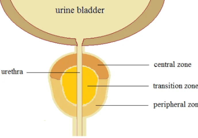
The prostate gland is in the size of a walnut. It starts to develop after puberty, when the testosterone levels rises, and reaches a size of 20 cm2 in a normal adult. From the midlife and forward the prostate gland grows in size, up to double its original size. This can cause pressure on the urethra leading to symptoms that easily can be mistaken for prostate cancer even though this is quite normal. The gland is positioned right below the urine bladder enclosing the upper part of the urethra, Figure 1. The prostate gland consists of two lobes,
one right and one left. The glandular tissue is composed of three zones; peripheral, transition and central zone. Most prostate cancer has its origin in the peripheral zone, about 70 %. [3]
FIGURE 1. The three zones of the prostate.
1.2
D
IFFUSION AND PROSTATE CANCERMonitoring the response of radiotherapy is important for the estimation of the risk for recurrence and to be able to estimate the outcome of treatment. To be able to assess the response from the treatment and to make a prognosis after the treatment, a marker is needed. Today, determination of the prostate size, PSA levels and history taking are methods used as markers.
An increase or persistence of high PSA levels after treatment is strongly connected with a relapse or preserved prostate cancer, however, PSA level has it’s limitation. Even though a decreasing PSA level has been associated with cure and a good response to treatment, 5 to 25 % of the treatment for patients with good response, regarding PSA levels, fails. Also the treatment of patients showing the best response on the PSA testing can fail. PSA level cannot always predict the response of the treatment.[4]
7
Monitoring morphologic changes, like tumor gross size, is used to define response or progression. Even though there is a connection between tumor size and progress this method lacks in interpreting molecular and biological changes in the tumor. The molecular and biological changes can detect early changes, that tumor size are not able to.[4]
Monitoring the size of the prostate during therapy can have other benefits still. If the prostate swells or reduces, during therapy, the target volume will change and this can affect the radiotherapy plan. The placement and size of the target volume will change relatively to the basis for the treatment plan. This can cause under or over dosage of the target volume. When the size can be monitored during treatment, the change in volume can be taken into consideration, either during treatment planning or during treatment.
If the response can be identified during treatment rather than after, the patient can be spared a bad or not efficient treatment. The patient will not be a victim of treatment doing more bad than good, through for example unnecessary toxicity or irradiation of organs at risk. There are many organs at risk close to the prostate, for example urine bladder and rectum, that will despite today´s more advanced treatment techniques, be irradiated. For radiotherapy this result in radiation damages to healthy tissue with poor tumor control. When one are able to assess the response during treatment this opens the way for change or even cancelation of treatment.
It has been shown that diffusion weighted imaging (DWI), especially the apparent diffusion coefficient (ADC), can be used as an early response marker.[4] [5] During radiotherapy the cells undergo apoptosis or necrosis as a response to the irradiation. When the cells die, their membranes will resolve and they will lose their structure. This will lead to a loss of membrane integrity, which will increase the water diffusion in the tissue, in turn leading to an increase of ADC. Also the size and number of cells will decrease after apoptosis and necrosis, increasing the water mobility and the ADC. And hence, a decrease in ADC will reflect a loss of water mobility due to either increasing number of cells, fibrosis or edema.
1.3
A
IMThe aim of the studywas to developaprotocol optimized for measurement ofADC anduse it to determine the precision of ADC measurements. Also to determine the accuracy and reproducibility of volume measurements of the prostate using a T2-weighted sequence.
8
2.
T
HEORY2.1
D
IFFUSIONDiffusion is the random, translational motion of molecules, also called Brownian motion after the botanist Robert Brown who was the first scientist to note this phenomenon in 1827 when looking at pollen grains in fluid. Albert Einstein was the first to in detail describe the Brownian motion. In 1905, Einstein came up with the following relation for diffusion in three-dimensions
< 𝛥𝑟! > =6𝐷𝛥𝑡 ( 1 )
where <𝛥𝑟! > is the average square displacement of a particle during the time interval Δt
and is characterized by the diffusion coefficient D. The relationship statistically describes the average distance the particles move over a time interval. The diffusion motion, which is driven by thermal energy carried by the molecules or particles, is also called self-diffusion. The diffusion coefficient depends on the molecular size, temperature and viscosity of the medium, and in that way incorporate the characteristics of the medium in to the relationship. The diffusion coefficient describes the diffusion characteristics of the medium and isalways the same for a given medium and temperature.
In free water the particle motion is random and equally probable in all directions. The displacement of the molecules obeys a three-dimensional Gaussian distribution.
In vivo, the displacement is not equal in all directions because of interactions between the water molecules and tissue components, like cell membranes, fibers and macromolecules. In biological tissue the diffusion motion of the water molecules is restricted and the diffusion distance is reduced as compared to diffusion in free water. This enables the diffusion to reflect structure and geometric organization of the environment of the water molecules. The diffusion coefficient D is therefore replaced by the apparent diffusion coefficient (ADC), the diffusion coefficient now includes more than the self-diffusion and represents no longer only the diffusion motion.
2.2
D
IFFUSIONMRI
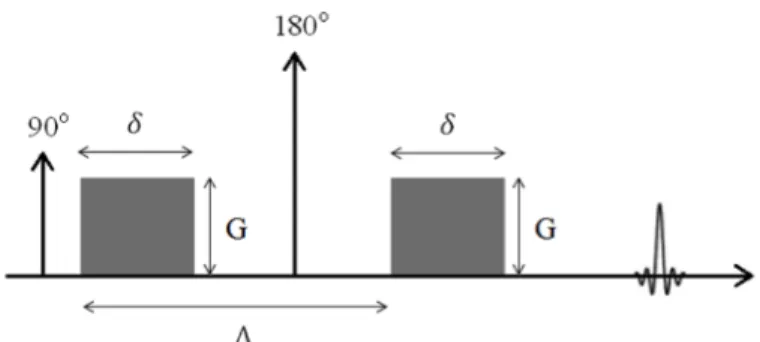
In 1965 Stejskal and Tanner designed a pulse sequence, a pulsed gradient spin echo (PGSE), that was especially suited to detect diffusion motion. [6] The PGSE sequence is still the basis for diffusion sensitive sequences used in MR imaging today. The MR signal is made sensitive to diffusion through two consecutive magnetic field gradient pulses (Figure 2). When a gradient pulse is applied, the protons will experience a diverse magnetic field along the gradient direction. Due to the fact that the magnetic field strength affects the
9
spin’s precession frequency the spins along the gradient direction will precise with different precession frequencies when the gradient is applied. When the gradient pulse is switched of the spins have gained a change in phase angle, 𝜑, due to the gradient pulse, G, that is dependent on the spatial location of the protons, x, along the gradient direction and the duration of the gradient pulse, t’.
𝜑 𝑡 =𝛾 !𝐺(𝑡!)∙𝑥 𝑡! 𝑑𝑡′
! ( 2 )
The gradient pulse labels the spin according to their position along the gradient direction. The second magnetic field gradient pulse is equal in amplitude and duration to the first pulse but opposite in polarity and will therefore refocus stationary spins. If the protons have moved during the time interval between the two gradient pulses the spins will not be fully refocused by the second gradient pulse, which results in a net phase shift. The greater the displacement is, the greater the phase shift will be. For a population of spins the net effect of the remaining phase shift will result in an attenuation of the signal, proportional to the net displacement of the protons. The signal attenuation is described by Equation. 3.
𝑆 𝑏 =𝑆 0 𝑒!!∙!"# ( 3 )
where S(b) is the signal for a certain b-value, S(0) the signal without diffusion weighting
and ADC is the apparent diffusion coefficient. The b-value was first introduced by Le
Bihan in 1986 as a diffusion sensitization factor [7]. The b-value is directional dependent and determined by the direction of the gradient, the gradient amplitude, G, the duration of each diffusion encoding gradient, 𝛿, the time interval between the two gradients, 𝛥, and the gyromagnetic ratio, 𝛾, according to Equation. 4.
𝑏=𝛾!𝐺!𝛿!(𝛥−!
!) ( 4 )
The last term in the equation is described as the diffusion time. By changing these parameters the degree of diffusion weighting can be controlled. A larger b-value will be able to detect smaller displacement of the protons because of the increase in diffusion weighting, however, at the cost of decreased SNR in the overall image. When the b-value increases the duration of the gradients pulses (𝛿) also increases, witch requires a larger TE, which in turn cause a lager T2-relaxation and decreased signal.
10
FIGURE 2. A schematic illustration of a diffusion sensitive pulse sequence.
2.3
A
PPARENT DIFFUSION COEFFICIENTIn biological tissue the diffusion is no longer free due to the interaction with cell membranes, fibers and macromolecules in the tissue. In tissue the signal is not only affected by the effect of the diffusion, but also perfusion and bulk motion, which is to a large extent unavoidable because of the nature of the measurement. Instead of free diffusion a more complex diffusion process occurs which make it more appropriate to use the term apparent diffusion coefficient (ADC), instead of the diffusion coefficient. The purpose of using the ADC parameter is to summarize all physical processes that occur at voxel level. Therefore it can be somewhat difficult to do a direct physical interpretation of this parameter.[8] Even so, the ADC has many useful applications of great value.
The signal decreases with increasing b-value, according to Eq. 3. and by replacing the diffusion coefficient by the apparent diffusion coefficient in Eq 3 the apparent diffusion coefficient can be computed by solving the equation. For two b-values the ADC can be calculated according to the following expression.
𝐴𝐷𝐶 =𝑙𝑛
𝑆(𝑏!) 𝑆(𝑏!)
𝑏!−𝑏! (5)
Where S(b0) and S(b1) is the signal for two different b-values, b0 and b1. For more than two
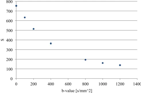
b-values the ADC can be computed by fitting a straight line to the data points, shown in Figure 3.
11
FIGURE 3. The signal in the prostate plotted against the b-value.
When determining ADC the choice of b-values is of great importance.[9]At low b-values the signal attenuation will depend on both diffusion and perfusion. Water and blood in the capillaries will increase the dephasing of the spins and therefore increase the attenuation of the signal. When calculating the ADC the perfusion fraction will lead to an overestimation of the ADC. It is therefore important to choose the b-values in a way that minimizes the effect of the perfusion fraction on the ADC calculation. At higher b-values there is no influence of perfusion, the signal attenuation is only dependent on diffusion. When increasing the b-value the relative noise level also increases due to signal loss. The flattening of the signal curve is due to the approaching of the noise floor. Using a b-value that gives a signal too close to the noise floor can lead to an underestimation of the ADC.
0 100 200 300 400 500 600 700 800 0 200 400 600 800 1000 1200 1400 S b-value [s/mm^2]
12
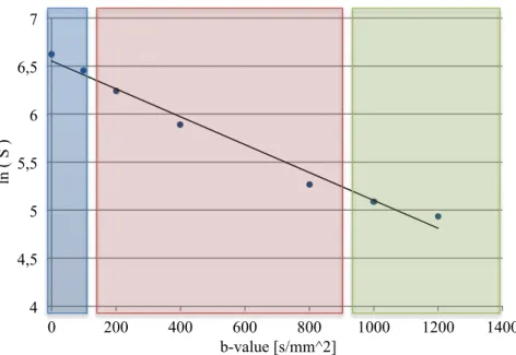
FIGURE 4. The logarithm of the signal plotted against the b-value, with a line fitted to the data points. The blue area indicates the region where the signal is influenced by the perfusion fraction. The red area indicates the region where the slope is mono-exponential and a true estimation of the ADC can be done. The green area indicates the region where the signal is affected by the noise floor.
2.4
P
ITFALLS IN DIFFUSION IMAGING ANDADC
CALCUALTIONSArtifacts are nothing unusual in MRI imaging, especially not in diffusion MRI. Typically DWI artifacts have their origin in the strong gradient pulses used for diffusion weighting of the image. Since the b-value, the strength of the diffusion encoding, is primarily determined by the intensity and duration of the gradient pulse the hardware has to be able to deliver strong and stable gradients.
2.4.1MOTION ARTIFACTS
Diffusion weighted imaging is sensitive to small, microscopic motion of the water molecules and is therefore also sensitive to all motions. Since Echo planar imaging (EPI) made it’s entry in DWI the problem with motions, other than the diffusion motion, has been reduced. By fast acquisition, where the entire image is acquired in one excitation, the images can be collected in about 100 msec, short enough to freeze the motion during acquisition. EPI sequences are nowadays standard for diffusion imaging and have made clinical DWI possible. Parallel imaging can fasten the acquisition time even more, through undersampling of the image. Still there are problems arising from motion for ADC measurements, if the patient moves during the acquisitions of a series of different sensitized images. A given voxel within the image will not have the same location throughout the dataset, causing problems when calculation the ADC.
4 4,5 5 5,5 6 6,5 7 0 200 400 600 800 1000 1200 1400 ln ( S ) b-value [s/mm^2]
13 2.4.2EDDY CURRENTS
When the gradients are switched on and off time-varying magnetic field is created. The time-varying field induces currents, called eddy currents, in the conducting parts of the MRI scanner. The currents in turn create magnetic field gradients which can remain after the main gradients are switched of. The created magnetic gradients add to the imaging gradients in a way that the magnetic field experienced by the spins is affected. When the spins are under influence of an additional magnetic field the image reconstruction will be currupt. The Fourier transformation assumes that data points is placed in a Cartesian grid, however due to effects of eddy currents this is no longer the case since data points will be shifted due to eddy currents. In the reconstructed image this will result in a geometric distortion, both shear, translation and magnification the image. This artifact becomes worse when the diffusion encoding is stronger, hence stronger gradient pulses may lead to greater induced magnetic field.
Since ADC maps are calculated from images obtained with different b-values, where different strength of the gradient pulses is applied, the distortion will differ between the images. Signals from slightly different areas of the images will be used for the calculation. This will result in an inaccurate ADC-map.
One way to solve some of the problems with eddy currents is to use self-shielded gradient coils, which at present are standard in most MRI scanners. The shielding will reduce the effect on the conducting material outside the gradient coils. Still there will be eddy currents in other parts even though coils can be made in a way that reduces the effect. To additionally reduce the effect from eddy currents in the image one can redesign the current sent to the gradient coil in a way that minimizes and compensates for the effect by the eddy currents that are created.
Another way to minimize the effects from eddy currents is to design the pulse sequence in a way that reduces the eddy currents. As a finale possibility to reduce the effects from eddy currents one can take help of post-processing.
2.4.3CROSSTERMS
Not only diffusion pulse gradients are present during the DWI sequence, but also imaging gradient pulses. All of these pulse gradients contribute to the b-value, not only the ones intended. When calculating the ADC this effect will affect the result as the b-value used for the calculation is not the one experienced by the spins.
2.4.4.METAL ARTIFACS
Some prostate cancer patients have gold seeds placed in there prostate during radiotherapy to increase the precision of the positioning of the patient during treatment. When performing ADC measurements on these patients it is important to take into consideration
14
that the gold seeds will cause metal artifacts in the images. Metal artifacts arise from local magnetic field inhomogeneity caused by the metal. The local magnetic field inhomogeneity will change the precession frequency of the protons in that area causing a wrong positioning of the signal in the reconstructed image. This will result in a distortion in the image, with an area with higher signal intensity and one with a lower. In a ADC map this will lead to an miscalculation of the ADC near the gold seed.
15
3.
M
ETHODS AND MATERIALThe study was carried out on both phantoms and healthy volunteers. Phantoms was used in order to make determinations of how accurate the volume can be measured. For determinations of reproducibility of volume and ADC measurements both phantoms and volunteers were used.
All measurements were carried out on a General Electric Discovery MR750w 3 T, placed at the radiotherapy department at Skånes university hospital. A 32 channel cardiac coil was used.
3.1
P
ILOT STUDYTo create the best conditions regarding the number of b-values and number of excitations for determination of ADC in prostate a pilot-study was carried out. To determine the number of b-values to be used for the measurement of the ADC, data from three healthy volunteers was used. Diffusion weighted images was taken with seven different b-values, b = 0, 100, 200, 400, 800, 1000 and 1200 s/mm2. The ADC was calculated using the mean signal in a region of interest (ROI) [8]. The logarithm of the mean signal in the ROI, positioned at the outer parts of the prostate to avoid the urethra, for all seven b-values was plotted against the b-value. The ADC-value was then calculated by fitting a straight line to the data points, using a least square regression. By calculating ADC using both different b-values and different number of b-values, the variation in ADC depending on the choice of b-value could be studied. A Pearson’s correlation coefficient was calculated as a measure of the fitting of the line to the data points. Also the shape of the curve, given by the data points, gave indications on how the b-values best would be chosen to get the most accurate ADC of the prostate. The curve shows in what degree the perfusion fraction and the noise level affects the data points, as described above.
In order to select the higher b-value a measurement and calculation of SNR was done to get an estimation of where the noise level is. The SNR was calculated by acquiring two consecutive images with the same settings using images from one of the volunteers. The images were subtracted one from the other, pixel by pixel, creating a difference image. The difference between the two original images should only be due to noise. The standard deviation of the signal in the difference image is the noise and the SNR was calculated using the following equation.
𝑆𝑁𝑅 = 2∙!! (6)
Where S is the mean signal in a region of interest in one of the original images and 𝜎 is the standard deviation of the signal in the same ROI in the difference image. A change in
16
patient position between the two images will affect the calculated noise, mainly in areas where the change is signal is large. The ROI was therefore placed at a region where the signal is homogeny to reduce potential effects from movements.
3.2
P
HANTOM STUDYTwo different types of phantoms was used, one for the determination of accuracy and reproducibility in volume measurements and one for the measurements of reproducibility of ADC.
3.2.1VOLUME
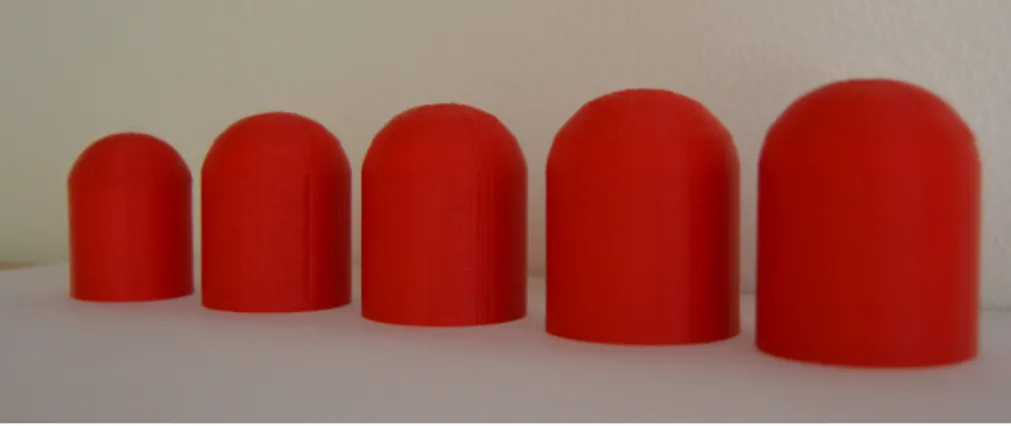
The phantoms were made using a 3D-printer that made it possible to pre-determine the shape and volume of the phantoms. The shape of the phantoms was bullet-like to resemble that of a prostate according to an article by MacMahon et al. [10] The phantoms were made in five different sizes with volumes in the range of a prostate (20 – 50 ml), Figure 5, and in at plastic material. The volume of the phantoms was measured by weighing the phantoms filled with water and thereafter weighing the empty containers and subtracting these two to get the weight of the water filling the phantom. The remaining water in the phantoms after emptying was assumed negligibly small. With the help of the density of water in room temperature (ρH2O=0,998 g/ml) the volume was calculated. This measurement was used as a
reference volume of the phantoms.
The five phantoms was filled with water and placed in a container with water. Images was taken with a T2-weighted propeller sequence identical to the one used clinical for tumor localization of prostate cancer patients treated with radiotherapy. The sequence used the following settings: 20 cm FOV, 0.39×0.39×3 mm voxel size, TR/TE= 4300/110 ms. Imaging of the phantoms volumes was done five consecutive times with a slice thickness of 3 mm.
17
FIGURE 5. The phantoms used for the determination accuracy and precision of volume. They are made using a
3D-printer in five different sizes, with volumes from 20 ml to 50 ml.
The volume measurements were then made in the treatment planning system Eclipse (Varian Medical systems). The contour of the phantom was delineated in each slice, creating a volume representing the phantom. The volume of the phantoms was then calculated by the system.
3.2.2ADC
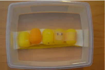
During the measurement for determining the precision of the diffusion coefficient D five plastic containers were used, each one filled with liquids with different diffusion coefficients (Figure 6). Because diffusion is free in free water D is used instead of the ADC. The different diffusion coefficients were produced with the help of sugar. Solutions with different amount of sugar resolved in water will result in different diffusion coefficients. The sugar-water solutions was made in five different weight concentrations, 5, 10 20, 40 and 80 %. The plastic containers were placed in water and measurements were performed with five consecutive repetitions. The results from the pilot-study were used to select the protocol used for this measurement. Two b-values, b=200 smm-2 and b=800 smm-2, with eight excitations each where used for the calculation of ADC. The following settings were used for the acquisition: 0.78×0.78×3 mm voxel size, TR/TE= 4000/90 ms, 20 cm FOV. The ADC was calculated by the built in calculation software in the MR-camera, with a monoexponential fit. This is the way ADCs are calculated clinically and therefore the choice for the calculation in this study.
18
FIGURE 6. The five phantoms filled with sugar-water solutions with different diffusion coefficients.
As described in the theory section the ADC is affected by the unlinearity of the gradients. A cylindrical water phantom was used to determine how the measured ADC varies with position along the tunnel. The phantom was centered at the middle of the tunnel and the ADC was measured with 3 mm intervals superior and inferior of the center without moving the phantom. In this way a profile of the measured ADC along the tunnel was obtained. The following settings were used for the acquisition: 0.74×0.74×3 mm voxel size, TR/TE= 4000/90 ms, 20 cm FOV and b= 0, 100, 200, 400, 800, 1000, 1200 s/mm2.
3.3
V
OLUNTEER STUDYMeasurements were performed on seven volunteers with a mean age of 24.6 years and a median of 24 years and a mean weight of 80 kg. Both measurements for reproducibility of volume and ADC were performed during the same examination. The measurements were repeated two times for each volunteer. Between the two repetitions of the same examination the volunteer got up from the exam table and moved around for a couple of minutes. There was no break and no intake of liquid or emptying of bladder.
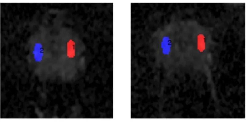
The protocol determined with the help of the pilot study were used for this ADC measurement also. The parameters used was: b= 200 and 800 s/mm2, 20 cm FOV 0.78×0.78×3 mm voxel size, TR/TE= 4000/90 ms. The slices were angulated in the transverse plane to avoid the bladder which can affect the diffusion weighted image because of the high signal arising from the urine in the bladder. The ADC was calculated with the built-in GE soft ware. For each volunteer areas with homogeneous values were matched between the two measurements for placement of ROI, one example is to be seen in Figure 7. The ROIs was placed in the peripheral zone of the prostate. For these
19
measurement values from only six of the seven participating volunteers was used due to deviant and doubtful values of the ADC measurement for one individual. The result from this volunteer was therefore excluded from the study.
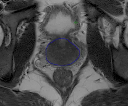
For the volume measurements the same protocol and sequence was used as previously described in the section on method with the following settings: 20 cm FOV, 0.39×0.39×3 mm voxel size, TR/TE= 4300/110 ms. The prostate was delineated, se Figure 8, in the treatment planning system Eclipse (Varian Medical systems), creating a volume representing the prostate. The volume of the prostates was calculated by the system.
FIGURE 7. Example of ROI placements for one of the volunteers. The ROI are placed in a homogeneous area in the peripheral zone.
20
21
4.
R
ESULTS4.1
P
ILOT STUDYThe result from the measurement on three healthy volunteers is presented in Figure 9. The decay of the signal versus b-value curve is changing with increasing b-value. The three volunteers follow the same pattern regarding this decay. In Figure 9 a more rapidly decaying part for b = 0 s/mm2 can be seen, which is due to perfusion. Also a flattening of
the curve can be seen for higher b-values (> 800 s/mm2), because of the signal is beginning to approach the noise level.
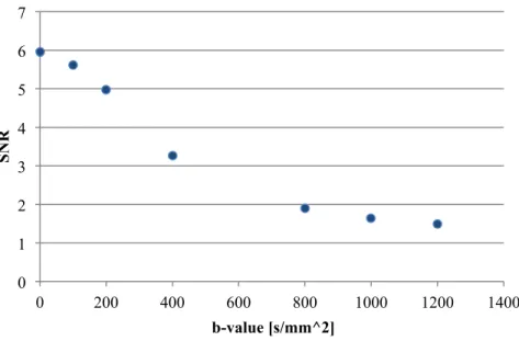
To avoid effects from perfusion on the ADC a b-value higher than 0 s/mm2 must be chosen and therefore the lower b-value was set to 200 s/mm2. At b-values close to 0 s/mm2 the signal is affected by the perfusion fraction but it is not clear at which b-value the signal becomes free from this effect. To avoid choosing a b-value where the signal is based not only on diffusion the lower b-value was set to 200 s/mm2, at 100 s/mm2 the effect on the signal from the perfusion fraction could not be excluded. Based on Figure 10 and calculated Pearson’s correlation coefficients, for different combinations of b-values, it was concluded
that b = 1200 s/mm2 is affected by the noise floor and should therefore not be chosen for the calculation of ADC. The largest b-value was instead set to 800 s/mm2. There were no difference in how good the fitting of the line was for b-values of 200 s/mm2 and 800 s/mm2 or 200 s/mm2 and 1000 s/mm2. The choice was based on calculations of SNR, presented in
Figure 11.
The number of b-values was chosen to two b-values. This result was also concluded from the presented measurements in Figure 9. A third b-value, in the middle, between the highest and lowest b-values, would not contribute to the slope of the line fitted to the data point, hence the ADC, therefore the number of b-values was set to two.
22
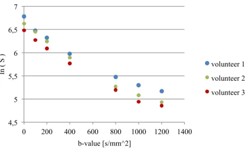
FIGURE 9. Signal versus b-value for three volunteers. The data points follow the same pattern regarding the decay of the signal for increasing b-value.
FIGURE 10. The logarithm of the signal potted against the b-value for seven different b-values, using data from one of the volunteers. The line is fitted to all seven points. This gives a picture of how well the data
points follows a straight line. 4,5 5 5,5 6 6,5 7 0 200 400 600 800 1000 1200 1400 ln ( S ) b-value [s/mm^2] volunteer 1 volunteer 2 volunteer 3 4,5 5 5,5 6 6,5 7 0 200 400 600 800 1000 1200 1400 ln ( S ) b-value [s/mm^2]
23
FIGURE 11. Signal to noise ratio as function of b-value. 0 1 2 3 4 5 6 7 0 200 400 600 800 1000 1200 1400 SNR b-value [s/mm^2]
24
4.2
P
HANTOM STUDY4.2.1VOLUME
An example of images used for the determination the volumes of five phantoms are shown in Figure 12.
FIGURE 12. Example of image used for the determination of accuracy and precision of volume measurements.
The measured weights and calculated reference volumes are presented in Table 1. The volumes measured by MR imaging is presented in
25
Table 2 and Figure 13 for each of the five measurements. To estimate how well the
measured volumes are in consistence with the reference volumes a line was fitted to the data points using a least square fit. The correlation factor is 0.9988 which implies that the consistence between the measured and reference volumes is good. The difference between reference volume and mean volume varies between 1,7% and 6,9%. The variation of the measured volume increases with increasing volume, with a mean deviation for all volume sizes of 2.8 %.
TABLE 1. Measured weights and calculated volumes for the five phantoms.
Phantom Vol 1 Vol 2 Vol 3 Vol 4 Vol 5
Weight water + phantom 24 g 38 g 44 g 55 g 63 g
Weight phantom 4 g 9 g 11 g 13 g 14 g
Weight water 20 g 29 g 33 g 42 g 49 g
26
TABLE 2. Result from the measurements and calculations of volumes of the phantoms. All volumes are given in ml. 1 2 3 4 5 mean stdv % deviation Vol 1 19.2 18.8 18.5 18.4 18.2 18.62 0.39 2.09 Vol 2 27.9 28 29 28.6 27.3 28.16 0.66 2.34 Vol 3 34 34 34.2 33.2 32.4 33.56 0.75 2.25 Vol 4 43.6 44.3 41 44.2 42.2 43.06 1.42 3.31 Vol 5 53.6 53.2 49.2 51.4 49.3 51.34 2.08 4.05
FIGURE 13. The measured volumes plotted against the reference volumes. The error bars shows one standard deviation of the measured values and the line is the identity line. The data points follow a straight line which indicates that the consistence between the reference volume and the measured volume are good
and that the volume reproduction is linear.
4.2.2ADC
The reproducibility of the D was determined with the help of five plastic containers filled with water- sugar solutions with different diffusion coefficient. The measurement was repeated five times and evaluated, the result is presented in Table 3 and Figure 14. As anticipated the D drops with increasing amount of sugar in the solutions, due to the decrease of diffusion coefficient. The standard deviation of the diffusion measurements was calculated for each phantom and a mean percentage deviation was calculated, using the standard deviation of the measurement. The deviation increases with increasing amount of sugar in the solution, and hence the decrease of the diffusion coefficient. The mean percentage deviation was 0.7 %.
15 20 25 30 35 40 45 50 55 60 15 20 25 30 35 40 45 50 55 M eas u re d vol u me [ml ] Reference volume [ml]
27
TABLE 3. The results from the measurements of ADC in five different phantoms with different diffusion coefficients. Sugar-water concentration 1 2 3 4 5 mean stdv % 5 % 1956.7 1942.5 1945.5 1944 1939.4 1945.62 6.6 0.34 10 % 1761.1 1754.5 1754.4 1750.2 1745.6 1753.16 5.8 0.33 20 % 1592.7 1580.9 1583 1572.5 1573 1580.42 8.3 0.53 40 % 1067.1 1051 1060 1060.2 1043.9 1056.44 9.0 0.86 80 % 774.4 777.5 760.9 787.4 757.1 771.46 12.4 1.61
FIGURE 14. Measured and calculated ADC-values for the five different diffusion coefficients.
The result from the measurements on how the unlinearity of the gradients affects the ADC is presented in Figure 15. The measured ADC decreases with increasing distance to the center. If the prostate is 5 cm in the direction parallel to the direction of B0, and well
centered in the middle, the largest deviation from the real ADC, due to the non-linearity of the gradients, would be 2%. The camera will always center over the outlined slices, which in practice means that the deviation of measured ADC values will never differ more than 2%. 0 500 1000 1500 2000 2500 5 10 20 40 80 A D C [mm^ 2/ s] concentration
28
29
4.3
V
OLUNTEER STUDY4.3.1VOLUME
The volume of the prostate was measured in two consecutive examinations for each volunteer and the result is presented in Table 4 and Figure 16. The mean difference between measurement one and two is 1 %. There was an individual difference of prostate volume between volunteers, in the range from 12.6 cm3 to 25.3 cm3. No connection between age and prostate size could be seen.
TABLE 4. Resultsfrom the measurements of the volume of the prostate of seven healthy volunteers.
Volunteer Measurement 1 [ml] Measurement 2 [ml] Difference % 1 18.3 18.95 0.65 1,04 2 20.47 19.46 1.01 0,95 3 20.3 21.7 1.4 1,07 4 25.15 25.25 0.1 1,00 5 19.55 20.24 0.69 1,04 6 18.21 18.08 0.13 0,99 7 12.64 12.68 0.04 1,00
FIGURE 16. Measured volumes for measurement 1 (dark blue) and 2 (light blue) for each volunteer, during two consecutive examinations.
0 5 10 15 20 25 30 1 2 3 4 5 6 7 V ol u me [ml ] volunteer
30 4.3.2ADC
The results from the determination of ADC, measured during two consecutive examinations, for six healthy volunteers are presented in Figure 17. The difference between measurement one and two is in the range from 4 to 18 % with a mean difference of 12%. The differences between volunteers are sometimes greater than the difference between the two measurements for the same volunteer, which is the desired result.
FIGURE 17. The measured ADC, during two consecutive examinations, for six volunteers for measurement one (dark blue) and two (light blue). The error bars indicated one standard deviation of the measured values;
the standard deviation of the values in the ROI used for the measurement.
0 200 400 600 800 1000 1200 1400 1600 1800 1 2 3 4 5 6 A D C [mm^ 2/ s] volunteer
31
5.
D
ISCUSSION5.1
P
ILOT STUDYThe b-values to be used was chosen to b = 200 s/mm2 and 800 s/mm2. There is no other study, in knowledge of, that has used these two b-values when looking at the ADC of prostate from an oncology point of view. In Diffusion- Weighted MR Imaging: Applications in the body [12] a number of calculated ADC in the prostate with different b-values are presented. In contrast to this study many of the studies presented has used a b-value of 0 s/mm2 as the lowest b-value. The number of b-values used is in the range from two to five and the values used are in the range from 0 to 1000 s/mm2.
The choice of b-values and the number of b-values is important for the calculation of ADC. Both the noise floor and the perfusion fraction affect the measured value. To avoid influence of perfusion and overestimation of ADC the lower b-value should be chosen higher than zero.[9] At b=200 s/mm2 one can be fairly sure that there is no perfusion fraction affecting the ADC, because the slope of the signal curve is lower around b=200 s/mm2 than for lower b-values. The SNR drops with increasing b-value as expected. At
b-value of about 800 s/mm2 the SNR flattens out which indicated that the noise floor is reached. Because of the noise level a highest b-value should be set so that the signal is adequately above the noise level.
The number of b-values was chosen based on findings from own measurements and by support from results by Eis and Hoehn-Berlage [11]. Eis and Hoehn-Berlage came to the conclusion that two b-values with high number of acquisitions are better than many b-values with few acquisitions. The question arises from the need for reducing the scan time, which not enables both many b-values and many acquisitions.
5.2
V
OLUME DETERMINATIONThe precision and accuracy of volume measurements was determined by measuring the volume of different sized phantoms and volunteers five respectively two repetitive times. From the standard deviation of the five measurements on phantoms the conclusion, that the volume can be determined with a precision of 3%, was made. The volume measurements of the volunteers were found to have a precision of 1 % between the two measurements. Due to the lake of measurements for calculations for volunteers no comparison between the phantom and volunteer calculations of precision can be made directly. The precision of the phantom study is expected to be better than for the volunteer study. The volunteers moved between the two measurements resulting in different placements of the prostate. In the phantom case there were no movements or change of placement between the measurements. Therefore the phantom study only includes changes due to the imaging of
32
the MRI camera and the delineation and volume calculation. The volunteer study also includes changes of the placement of the prostate, not only in the cameras reference system but also in the volunteer. Therefore the precision in the volunteer study is expected to be larger than in the phantom study.
The precision decreases with increasing volume, this can be due to fact that the same change in delineation of the prostate results in a larger change in the total volume of a larger prostate volume than for a smaller volume. Figure 18 shows how the volumes of the prostate changes with increasing change of radius. A change in diameter of the prostate from 2.8 cm to 3.2 cm would result in a change in volume from 18,5 ml to 21,2 ml (15%). This means that a relatively small wrong delineation in each slice of the prostate can result in a large change in calculated volume.
FIGURE 18. The change in volume due to change in radius of the prostate with a slice thickness of 3 mm.
The accuracy of the measurements was determined by comparing the measured volumes with the reference volume. This comparison came to the conclusion that the consistence is good, with a Person correlation coefficient of 0.998, and a mean accuracy of 3.7%. A study by Gunnlaugsson et al.[14] investigates the swelling of the prostate during radiotherapy comes to the conclusion that the prostate swells at mean 14 % during radiotherapy. In comparison with this result the result from the phantom study can conclude that the prostate can be determined with an accuracy good enough to detect a change in volume of the prostate. This conclusion also includes volunteer and patient measurements. Due to the fact that the absolute volume of the volunteer’s prostate can´t be found no comparable measurement can be done for volunteers. Therefore the result from the measurements of accuracy for phantoms is also assumed applicable for patient measurements. The accuracy
0 50 100 150 200 250 0 10 20 30 40 50 60 % c h an ge in vol u me of th e p ros tate
33
is affected by the delineation in the same way as the precision and is the main reason for a deviation between the real volume and the measured. From this result the conclusion that measurement using a T2-weighted propeller sequence can be used for determining the volume of the prostate.
The result from the determination of the volume is mainly dependent of how the prostate is delineated. Sometimes it can be hard to define where the prostate begins and ends; which slices is containing the upper and lower parts of the prostate. If a slice is included in the prostate volume or not can affect the volume more than a change in delineation in one slice. A smaller slice thickness can make the delineation of the prostate easier by making the boundaries of were the prostate begins and ends clearer. One slice will not affect the total volume to the same degree when the slices are made smaller and therefore is the inclusion or not of a slice as crucial. It is important that the prostate is delineated with the same criteria’s or by the same person. To increase the precision of the measurements clear criteria’s should be set up, so that the delineation is equally done both times. Otherwise no comparison between the two measurements can be done and no conclusions, regarding changes in prostate volume, can be drawn. In this study the delineation was done by the same person and at one moment in time. Therefore, this study can be considered fulfill the above described conditions for making comparisons.
5.3
ADC
DETERMINATIONSDetermination of precision of ADC measurements of the prostate was done on phantoms and volunteers. Measurements on phantoms had a precision of 0.7 %. This gives an indication on how well the system can, repeated times, determine the ADC. The standard deviation of the measured ADC increases with decreasing ADC, this is because the signal in the DWIs decreases with increasing diffusion, hence increasing the noise in the images. The measurements on volunteers gave a much larger deviation between the two measurements. This is mainly due to the difficulty of defining two similar areas in the prostate in the two datasets to compare. The measurement on volunteers gives an estimate, in addition to the system’s ability, of how great impact the in vivo situation has on the ADC comparison.
The differences between measurement one and two for the volunteers has a mean difference of 12 %. This is to be compared with results from studies investigating the change in ADC during radiotherapy, which is the intended use for the result from this study. Park et al [4] found a mean difference in ADC between measurement before starting radiotherapy and three weeks in to therapy of 7.3 %, from mean ADC of 1650 mm2/sbefore to mean ADC of 1530 mm2/s after therapy in the prostate. This difference would not have been found from the results of measurements on volunteers.
34
To be able to make a comparison and to evaluate if the ADC has changed in the prostate, during the time interval between measurements, the ROI has to be placed at the same region in both measurements. Otherwise, nothing can be said about a possible change in ADC. To get the most optimal positioning of the ROI the placement has to be done with good knowledge of the prostate anatomy, allowing accurate placement of the ROI. Also directions of how the placement should be done are of importance and it is desirable that the same person makes the ROI definition in both data sets. This study is lacking in one aspect of the above described points, the result could be even better if a person with greater knowledge of the anatomy of the prostate would do the ROI definition. The definition in this study was sometimes difficult and another, a more skilled person, might have done it with greater accuracy. However, there was not this possibility when the study was performed, therefore definition have been made to the best of ability.
Consideration must also be given to eventual hemorrhage and gold seeds. These will give incorrect ADC values and ROIs must not be placed at these region. In the ADC map it can be hard identify a gold seed and therefore it can be necessary to also take a look at the T2-weighted image to make sure of a good placement of the ROI.
35
6.
C
ONCLUTIONSA protocol optimized for ADC measurements in the prostate was found. It consist of two b-values, b = 200 s/mm2 and b = 800 s/mm2. The ADC can be determined, with this protocol, with a precision of 0.7 % for phantom measurements and 12 % for volunteer measurements. The placement of the regions for ADC measurements is important for the accuracy of a comparison. The regions to be compared must be in the same area of the prostate and gold seeds and hemorrhages must be taken in to consideration. Volume measurements can be made with a precision of 3 %. The delineation of prostate in each slice is of importance but also the definition of the upper and lower part of the prostate. Clear criteria’s has to be set up for the delineation and it is preferred that the same person makes the delineation both times, if a comparison of prostate volume is to be made.
36
7.
A
CKNOWLEDGMENTSFirst of all I would like to thank all of volunteers participating in the study, without whom this thesis would not be possible, and for their time and effort.
A would like to thank my supervisors for their knowledge, support and guidance during this project.
Special thanks are addressed to the staff on the MRI camera, Görel and Senada, for their time, help and for always being encouraging.
37
8.
R
EFERENCES
1. Ringborg, U., R. Henriksson, and T. Dalianis, Onkologi. Vol. 2 uppl. 2008, Stockholm: Liber.
2. Cancerfonden. Prostatacancer. 2014 [cited 2014 22 may]; Available from: http://www.cancerfonden.se/sv/cancer/Cancersjukdomar/Prostatacancer/.
3. Deagupta, P. and R.S. Kirby, ABC of Prostate Cancer. 2012: Blackwell Publishing.
4. Park, S.Y., et al., Early changes in apparent diffusion coefficient from diffusion-‐weighted MR imaging during radiotherapy for prostate cancer. Int J Radiat Oncol Biol Phys, 2012. 83(2): p. 749-‐55.
5. Foltz, W.D., et al., Changes in apparent diffusion coefficient and T2 relaxation during radiotherapy for prostate cancer. J Magn Reson Imaging, 2013. 37(4): p. 909-‐16.
6. Stejskal, E.O. and J.E. Tanner, Spin Diffusion Measurements: Spin Echoes in the Presence of a Time-‐Dependent Field Gradient. The Journal of Chemical Physics, 1965. 42(1): p. 288.
7. Le Bihan, D., et al., MR Imaging of Intravoxel Incoherent Motions: Application to Diffusion and Perfusion in Neurologic Disorders. Radiology, 1986(161): p. 401-‐407. 8. Le Bihan, D., Apparent diffusion coefficient and beyond: what diffusion MR imaging can
tell us about tissue structure. Radiology, 2013. 268(2): p. 318-‐22.
9. Thormer, G., et al., Diagnostic value of ADC in patients with prostate cancer: influence of the choice of b values. Eur Radiol, 2012. 22(8): p. 1820-‐8.
10. MacMahon, P.J., et al., Modified prostate volume algorithm improves transrectal US volume estimation in men presenting for prostate brachytherapy. Radiology, 2009. 250(1): p. 273-‐80.
11. Eis, M. and M. Hoehn-‐Berlage, Correction of gradient crosstalk and optimization of measurement parameters in diffusion mri imaging. Journal of Magnetic Resonance, 1995. 107: p. 222-‐234.
12. Beart, A.L., et al., Diffusion-‐Weighted MR Imaging Applications in the Body. 2010, Berlin Heidelberg: Springer-‐Verlag.
13. Regionalt cancercentrum syd. Vårdprogram för prostatacancer. 2013, Lund.
14. Gunnlaugsson, A., et al., Change in prostate volume during extreme hypo-‐fractionation analysed with MRI. Radiat Oncol, 2014. 9(22).