Modeling of Optimized Neuro-Fuzzy Logic Based Active Vibration Control Method for Automotive Suspension

(1)

Grand Valley State University

ScholarWorks@GVSU

Masters Theses Graduate Research and Creative Practice

1-2019

Modeling of Optimized Neuro-Fuzzy Logic Based

Active Vibration Control Method for Automotive

Suspension

Mohammad Adom Safihulla

Grand Valley State University

Follow this and additional works at:https://scholarworks.gvsu.edu/theses Part of theAutomotive Engineering Commons

This Thesis is brought to you for free and open access by the Graduate Research and Creative Practice at ScholarWorks@GVSU. It has been accepted for inclusion in Masters Theses by an authorized administrator of ScholarWorks@GVSU. For more information, please contact

[email protected].

Recommended Citation

Safihulla, Mohammad Adom, "Modeling of Optimized Neuro-Fuzzy Logic Based Active Vibration Control Method for Automotive Suspension" (2019).Masters Theses. 921.

(2)

Modeling of Optimized Neuro-Fuzzy Logic Based Active Vibration Control Method for Automotive Suspension

Mohammad Adom Safiullah

A Thesis Submitted to the Graduate Faculty of GRAND VALLEY STATE UNIVERSITY

In

Partial Fulfillment of the Requirements For the Degree of

Master of Science in Engineering

School of Engineering

(3)

3

Dedication

(4)

4

Acknowledgements

I would like to thank my thesis supervisor Dr. Nicholas Baine first. He guided me when I felt lost and whenever I needed help he was there to support. I am especially grateful for his guidance on the literature writing, without his supervison this thesis would not be possible. I would also like to thank Dr. Shabbir Choudhuri for his help with this thesis. His expertise and suggestion was immensely helpful and made this thesis a better work. I also owe gratitude to Dr. Ryan Krauss for his encouragement during this work.

Finally I must express my gratitude to my parents and younger siblings for supporting me continuously from the other side of the world. I am also grateful to all my friends and wellwishers, this accomplishment would not have been possible without their encouragement.

(5)

5

Abstract

In this thesis, an active vibration control system was developed. The control system was developed and tested using a quarter car model of an adaptive suspension system. For active vibration control, an actuator was implemented in addition to the commonly used passive spring damper system. Due to nature of unpredictability of force required two different fuzzy inference system (FIS) were developed for the actuator. First a sequential fuzzy set was built, that resulted lower vertical displacement compared to basic damper spring model, but system had limited effect with disturbances of higher magnitude and continuous vibrations (rough road). To improve the performance of the sequential fuzzy set, the main fuzzy set was improved using an adaptive neuro fuzzy inference system (ANFIS). This model increased the performance substantially, especially for rough road and high magnitude disturbance scenarios. Finally, the suspension’s spring constant and damping co-efficient was optimized using a genetic algorithm to further improve the vibration control properties to achieve a balance of both ride stability and comfort. The final result is improved performance of the suspension system.

(6)

6

List of Illustrations

Number Description Page

Figure 1 Quarter Car Model 11

Figure 2 Triangular membership function of fuzzy set 18 Figure 3 (a) ANFIS Fuzzy reasoning (b) structure (c) Gaussian membership

function

21

Figure 4 Scattered Crossover 29

Figure 5 Process Flow for Suspension Model 30

Figure 6 (a) Road Bumps 34

Figure 6 (b) Pothole 34

Figure 7 (a) Rough Road 34

Figure 7 (b) Combined Road Disturbance 34

Figure 8 Steps in development of system 35

Figure 9 (a) Block diagram of Fuzzy Inference System 36 Figure 9 (b) Block diagram for sequential Fuzzy decision 36 Figure 10 Surface Plot for (a) Larger Fuzzy Set, (b) Smaller Fuzzy Set 39 Figure 11 (a) Membership function for displacement before Neural Training 41 Figure 11 (b) Membership function for displacement after Neural Training 41 Figure 12 (a) Training error using Hybrid Neural Learning method 42 Figure 12 (b) Training error using Back propagation Hybrid Neural Learning

method

42

Figure 13 Membership function for Fuzzy and Neuro Fuzzy System. a) Input displacement (Fuzzy)

b) Input velocity (Fuzzy) c) Output force (Fuzzy)

d) Input displacement (Neuro Fuzzy) e) Input velocity (Neuro Fuzzy)

43

Figure 14 (a) Surface Picture of regular FIS (b) Surface of FIS trained with Neural Learning

(9)

9

Figure 15 Number of Peaks, p 45

Figure 16 Disturbance vs displacement of quarter car mass with FIS controlled actuator

48

Figure 17 Displacement of QCM mass with FIS controlled actuator and without any actuator

49

Figure 18 Force under FIS system 50

Figure 19 Comparison of Displacement with ANFIS and with FIS 51

Figure 20 Comparison of Force applied with ANFIS and with FIS 51

Figure 21 Convergence of Optimization 52

Figure 22 Stopping criteria for GA optimization 52

Figure 23 Fitness value from 100 random run 54

Figure 24 Displacement comparison between GA optimized ANFIS and ANFIS

54

Figure 25 Force comparison between GA ANFIS and ANFIS 55 Figure 26 Displacement comparison between GA ANFIS and ANFIS time 5 to

12 sec

56

Figure 27 Force comparison between GA optimized ANFIS and FIS 56

Figure 28 Fuzzy Input and outputs 60

Figure 29 Surface Plot for (a) Combined output area, (b) Combined output with COG (red mark)

(10)

10

List of Table

Table 1 Quarter car properties 32

Table 2 Larger Range Fuzzy set parameters 37

Table 3 Larger fuzzy membership table 38

Table 4 Smaller Range Fuzzy set parameters 38

Table 5 Smaller fuzzy membership table 38

Table 6 Training data for Neuro-Fuzzy System. 40

Table 7 Result from different optimization run 53

Table 8 Fitness data from 100 randomly generated damping co-efficient and spring constant

62

(11)

11

1. Introduction

Vibration isolation and control of a suspension is a popular topic of study in the automotive industry. In this research, a quarter-car model is studied along with active vibration control. An active element (actuator) is used to apply force on the car body to continuously control vibration, and a fuzzy logic controller is used to determine how much force is to be applied.

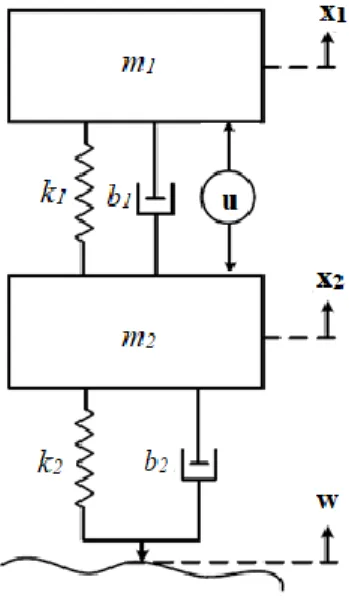
Quarter Car Model (QCM) is used to study the vibration on a car. QCM simplifies the study but provides a representative result for the vibration and corresponding impact on the car. For this general vibration study, the QCM consist of two springs and two dampeners, one for suspension and another representing the tire of the car [1]. For this active suspension model, an actuator was added to mitigate the impact of vibrations in the road disturbance on the displacement of the car between the mass of the car and the wheel. This QCM model is depicted in Figure 1 with the actuator.

(12)

12

Here, m1 is mass of quarter car, k1 is spring constant of suspension, b1 is dampening

coefficient of suspension, x1is vertical displacement of car, m2 is mass of wheel, k2 is spring

constant of tire, b2 is dampening coefficient of tire, x2 is vertical displacement of wheel, w is road

disturbance and u is the actuator force applied.

The force applied by the actuator is calculated using a Fuzzy Inference System (FIS). FIS is a human experience-based approach to make a computation that is not well defined mathematically [2]. However, the rule base for a traditional fuzzy logic controller is limited by the scope and capabilities of human experience and abilities. To work around this limitation, neural learning can be a useful method to improve upon the FIS model, with the system being trained to generate its own rule base based on a given set of training data. The combination of the two concepts is referred to as an Adaptive Neuro Fuzzy Inference System (ANFIS), which has a fuzzy set where the rule base is result of neural training based on data provided from human experience.

While neural learning is known to be inspired by the functioning of human brain, Genetic Algorithms (GA) are based on natural selection. The third method used to improve performance is GA optimization, which is based on survival of fittest principle. A genetic algorithm will be used to optimize the system being controlled. This works by creating multiple versions of the system and comparing their performance. The best designs survive and are mixed to create the next generation of designs. In each generation, GA optimization generates a new population keeping only the best designs to be used to create subsequent populations. Eventually, the algorithm will converge on an optimized solution with a better performance than any of the initial designs in the first population.

(13)

13

1.1. Objective

In this work, a second-order differential equation of forced damped vibration for a quarter car suspension model is used. The objectives of this research work are:

 Development of a state-space model for forced damped vibration  Modelling of quarter car based on previous studies

 Developing a FIS model for active vibration control of a suspension  Improving fuzzy rule base with ANFIS training

 Optimizing suspension system parameters using a GA to further improve performance

1.2. Scope

This work models an active suspension system using a quarter car model, where the active force calculation system was developed using FIS and ANFIS methodology and the performance was compared. For FIS, the Mamdani inference system was used. For ANFIS the Takagi-Sugeno method and hybrid method were used for training. Finally, a genetic algorithm was used for optimization of the actual system model design. The system was limited to two masses and parameters were constrained as there are realistic limitations.

(14)

14

2. Background and Literature Review

In various industries, noise and vibration control is an important concern. In the conventional spring damper system, springs store energy and dampeners dissipate the energy to reduce the effect of vibration. In a passive suspension system, there is no control of the spring and dampener; therefore, the vibration cannot be isolated and used to provide feedback. For the modern automobile vibration, researchers have improved upon the passive suspension through the development of active and semi-active vibration control studies. In semi-active suspension systems, vibration control is improved by changing the physical properties of suspension at certain stages. Alternatively, active suspension systems work by continuously monitoring and injecting the proper amount of force through an actuator attached with a conventional suspension.

The active control of vibration is a popular research topic, with much work being done using both theoretical and experimental studies [3]. The comfort and maneuverability of a vehicle depends heavily on the response of the suspension and its ability to reject disturbances (i.e. vibration control). Semi-active suspension performs adequately in most scenarios, but with the growing possibility of the driverless car in the near future and increasing demand of smoother vibration control, active vibration control is being explored as a better solution according to Pinhas Barak [4]. His work predicted that active vibration control will be able meet the demand of the future, as new developments make it more practical to implement. Dean Karnopp in his study used [5] the skyhook damper model for the active suspension system with vibration control. This study also compares the active and semi-active suspension. The basic Skyhook damper system only used damping to control the vibration, but it has its limitation in flexibility and operation in the robust system. Scott Ikenaga et al. developed an active suspension control for a full car model using a control system that combines filtered feedback and input decoupling transformation [6]. They used

(15)

15

skyhook damping and mitigated the vibration by actively controlling the damping coefficient of a semi-active damper. For the nonlinear system, the skyhook damper has few limitations. For better flexibility and response Krtolica and Hrovat solved a fourth-order linear quadratic differential equation for a half-car model in order to find the optimal solution to vibration control [7].

For the nonlinear system, Ozgur Demir et al. used fuzzy logic combined with a PID controller for a suspension design of a half-car model [8]. Fuzzy logic improves the control of the nonlinear system, and in the robust nonlinear system, the fuzzy logic system can react fast and has great performance [9]. Qu Wenzhonga et al. have shown the advantage of fuzzy logic over filtered-X LMS algorithm [10]. They proved that use of fuzzy logic can be advantageous over an algorithm like filtered-X LMS, which is simple to use and requires low computational load but is more suitable for linear control problems. Shiuh-Jer et al. [11] have designed an adaptive fuzzy controller using the sliding mode controller, where a smaller rule base is required, but they implemented online learning to compensate the system’s time-varying and nonlinear behavior. Jinpeng Li et al. [12] elaborated on the coupling of fuzzy logic and sliding mode controller where they designed an adaptive fuzzy system for a semi-active suspension system.

Implementation of online and different machine learning is also becoming common in vibration studies. M Soleymani et al. [13] used online learning to make the suspension system react with not only road conditions but also traffic conditions. Various machine learning and genetic algorithm are also being used to design robust fuzzy logic control systems. Wei-Yen Wang et al. [14] used neuro-fuzzy logic, and Tomonori Hashiyama et al. [15] used the genetic algorithm with fuzzy logic to control an active or semi-active suspension.

Neuro-fuzzy and genetic fuzzy algorithm-based suspension is more robust and efficient compared to the traditional fuzzy algorithms, but they are more computation heavy to train. In

(16)

16

either case, the fuzzy logic itself is computationally light and can be implemented on low-end suspension with little cost increase for application. In a complex non-linear system, the rule base often gets very convoluted. In this study, a sequential fuzzy set approach is explored instead of one monolithic fuzzy set; this provided scope to focus rules to specific conditions and allowed for an easy to comprehend and editable rule-base for the fuzzy set. However, after development, the sequential fuzzy set could be changed to a monolithic fuzzy set with no significant performance change.

2.1. Fuzzy Inference System (FIS)

In this work, a quarter car model was used as the plant to study fuzzy logic based active vibration control. Mamdani model for the fuzzy set was selected as it provides a simpler rule interface. Rules in a Mamdani set can be developed over human experience. This is in comparison to the mathematical rule base in Takagi-Sugeno among other fuzzy approaches. For membership functions, simplicity and effectiveness of isosceles triangles were used by Manu Sharma et al. [16]. They have studied the effect of the right-angled and isosceles triangle on Mamdani type Fuzzy control system. Grzegorz Filo [17] showed ways to use MATLAB/Simulink’s fuzzy logic developer to model fuzzy control effectively [17]. For work in this thesis, triangular membership functions were chosen for the fuzzy sets and implemented in MATLAB

The FIS process can be broken into three main steps. Fuzzification, rule generation, and defuzzification.

2.1.1. Fuzzification

Fuzzification is at the beginning of the FIS. It is where the system takes a crisp value (real scaler number) and converts it into a fuzzy linguistic value. For any certain crisp value, a

(17)

17

corresponding fuzzy value can be created as part of different classes of fuzzy membership functions. These membership functions are what define how the crisp value is converted.

There have been a variety of proposed fuzzy membership functions proposed, but according to Zadeh [2] they can all be classified as one of two types: one type consisting of straight lines and one made of curves. Curved membership functions are computationally heavier but perform well for non-linear systems; however, the advantages are limited. Consequently, straight or linear membership functions are more widely used, as they are easy to develop and computationally light.

Triangular fuzzy membership functions are the simplest to develop. Witold Pedrycz [18] and Manu Sharma et al. [16] showed that satisfactory results can often be achieved using triangular membership functions. So initially, this study used triangular membership functions to develop fuzzy set for both a larger and smaller FIS.

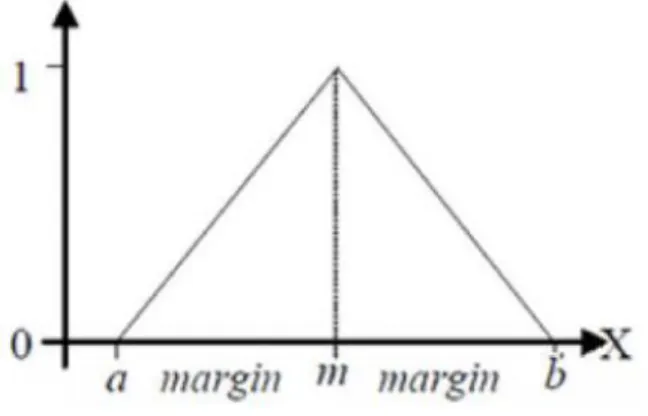
As seen in Figure 2, triangular membership functions are defined by two limits and a mode. The lower limit is shown as a, the upper limit is b, and the peak of the triangular membership function is at the mode m. The function is defined over the range a < m < b with a maximum value of one.

(18)

18

Figure 2: Triangular membership function of fuzzy set

2.1.2. Fuzzy Rule Base

The rule base for a fuzzy system is designed with the experience and reasoning of humans. When the relationship between input and output can be defined through basic logic, one can express these relationships as rules in the form of if-then statements (e.g. “if the input is positive and large, then the output is negative and large”). “Positive and large” from the example would be defined by a membership function. The term is not represented by a precise value, but rather it is defined as a range over which an input can be characterized as having partial membership (0-1[100%]) to the term.

Other examples of rules are

 If input 1 is P and input 2 is Z, then output is N

 If input 1 is N and input 2 is N, then output is PL

 If input 1 is Z and input 2 is Z, then output is Z

(19)

19

2.1.3. Defuzzification

Defuzzification is the process by which a crisp output value is derived from fuzzy parameters. Mitsuishi & Shidama [19] described defuzzification process as converting membership degrees of fuzzy sets to a specific value. There are quite few defuzzification methods available. The most popular methods are the center of gravity method, the center of area method, and the center-average method. For initial fuzzy sets, center of gravity method is used for defuzzification. A crisp value is extracted based on the center of gravity of fuzzy set. Using the center of gravity method, the crisp value 𝑧∗ is expressed as:

𝑧∗₌ ∫ µ(𝑧). 𝑧𝑑𝑧 ∫ µ(𝑧). 𝑑𝑧

where 𝑧∗_{is a fuzzy variable, µ(𝑧) is the area of membership value and z is centroid of the area.} The resultant action is divided or distributed into multiple sub areas from different membership function. The resultant area and center of gravity is calculated to find the final

Effectively the equation becomes

𝐶𝑟𝑖𝑠𝑝 𝑣𝑎𝑙𝑢𝑒 = 𝛴𝑎𝑟𝑒𝑎 ∗ 𝑐𝑒𝑛𝑡𝑟𝑜𝑖𝑑 𝑜𝑓 𝑎𝑟𝑒𝑎 𝛴𝑎𝑟𝑒𝑎

(20)

20

2.2. Adaptive Neuro Fuzzy Inference System (ANFIS)

A fuzzy logic controller is useful for designing an intelligent and robust controller and works well on non-linear processes; however, the design process of fuzzy logic controllers is not formalized [20]. Neural networks can be used to tune fuzzy logic set and improve the rule base of a fuzzy controller. This is done with the use of training data [2]. ANFIS utilizes Takagi-Sugeno fuzzy inference system, which is generated and then improved by neural network training. [21] [22]

The ANFIS is one of many methods known as neuro-fuzzy. Adaptive neuro-fuzzy inference system (ANFIS), was first proposed by Jang (1993) [22] and is based on the first-order Takagi-Sugeno fuzzy model. Generally, ANFIS uses either back-propagation or a combination of least square estimation and back-propagation for membership function parameter estimation (Jang and Sun, 1997 [24]). The most important goal of combining fuzzy systems with neural learning capabilities is to implement the robust learning ability of neural networks, which is not part of a regular FIS system. This combination of neural network and FIS allows for the system to learn, improving the performance of the controller. In ANFIS, a Takagi–Sugeno type fuzzy inference system is used to model the system. In Takagi-Sugeno inference systems, the output of each rule is either a linear combination of input variables plus a constant term or only a constant term. The output then consists of a weighted average of every rule’s output. This integrated approach, makes ANFIS a universal estimator [25].

Figure 3 shows an ANFIS architecture that was proposed by (Ahmed et al. [26]) that has two inputs x and y and one output f. The rule base contains two Takagi–Sugeno if-then rules as follows:

(21)

21

(22)

22

Rule 1: If x is A1and y is B1, then 𝑓1 = 𝑝1𝑥 + 𝑞1𝑦 + 𝑟1; Rule 2: If x is A2 and y is B2, then 𝑓2 = 𝑝₂𝑥 + 𝑞₂𝑦 + 𝑟₂ [22]. Figure 3(a) shows the representative fuzzy sets, and Figure 3(b) depicts the training methodology used to change membership functions. Layer 1 is the node function. Layer 2 calculates the product of the node function signals. Layer 3 normalizes the results of Layer 2 by calculating the ratio of each activated rule strength to all activated rules strengths. In layer 4, the output for each node function is calculated, and layer 5 calculates the overall output.

2.2.1. Hybrid Training Method

Hybrid method of training an ANFIS is a combination of least square estimation and back-propagation for membership function parameter estimation [24]. An adaptive network is a multilayer feedforward network where every node performs a particular function referred to as a node function. The node function can vary on each individual node. If a given adaptive network consists of L layers and kth layer has #(k) nodes. The node in ith position and kth layer can be denoted by (k,i) and node output can be expressed as 𝑂_𝑖𝑘 . A node output is a summation of incoming signals and can be expressed as

𝑂_𝑖𝑘 = 𝑂_𝑖𝑘(𝑂_𝑖𝑘−1, … 𝑂_#(𝑘−1)𝑘−1 , 𝑎, 𝑏, 𝑐, … ) (1) where a,b,c… are parameters related to each node.

If a training data has P entries, the error measure Ep, for the pth (1 ≤ 𝑝 ≤ 𝑃) entry can be

presented as a sum of squared errors, yielding

𝐸𝑝 = ∑ (𝑇𝑚,𝑝− 𝑂𝑚,𝑝𝐿 ) 2 #(𝐿)

𝑚=1

(2)

where 𝑇_𝑚,𝑝 is the mth component of pth target output vector, and 𝑂_𝑚,𝑝𝐿 is the actual output of mth component. To use the gradient decent method for neural network learning, the error

(23)

23 𝜕𝐸𝑝

𝜕𝑂_𝑖,𝑝𝐿 = −2(𝑇𝑖,𝑝− 𝑂𝑖,𝑝

𝐿 ₎ (3)

The error rate at the internal node (k,i) can be similarly derived using chain rule:

𝜕𝐸𝑝 𝜕𝑂_𝑖,𝑝𝑘 = ∑ 𝜕𝐸𝑝 𝜕𝑂_𝑚,𝑝𝑘+1 𝜕𝑂𝑚,𝑝𝑘+1 𝜕𝑂_𝑖,𝑝𝑘 #(𝑘+1) 𝑚=1 (4)

Assuming 𝛼 is a parameter of the network, equation (4) can be expressed as

𝜕𝐸𝑝 𝜕𝛼 = ∑ 𝜕𝐸𝑝 𝜕𝑂∗ 𝜕𝑂∗ 𝜕𝛼 0∗_𝜖𝑆 (5)

where S is the set of nodes whose output is dependent on 𝛼. Taking the derivative of E with respect to 𝛼 yields 𝜕𝐸 𝜕𝛼 = ∑ 𝜕𝐸𝑝 𝜕𝛼 𝑃 𝑝=1 (6)

Now Δ𝛼 can be expressed as

𝛥𝛼 = −𝜂𝜕𝐸 𝜕𝛼

(7) where η is the learning rate and can be expressed as

η = 𝑘 √∑(𝛿𝐸

𝛿α) 2

(8) with k as the step size (length of parameter space gradient transition). The k parameter can be used to affect the speed of convergence.

There is two type of hybrid learning: off-line and on-line. In online learning, parameters are updated after each epoch. In this research, off-line batch learning was implemented. This method combines a gradient method and least square estimate (LSE) to identify system parameters.

(24)

24 Assuming the adaptive network has a single output

Output = F (𝐼⃗, S)

where I is input variables set (for this problem only 2 variable), S is parameter set, and F is function implemented by ANFIS. If there exists a composite function, then H ○ F is linear for all values of S, then these values of S can be identified by LSE. If S is decomposed such way that S1 ⊕ S2 = S,

then

H(output) = H ○ F (𝐼⃗, S) (9)

The training data set contains P data pairs. To successfully train the system, P must be greater than than number of linear parameters M. Assuming H(output) will be linear under the elements of S2,

the equation can be simplified by putting P into (1), yielding

Ax = b , (10)

where x is an unknown vector and S2 is represented by the elements of x. Let |S2| = M, then the

dimensions of A, x, and b will be equal to P × M, M × 1 and P × 1. If P > M, equation (10) does not have an exact solution, instead to minimize the squared error of ||𝐀𝐱 – 𝐛||𝟐_,_x*_{, the least}

squares estimate (LSE) of x, is calculated. The formula used for x*_is

x* = (AT_A)-1_AT_b ₍₁₁₎

where (AT_A)-1_AT_{is the pseudo-inverse of}_A_.

Finally, the results from the gradient method and the least square estimate are used to update the adaptive network parameters. Each epoch/iteration of neural learning consists of a

(25)

25

forward pass and a backward pass. The main goal of the forward pass is to calculate A and b for each epoch using input data. Subsequently, the parameters in S2, which are represented by x, are

calculated using LSE. With the calculated parameters, the inputs from the training data set are passed through the system to calculate an output. This output is compared with the desired output from the training data set, which is then used for the backward pass using the gradient method to calculate the S1 parameters. Paremeter of S1 are related to membership function shape. For this

thesis gaussian membership function (Figure 3c) was used, equation for that is

µ_𝐴𝑖(𝑥) = 𝑒 (−(𝑐𝑖−𝑥)

2 2𝜎𝑖2 )_`

So 𝑐𝑖 and 𝜎𝑖 are the parameter in S1

As S1 converges, the calculated values of S2 converges to the global optimum point in the

S2 parameter space. This in turn leads to a decrease the search space dimension in gradient method

and results in a faster convergence of the neural training of the fuzzy set.

2.3. Genetic Algorithm

Genetic algorithms are a tool for optimization. Optimization approaches can be classified into two major categories: Classical and Evolutionary. Evolutionary algorithms are based on biological evolution, mainly survival of fittest principle. According to Thomas Back (1996) There are three main types of evolutionary algorithms: Genetic Algorithms (GA), Evolution Strategies, and Evolutionary Programming [27].

Genetic algorithms were developed in the early nineties; Goldberg and Holland were pioneers in introducing GA for use in optimization problems [28]. GA is based on the survival of the fittest phenomena in natural evolution. Here, from a set of random population, a new generation

(26)

26

or child population is generated based on the fitness score of the parent’s generation. Meaning, the higher the fitness of an individual, the more likely their genes are to be picked for the next generation based on a roulette wheel parent selection. A higher fitness results in a better chance to be picked, but all the members still have a chance to be picked due to the randomness of selection, including the worst (though less likely). For each subsequent generation, the current generation plus some random mutation and crossover are the source of potential genes.

Genetic algorithms are very popular in multi objective optimization problems (MOOP). MOOP deals with a problem that has more than one objective. In the real world, most design problems have multiple objectives. For multi objective problems, the solution is often complex to comprehend with conflicting objectives that require compromises and balance in the solution. In engineering many solutions depend on multiple conflicting objective like improve ride stability and ride safety. Analysis of qualitative and experimental information to find the preferred vector is critical part of finding solution of MOOP. GA is very efficient in searching for the best solution that satisfies all design objectives [29].

2.3.1. GA Operators Initialization

The solution of a genetic algorithm is dependent on the size and variety of the initial population. A random number generator can be used to generate the initial population with an optimal constraint. Use of constraints is not universal in GA, but according to James Baker (1985) an effective initialization approach is to initialize the population close to a known global accepted optimal value for the variable [30]. There are two popular methods for representing the population and gene chromosome. One is to store as binary string and each binary number is a chromosome. Alternatively, one could use real numbers as a chomosome. Although binary representation is computationally light, sometimes it is difficult to comprehend the nature of problem with binary

(27)

27

representation [31]. To make it easiest to implement constraints and work with fitness models, this work used real number representation for the population set.

2.3.2. Fitness Functions and Selection

Fitness function is used to determine the fitness of each design in a given population to facilitate the selection for the next generation in a GA optimization. Fitness function is used to measure the fitness of everyone. A generalized fitness function can be expressed as

𝐹(𝑥) = 𝑔(𝑓₁(𝑥), 𝑓₂(𝑥),⋯ ,𝑓_𝑛(𝑥))

, where x is a variable that is to be optimized, fi(x) is an objective function, g(x) is a function to

combine the values of the objective functions, and F is the resulting fitness value.

In this thesis, a rank-based approach was used for fitness, where rank of individual population is used to determine the relative fitness, in addition to the actual fitness value. According to research by James E. Baker, the rank-based approach helps to improve convergence [30].

Selection is the process that decided scope of reproduction for each individual population. Selection is comprised of two different steps. First, a fitness value for each individual is converted into the probability that an individual is selected for reproduction. Second, sampling is performed, where individuals are picked for reproduction based on comparative probability with other members of population pool. Bias, spread, and efficiency are three key parameter that determines the performance of algorithm. Bias is the absolute difference between the actual and expected probability of getting selected for reproduction. Spread is the range of time one can be picked, efficiency is the execution time for the algoritm.

(28)

28

Roulette wheel mechanism and stochastic uniform sampling are the two most popular methods for selection. Prior to both methods, the probability of being chosen is calculated based on the fitness values of the polulation. The probability is then used to map all members of the parent population to ranges of values from 0-1. Using the rank-based approach, the members are arranged such that the member with the highest probability has a range that begins at the start of the 0-1 mapping. All members of the population are then mapped in descending order ending with the least fit member with a range that ends at the value of 1. During roulette wheel sampling, a uniform random variable from 0 to 1 is generated and used to select individuals based on the rank-based mapping. In this method, it is possible to select the same parent member twice. With stochastic uniform sampling (SUS) uses a linearly distributed set of values from 0-1 to choose. SUS is a recombination technique and is used to pass and recombine a potentially useful solution from one generation to the next; according to Jayabal et al [32] with stochastic uniform sampling, the algorithm moves linearly, and each parent gets equal importance. This reduces the chance of having many copies of the fittest member, and guarantees that at least one copy of the fittest member will be copied. For these reasons, stochastic uniform sampling was used in this thesis.

2.3.3. Crossover

Crossover is the main method of producing a new generation offspring in a genetic optimization. Under crossover new offspring are created where they inherit some chromosome features from both parents. Single point crossover is the most popular crossover method. In single point crossover, a point is randomly selected from a list of pre-specified points on the chromosome; all information prior to that point comes from the first parent and all remaining information is provided by the second parent, creating an offspring chromosome. In the multipoint method randomly, multiple crossover points are picked and sorted in ascending order. Figure 4 shows the

(29)

29

use of two successive crossover points, where the parent source of the chomosome switches when the offspring is created. In this research, the multipoint crossover method was used.

Parents

Crossover points Children

Figure 4: Scattered Crossover

2.3.4. Mutation

Mutation in a genetic algorithm allows for small random changes to individuals. Mutation generally improves diversity and broadens the search space of GA beyond the traits that were present in the initial population.

The natural theory of evolution accepts that organisms will diversify in order to survive, and mutation is the method to achieve additional diversity. The most common form of mutation is completely random, but a better method is to have mutation occur in response to specific stresses. The mutation will be more beneficial to direct offspring and be specific to the given stress. To this aim, John cairns pioneered the idea of adaptive mutation [33].

Adaptive feasible mutation is a process in a generic algorithm where more successful genes are less likely to be mutated and least significant bits are more likely to be mutated to increase the fitness and accuracy. Under this method of mutation, the chance of changing high fitness chromosomes is decreased and low fitness chromosomes are more likely to be altered as shown in Lebelli et el [34]. Given the additional benefits, adaptive feasible mutation was used in this thesis.

(30)

30

3. Methodology

3.1. Mathematical Model for System

Figure 5: Process flow for suspension model

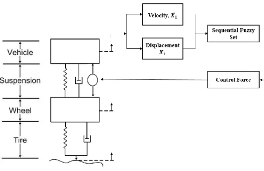
Figure 5 illustrates the model of the suspension system and control system. For the purposes of this thesis, a quarter car model was used. The design goal for this system is to stabilize and improve the response of the suspension. This is accomplished by measuring the velocity and position of the quarter-car mass, using them as inputs to a sequential fuzzy logic set to calculate the force used to dampen the suspension. Overall, the system is modeled as a second-order differential equation of forced damped vibration. The equation for current quarter car model can be written as shown in equations (12) and (13).

𝑚1𝑥̈1 = −𝑏1(𝑥̇1− 𝑥̇2) − 𝑘1(𝑥1− 𝑥2) + 𝑢 (12) 𝑚2𝑥̈2 = 𝑏1(𝑥̇1− 𝑥̇2) + 𝑘1(𝑥1− 𝑥2) + 𝑏2(𝑤̇ − 𝑥̇2) + 𝑘2(𝑤 − 𝑥2) − 𝑢 (13)

(31)

31

As per Dorf, Richard C., and Robert H. Bishop [35], equation (12) and (13) can be transformed into state-space equations shown in equations (14) and (15). A state-space model gives easier accessibility to multiple variables and is easily modelled in Simulink.

𝒙̇ = Ax + Bu……… (14) y = Cx + Du……… (15) Here, State Vector, x = [ 𝑥₁ 𝑥₂ 𝑥₃ 𝑥₄ ] Input signals, u =[ 𝑤 𝑤̇ 𝑢 ] where, 𝑥1 = 𝑥1 𝑥₂ = 𝑥̇₁ 𝑥₃ = 𝑥₂ 𝑥₄ = 𝑥̇₂

Now arranging the equation of 𝑥̇₁, 𝑥₁, 𝑥̇₂, 𝑥̈₂ in terms of 𝑥₁, 𝑥₂, 𝑥₃, 𝑥₄, 𝑢, 𝑤 and 𝑤̇ yields:

𝑥̇₁ = 𝑥₂ (16) 𝑥̇₃ = 𝑥₄ (17) 𝑥̇2 = 𝑥̈1 = −𝑏1(𝑥̇1−𝑥̇2)−𝐾1(𝑥1−𝑥2)+𝑢 𝑚1 So, 𝑥̇₂ = −𝑏1 𝑚1(𝑥2− 𝑥4) − 𝑘1 𝑚1(𝑥1− 𝑥3) + 𝑢 𝑚1 (18) 𝑥̇4 = 𝑥̈2= 𝑏1(𝑥̇1−𝑥̇2)+𝐾1(𝑥1−𝑥2)+𝑏2(𝑤̇−𝑥̇2)+𝐾2(𝑤−𝑥2)−𝑢 𝑚2

(32)

32 Then, 𝑥̇4 = 𝑏1 𝑚2(𝑥2− 𝑥4) + 𝑘1 𝑚2(𝑥1− 𝑥3) + 𝑏2 𝑚2(𝑤̇ − 𝑥4) + 𝑘2 𝑚2(𝑤 − 𝑥3) − 𝑢 𝑚2 (19) From equation (16) to (19), A = [ 0 1 0 0 −𝑘1 𝑚1 − 𝑏1 𝑚1 𝑘1 𝑚1 𝑏1 𝑚1 0 0 0 1 𝑘1 𝑚1 𝑏1 𝑚1 −𝑘1−𝑘2 𝑚2 −𝑏1−𝑏2 𝑚2 ] B = [ 0 0 0 0 0 1 𝑚1 0 0 0 𝑘2 𝑚2 𝑏2 𝑚2 −1 𝑚2] C = [ 1 0 0 0 0 1 0 0 0 0 1 0 0 0 0 1 ] D = [ 0 0 0 0 0 0 0 0 0 0 0 0 ]

Sequential Fuzzy Logic is used to calculate the commanded force in the model. The model uses vertical velocity and displacement of suspension as inputs to calculate actuator force. For fuzzy logic, a Mamdani Type Fuzzy Interference set was used [36], because Mamdani set rules can be developed from human experience in an easy to use linguistic form.

3.1.1. Quarter Car Model

The modeling parameters for the quarter car are similar to those in the work of Alleyne, Andrew, and Rui Liu[37] and modified within practical limits. Initially, the data was as shown in Table 1.

Table 1: Quarter Car Properties

Quarter Car Tire and Wheel

m1 = 250 kg m2 = 25 kg

b1 = 1,500 N/ms b2 = 600 N/ms

(33)

33

The system was simulated using Matlab and Simulink. The Simulink model consists of a quarter-car model and a fuzzy logic controller. The input for the fuzzy logic system’s rule set is the suspension deflection and the velocity. The main goal of the system is to minimize the vibration by controlling the rate of change in the suspension deflection.

To test the controller effectiveness, it was simulated with a disturbance input of a regular bump in the road, a large pothole, and a rough road profile. Each condition was tested independently and were combined for a final test.

The bumps in the road were simulated using two-different step functions, each lasting one second. The peak of the first step function was 6 cm and the second one was 10 cm (Figure 6a). For a large pothole, a sinewave of 6 cm amplitude and 1 rad/sec frequency was used, that lasted for 5.13 seconds (Figure 6b). To simulate the continuous disturbance of a rough road, a sine wave of 2 cm amplitude and frequency of 15 rad/sec was present throughout the simulation runtime (Figure 7a).

To accommodate various disturbances, the input fuzzy logic set was adjusted to give an appropriate range based on the movement range and limitations of the physical system. The output corresponding to the applicator force was selected with the goals of stability and practicality. Based upon the expected disturbances from the road, physical parameters of the system (spring and dampening coefficients) were adjusted.

(34)

34

Figure 6 (a): Road Bumps Figure 6 (b): Bump and Pothole A road bump is simulated by a step function (Figure 6a) to represent a sudden obstacle and associated rise and fall vertically. Figure 6b depicts the disturbance of a pothole, which is simulated with a portion of a high-amplitude sine wave. A continuous sine wave with low amplitude was picked to model a rough road as shown in Figure 7a. Finally, a combined disturbance was used (Figure 7b) as the worst scenario for tuning the initial fuzzy system.

Figure 7 (a): Rough Road Figure 7 (b): Combined Road Disturbance Figure 7b shows the combined disturbance, which is simulated for a duration of 35 seconds. In this combined disturbance, the rough road signal was present for the entire 35 seconds, the road

(35)

35

bump signal was present for 1 second starting at 6 and 10 seconds of simulation time, and the pothole signal was present between 20 to 25 seconds of simulation time.

3.2. Fuzzy Inference System (FIS) Development

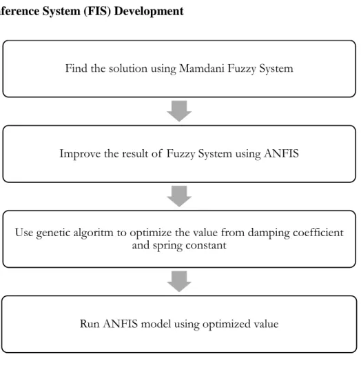
Figure 8: Steps in development of system

Fuzzy inference systems (FIS) are also known as fuzzy-rule-based systems, fuzzy models, or fuzzy controllers when used as controllers. An FIS consists of five parts as seen in Figure 9a [22]:

i. Rule Base - contains fuzzy rules in if-then format

ii. Database - contains membership function information including shape and value iii. Decision Making Unit - performs the rule inference operation

iv. Fuzzification Inference Unit - converts crisp input into fuzzy linguistic parameter Find the solution using Mamdani Fuzzy System

Improve the result of Fuzzy System using ANFIS

Use genetic algoritm to optimize the value from damping coefficient and spring constant

(36)

36

v. Defuzzification Inference Unit - converts fuzzy value into crisp output

Figure 9 (a): Block diagram of Fuzzy Inference System

(37)

37

Figure 9a shows a block diagram of an FIS, and Figure 9b shows a system comprised of two sequential FIS.

3.2.1. Development of Sequential Fuzzy Logic

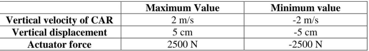
For the fuzzy logic controller, two different fuzzy sets were used to form a sequential fuzzy system. The first fuzzy set covered most cases and worked for a large range. The second fuzzy set worked when the magnitude of vibration attenuated to a lower range. This improved control of the system at important phases, allowing rules to be more compartmentalized and easier to work with. Both fuzzy sets take vertical velocity and displacement of the car as inputs and output the desired actuator force to control the vibration. Triangular membership functions were used for velocity, displacement, and force. For larger primary fuzzy set, five input membership functions were used for velocity and displacement and seven-output membership function were used for force. This gave the system sufficient freedom in controlling the vibration. The range for the parameters is shown in Table 2 and the rule matrix is shown in Table 3.

Table 2: Larger Range Fuzzy Set Parameters

Maximum Value Minimum value Vertical velocity of CAR 2 m/s -2 m/s

Vertical displacement 5 cm -5 cm

Actuator force 2500 N -2500 N

The parameter values used for velocity and displacement are based on Sharma et al [16] but the parameter for the actuator is based on an industrial linear actuator with push load of 2500N [38], the reason for picking this actuator parameter is size and force capability. An actuator with a higher force capability would have been better to control the vibration but too bulky to use in a standard car suspension. The rule matrix for the larger fuzzy set is shown in Table 3.

(38)

38 Table 3: Larger fuzzy membership table

Disp Vel NL N Z P PL NL PLL PLL PL P Z N PLL PL P Z N Z PL P Z N NL P P Z N NL NLL PL Z N NL NLL NLL

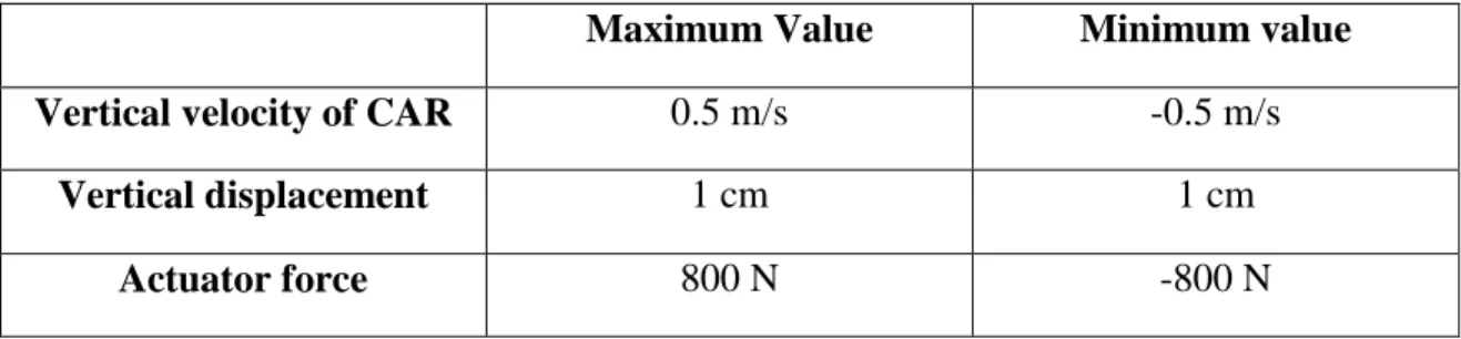
The smaller fuzzy set was used to provide finer control in the central portion of larger fuzzy set and have a smaller range of parameters as seen in Table 4. The design of the smaller fuzzy set was more focused and decision about the parameters were made using trial and error method, observing which values performed best. The chosen rule matrix for the smaller fuzzy set is shown in Table 5.

Table 4: Smaller Range Fuzzy set parameters

Maximum Value Minimum value Vertical velocity of CAR 0.5 m/s -0.5 m/s

Vertical displacement 1 cm 1 cm

Actuator force 800 N -800 N

Table 5: Smaller fuzzy membership table

Disp Vel N Z P

N PL P Z

Z P Z N

(39)

39

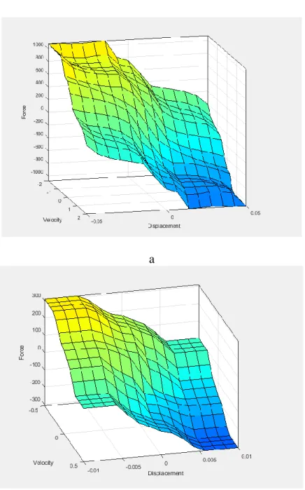
The resultant surface plots for both fuzzy sets are shown in Figure 9. It can be seen that the the larger is less linear, which allows it to compensate for different type of disturbance in ranges near the limits of the actuator. The smaller fuzzy set is more linear in nature but still applies a higher gain for small imputs.

a

b

(40)

40

3.3. Adaptive Neuro Fuzzy Inference System (ANFIS) Development

For an ANFIS, offline training is performed using the same data that used to develop Mamdani FIS and is used to compare the performance change between FIS and ANFIS system. and were tuned using Neural learning. Given the difficult in designing with gaussian membership functions, they are often not chosen; however, given the advantages of using a neural network, the shape of the membership functions were changed from triangular to gaussian prior to being tuned by the neural network.

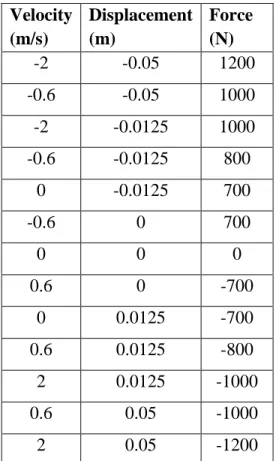
Table 6 shows the training data used, providing both the input and and the desired output . This data was used by the Neuro-Fuzzy Design tool in MATLAB to tune the membership functions.

Table 6: Training data for Neuro-Fuzzy System.

Velocity (m/s) Displacement (m) Force (N) -2 -0.05 1200 -0.6 -0.05 1000 -2 -0.0125 1000 -0.6 -0.0125 800 0 -0.0125 700 -0.6 0 700 0 0 0 0.6 0 -700 0 0.0125 -700 0.6 0.0125 -800 2 0.0125 -1000 0.6 0.05 -1000 2 0.05 -1200

(41)

41

For this study a combined hybrid model using both LSE and gradient descent methods (as described earlier) was used to train the fuzzy system. The resultant rule set increased the system performance within the restriction of parameters. Below in Figure 11, the change of membership function due to neural learning is shown. The training error for each epoch/iteration of the training is shown in Figure 12. It can be seen that the system converged after 3 epochs using the hybrid method compared to back-propogation method, which failed to converge after 1000 epochs. Clearly, the Hybrid Neural Learning method converged faster resulting in a low error of 0.0013 after 10 epoch whereas with back propagation method maintained a high error of 872.61 after 1000 epochs.

Figure 11 (a): Membership function for displacement before Neural Training

Figure 11 (b): Membership function for displacement after Neural Training

(42)

42

Figure 12 (a): Training error using Hybrid Neural Learning

Figure 12(b): Training error using back-propagation neural learning

Figure 13 shows a comparison of membership functions between regular FIS and ANFIS. In addition to changes in the membership function shape, there were also changes to the range. The changes in the membership finctions can also be seen in Figure 14, which depicts the FIS

(43)

43

surface before and after training with a neural network. The main difference between the two is the high gain (shown as a steep surface) in the middle associated with the displacement input.

Fuzzy Neuro Fuzzy

a d

b e

c

Figure 13: Membership function for Fuzzy and Neuro Fuzzy System.

a) Input displacement (Fuzzy) b) Input velocity (Fuzzy) c) Output force (Fuzzy)

d) Input displacement (Neuro Fuzzy) e) Input velocity (Neuro Fuzzy)

(44)

44 a

b

(45)

45

3.4. Optimization Through Genetic Algorithms

To further improve the system, the damper and spring combinations were modified to provide improved performance for the car. This was done using a genetic algorithm. For this optimization problem, the damping co-efficient the limited to a range of 750-1800 and the spring constant was limited to a range of 12,000-18,000.

To begin, an initial random population was created within the limits. The size of the population was 50, and each member of the population is defined with two variables. For fitness function squared sum of force, F and displacement, X1 was taken at every 0.01 sec. So, for total 15 sec the data point was n=15/0.01=1500 . Total number of peaks, p was calculated from dampned displacement as shown in Figure 15 .

‘

(46)

46 The fitness function used is

F = 1 𝑛√∑ (𝐹𝑘∗ 𝑋𝑘) 2 𝑛 𝑘=1 ∗ (𝑝 − 𝐶) where 1 𝑛√∑ (𝐹𝑘∗ 𝑋𝑘) 2 𝑛

𝑘=1 is the RMS (Root Mean Square) of the work on the quarter-car mass, p is the number of peaks in the vibration, and C is a constant chosen based on the number of expected oscilations. For ride stability, three parameters were considered: the amount of displacement, force applied, and frequency. Force and displacement is combined into actuator work. Works done is related to the performance of the actuator, which in turns is related to stability of ride and logivity of suspension system. So, one main goal was to minimize the work done by the actuator but keep the vibration dampened. Additionally, the frequency of vibration is also related to ride comfort, so lower frequency was preferred to higher, and it was seen that the number of waves in different scenario varies between 36-48. To penalize the high frequency vibration, a constant value (C=35) was used and subtracted from the number of waves and the difference was multiplied with RMS value of work done. With this fitness function, all criteria which contribute to the desired performace are accounted for and the genetic algorithm will work to minimize the value, finding the best balance.

In the genetic algorithm optimization, the crossover rate for the new generation was 0.8 and Mutation rate was 0.01. For crossover scattered function was used. This is a built in Matlab function where the child is created by taking a random part form each parent. Scattered creates a random binary vector. Scatter crossover select gene from first parent when binary value of random crossover vector 1 and gene from second parent if binary value is 0. For example: Lets take two individual with values of (1500, 15000) and (1200, 17000). If considering the first variable (dampening coeficiente) of the two individuals, 1500 and 1200, they can be presented in binary as

(47)

47

parent1(1500) = [10111011100] parent2(1200) = [10010110000]

If the given random crossover vector is [1 1 0 0 1 0 0 0 1 1 0] the resultant child value would be child = [10011110100], which is decimal 1268.

For mutation, the adaptive feasible function is used to keep the resultant child within the range specified. The adaptive feasible function randomly generates directions that are adaptive with respect to the last successful or unsuccessful generation. A built-in Matlab function is used for the adaptive mutation, where a step length was chosen to progress the evolution in each direction so that bounds are satisfied.

(48)

48

4. Results & Discussion

FIS system:

Initially, a sequential FIS model was used to calculate the force for the actuator. As seen in Figure 16, the overall response of the system against high frequency low amplitude wave (rough road ) was not satisfactory as the displacement remains attenuated to a large extent; however, the actuator with FIS controller did perform well with the road bump at 6 seconds. Further comparison of the system performance can be seen in Figure 17, which compares the performance of the system with and without the actuator. The figure shows that the system with the actuator performed better than the basic spring damper system without an actuator.

(49)

49

Figure 17: Displacement of QCM mass with FIS controlled actuator and without any actuator Under FIS the system was damping vibration generated by sudden bump, but in scenario with bump with larger disturbance which is out of preset parameter of fuzzy set; the force was inadequate to control the damping. Also, we can see controller fails to make adjustment when the larger disturbance that is out of range was applied. There was no controlling force (Figure 18) between 10-12 sec, this is due to disturbance is out of range for fuzzy set and the controller fails to adjust accordingly. Also, even though system was able to control the continuous disturbance of high frequency, to a degree the result was not good enough.

(50)

50

Figure 18: Force under FIS system

ANFIS performance:

With new rule base generated with Neural learning, the dampened vibration has comparatively lower amplitude and overall improved performance as shown in Figure 18. In Figure 19, it can be seen that the force applied is comparatively lower with ANFIS model, the only exception is when there is larger disturbance that is out of our specified limit. Consequently, the ANFIS model can adapt and apply a higher force gain to control the vibration more effectively in this scenario. This can be seen in Figure 19 that even when vertical displacement is out of range between 10-12 sec, ANFIS model can infer higher force (Figure 20) and by applying that force, vibration is getting damped better compared to FIS model.

(51)

51

Figure 19: Comparison of Displacement with ANFIS and with FIS

(52)

52

ANFIS with Optimized with Genetic Algorithm (GA) Parameter:

The GA used an initial population of 50, and the optimization was set to run for 100 generations with stalling criteria set at 5 generations. With multiple run the solution always converged between 12-14 generation, example from the best run is shown in Figure 21.

Figure 21: Convergence of Optimization

Even the solution was set to run for 100 generations, stalling criteria with function tolerance of 1e-6, which triggered an early termination as shown in Figure 22.

(53)

53

The result from three different runs are shown in Table 7. All the results are close in magnitude. The results shown are from the best optimization run.

Table 7: Results from GA Optimizations

Run No of generation b1 k1 fitness

1 13 812.602 12168.59 1.01506

2 12 845.49 12346.79 1.0338

3 14 822.961 12297.37 1.01325

From random run of 100 different samples of b1 and k1, the best value was b1= 1062.95 and k1=12372.408, resulting in Fitness = 1.12911. The fitness values for 100 random runs is shown in Figure 23 (all the data of random run is in appendix B). The fitness values from all 100 radomly generated systems (set of b and k) were worse (higher) than every GA run. From Table 7 and Figure 23, it is evident that genetic algorithm optimization provided an improved fitness value by 11.4% compared to best result from random run. The optimization tended to converge within 13 generations, ending with the stall criteria (one exception was 22 generation). For all the optimization runs the final fitness value was always comparable, highest and lowest valued best fitness was within 2% of each other.

(54)

54

Figure 23: Fitness value from 100 random run

Figure 24: Displacement comparison between GA optimized ANFIS and ANFIS

Figure 24 shows that the relative performance of the system after the optimization of the spring and damper. It can be seen that optimized damper and spring value perform better in bump,

1 1.2 1.4 1.6 1.8 2 2.2 2.4 2.6 2.8 3 0 10 20 30 40 50 60 70 80 90 100 Fi tn e ss V al u e Run no

(55)

55

but everywhere else damping performance of regular damper and spring under ANFIS is unchanged.

Figure 25: Force comparison between GA ANFIS and ANFIS

Figure 25 shows a comparison of the force used by the actuator before and after the optimization. The force required for the optimized ANFIS is consistently lower during rough road period. To better show the performance difference Figure 26 focusses on the results from 5 to 12 seconds; the amplitude of displacement under optimized physical parameter is clearly lower than the displacement with the original parameters.

(56)

56

Figure 26: Displacement comparison between GA ANFIS and ANFIS time 5 to 12 sec

Figure 27: Force comparison between GA optimized ANFIS and FIS

Finally, the force utilization of FIS system and ANFIS system with GA optimization is compared in Figure 27. It can be seen that the optimized ANFIS system utilizes much less force, which is beneficial for actuator health, performance, and energy usage. It can be concluded that

(57)

57

the FIS system with actuator control improved performance of the basic spring damper system, but basic FIS system design methods have limitations which can be overcome by using a neural network to train the membership function. Finally using GA optimization for spring and dampner can further improve the response of the system to a forced vibration with lower force required for the actuator.

(58)

58

5. Conclusion

In this thesis, an active vibration control method was developed for automotive suspension. The model was tested against a quarter car model that was represented using a state-space model. The force required to control the vibration actively was calculated using FIS model. The result was inadequate for few cases, so the system was further improved by the development of an adaptive neuro fuzzy model. The ANFIS model was trained with a hybrid of least square and the gradient method. The training with the hybrid approach converged very fast within few epochs and error was within the order of 1/1000. When only training with regular back propagation, the convergence was slow, and error was high. For example, at 1000 epoch the error was about at 872 with back propagation.

To further improve results, a genetic algorithm was used to optimize the model parameters of the system. A bounded, continuous search space was defined for the critical parameters of damping coefficient and spring constant of the suspension. The fitness function was based on actuator energy and frequency of vibration. Finally, the optimization result was compared with a random search space to verify the effectiveness of GA. It is found that result from GA yielded a better fitness compared to best result of random runs. That indicates GA optimization was successful in finding a solution.

In future work, instead of a quarter car model, a whole car model can be used to test more accurately and to reflect the complexity of a whole car suspension. Additionally, optimizing the basic spring damper system before using actuator with either of FIS or ANFIS controller may produce different results. The GA optimization population sample can be increased along with stall criteria to run the GA optimization longer and see if there is further improvement of result.

(59)

59

The GA could also be used to optimize additional variables, including the fuzzy controller. The system was simulated using Simulink to determine the fitness; this is computationally heavy. Alternative methods of calculating the fitness can be explored. Additionally, rather than using the generated disturbances used in testing, real road data can be used as an alternative to more accurately reflect real-life road conditions. Finally, whole model can be experimentally tested for further improvement, main challenge there will be the actuator, even though comparable actuator with required weight and force capacity is already available, their reaction time is slow for an effective active vibration control; however, it can be inferred from the results that the proposed ANFIS model for vibration control is effective and GA optimization provides further control performance within practical search space for physical parameters.

To summarize, an active vibration control for suspension was studied using a quarter car model. Intially FIS controller is used to calculate force required for actuator, which improved the performance for a road bump, but struggled in continuous rough road disturbances. Then ANFIS was used to train and modify the membership functions, leading to substantial increase in performance with both rough road and bump disturbances. Finally, the basic suspension was optimized using GA, which led to additional performance gains.

(60)

60

Appendices

Appendices A: Sample calculation of a Fuzzy Inference system

Let’s a consider the FIS system used in this thesis. The system has 2 input:

Distance (5 level): NL, N, Z, P, PL ; Speed (5 level): NL, N, Z, P, PL 1 output:

Force (7 level): NLL, NL, N, Z, P, PL, PLL Few examples of rules:

If (Velocity is Z) and (Displacement is Z) then (Force is Z)

If (Velocity is Z) and (Displacement is NL) then (Force is PL)

Now For a single test case of velocity (V) of -0.2 m/s and displacement (D) of -4 cm first the input V and D are fuzzified.

Fuzzification:

Here, by definition and according to figure 28, V is subset of both N and Z ; D is subset of both NL and N.

(61)

61

Rule base:

Now for fuzzy values of V and D 4 different rule is triggered and each results a different fuzzy output.

Rule triggered in this case are:

 If (Velocity is Z) and (Displacement is NL) then (Force is PL)

 If (Velocity is N) and (Displacement is NL) then (Force is PLL)

 If (Velocity is Z) and (Displacement is N) then (Force is P)

 If (Velocity is N) and (Displacement is N) then (Force is PL) It can be seen in last blue column of figure 11.

Defuzzification:

Defuzzifications first combines all the fuzzy actions into one action. Then transform said action into a crisp vale. As can be seen in figure 29.

(a)

(b)

Figure 29: Surface Plot for (a) Combined output area, (b) Combined output with COG (red mark) In this work center of gravity (COG) is used to calculate the crisp value. the resultant crisp force is 1366 N.

(62)

62

Appendices B:

Table 8: Fitness data from 100 randomly generated damping co-efficient and spring constant

Sample No Damping coefficient, b1 Spring constant, k1 Fitness value

1 1307.349 14941.703 1.95361 2 1241.608 13283.9 1.63453 3 1279.535 12238.746 1.52045 4 957.692 12346.285 1.39405 5 822.849 18175.934 1.66977 6 1271.121 14378.246 1.45121 7 1462.667 12258.346 1.91437 8 1079.058 14861.688 1.75343 9 1324.138 17963.999 2.49711 10 890.154 15673.233 2.17602 11 1084.19 16847.348 1.8603 12 1282.024 17660.15 2.46784 13 957.019 17097.77 1.90256 14 1241.324 13219.588 1.59165 15 839.248 15737.73 2.2137 16 1469.808 14552.893 2.29201 17 1188.951 13678.59 1.68399 18 1313.45 13913.213 1.7723 19 1129.468 17243.075 1.94396 20 1418.177 19194.686 2.66134 21 1160.412 13039.683 1.56551 22 861.971 13931.312 1.73081 23 1380.538 13907.116 2.14873 24 1360.714 13826.437 2.11868 25 1446.948 14624.878 2.29214 26 897.446 13883.129 1.69174 27 1212.034 15549.666 1.64254 28 1013.745 18231.215 2.14921 29 1188.948 16122.927 1.74654 30 1437.895 14143.793 2.22237 31 1317.9 17652.968 2.42623 32 1035.334 16258.662 1.72754 33 806.891 12404.626 1.28575 34 1148.098 17843.754 2.03894 35 1450.508 12974.297 2.01244 36 1176.618 15520.43 1.63649 37 758.927 14528.42 1.90432

(63)

63 38 871.637 17957.134 1.58871 39 983.411 15963.999 1.99483 40 874.237 16514.865 1.64241 41 947.228 16905.593 1.83604 42 1266.911 17611.137 2.47218 43 1087.906 12628.66 1.46228 44 921.733 18850.03 2.3783 45 864.284 18193.627 1.64653 46 1153.757 19471.01 2.88902 47 808.632 15320.087 2.07156 48 829.99 19214.236 1.90974 49 753.476 17811.828 2.1766 50 1362.977 18515.21 2.57118 51 813.327 14998.37 1.99625 52 944.903 18000.514 2.11909 53 1073.56 18829.857 2.25746 54 886.385 13978.522 1.80245 55 859.154 13020.514 1.67709 56 1401.969 16347.784 2.62882 57 1162.395 13087.161 1.58856 58 1389.773 16665.413 2.71153 59 1013.214 15849.372 2.0493 60 1051.356 12569.75 1.4207 61 929.937 12924.892 1.69166 62 887.931 13799.644 1.72984 63 1062.95 12372.408 1.12911 64 1427.037 19085.904 2.63508 65 1118.148 15669.395 1.6358 66 1003.29 18750.404 2.28589 67 1026.935 12834.021 1.96021 68 1335.189 14923.041 1.93281 69 931.268 15029.341 2.2648 70 822.341 12989.8 1.34096 71 1456.538 19171.009 2.62999 72 1181.406 12448.347 1.50154 73 926.085 14648.689 2.35638 74 1365.896 12115.526 1.78855 75 782.268 13267.425 1.59915 76 1236.837 17487.918 2.43018 77 1235.809 15381.928 1.60796 78 1160.257 14222.406 1.73239 79 1308.52 13417.163 1.34156 80 1265.082 13376.334 1.54591

(64)

64 81 1026.363 16692.139 1.82575 82 1335.171 12608.443 1.8647 83 1447.039 17817.845 2.89585 84 1115.094 15268.939 1.56367 85 1085.088 14297.621 2.32937 86 1131.381 15830.787 1.66328 87 1363.221 17961.236 2.4854 88 1233.239 14839.57 1.53767 89 1358.685 15996.192 2.12198 90 1013.045 19042.512 2.36616 91 1406.957 16126.173 2.59157 92 1216.856 16402.835 1.78004 93 905.807 14259.347 1.8194 94 1103.193 13728.661 1.65614 95 1383.232 13460.732 2.06519 96 919.441 13280.31 1.93904 97 920.748 15267.74 2.39168 98 983.327 18925.347 2.34186 99 1072.656 13386.122 1.89297 100 1428.661 19348.113 2.66395 Best (Fitness) 1062.95 12372.408 1.12911 Worst (Fitness) 1447.039 17817.85 2.89585 Median (Fitness) 829.99 19214.24 1.90974