MODELING OUT-OF-ORDER SUPERSCALAR
PROCESSOR PERFORMANCE QUICKLY AND
ACCURATELY WITH TRACES
by
Kiyeon Lee
B.S. Tsinghua University, China, 2006
M.S. University of Pittsburgh, USA, 2011
Submitted to the Graduate Faculty of
the Dietrich School of Arts and Sciences in partial fulfillment
of the requirements for the degree of
Doctor of Philosophy
in
Computer Science
University of Pittsburgh
2013
UNIVERSITY OF PITTSBURGH
DEPARTMENT OF COMPUTER SCIENCE
This dissertation was presented
by
Kiyeon Lee
It was defended on
August 12th 2013
and approved by
Sangyeun Cho, Ph.D., Associate Professor at Department of Computer Science
Rami Melhem, Ph.D., Professor at Department of Computer Science
Youtao Zhang, Ph.D., Associate Professor at Department of Computer Science
Alex K. Jones, Ph.D., Associate Professor at Electrical and Computer Engineering
Dissertation Director: Sangyeun Cho, Ph.D., Associate Professor at Department of
MODELING OUT-OF-ORDER SUPERSCALAR PROCESSOR PERFORMANCE QUICKLY AND ACCURATELY WITH TRACES
Kiyeon Lee, PhD
University of Pittsburgh, 2013
Fast and accurate processor simulation is essential in processor design. Trace-driven simu-lation is a widely practiced fast simusimu-lation method. However, serious accuracy issues arise when an out-of-order superscalar processor is considered. In this thesis, trace-driven sim-ulation methods are suggested to quickly and accurately model out-of-order superscalar processor performance with reduced traces. The approaches abstract the processor core and focus on the processor’s uncore events rather than the processor’s internal events. As a result, fast simulation speed is achieved while maintaining fairly small error compared with an execution-driven simulator. Traces can be generated either by a cycle-accurate simulator or an abstract timing model on top of a simple functional simulator. Simulation results are more accurate with the method using traces generated from a cycle-accurate simulator. Faster trace generation speed is achieved with the abstract timing model. The methods determine how to treat a cache miss with respect to other cache misses recorded in the trace by dynamically reconstructing the reorder buffer state during simulation and honoring the dependencies between the trace items. This approach preserves a processor’s dynamic uncore access patterns and accurately predicts the relative performance change when the processor’s uncore-level parameters are changed. The methods are attractive especially in the early design stages due to its fast simulation speed.
TABLE OF CONTENTS
1.0 INTRODUCTION . . . 1
1.1 Problem definition . . . 2
1.2 Overview of the approach . . . 5
1.3 Thesis contributions . . . 8
1.4 Thesis organization. . . 9
2.0 BACKGROUND . . . 10
2.1 Out-of-order superscalar processor . . . 10
2.2 Performance modeling methods . . . 13
2.2.1 Trace-driven simulation . . . 16
2.2.2 Analytical models for out-of-order superscalar processors . . . 18
2.2.3 Other simulation time reduction techniques . . . 20
3.0 TRACE SIMULATION WITH TIMING INFORMATION . . . 24
3.1 Overview . . . 24
3.2 Model 1: Isolated Cache Miss Model . . . 25
3.2.1 Basic idea . . . 25
3.2.2 Instruction permeability analysis . . . 26
3.2.3 Experimental setup . . . 28
3.2.4 Evaluation result . . . 29
3.3 Model 2: Independent Cache Miss Model. . . 32
3.3.1 Basic idea . . . 32
3.3.2 ROB occupancy analysis in the independent cache miss model . . . . 33
3.4 Model 3: Pairwise Dependent Cache Miss Model (PDCM) . . . 35
3.4.1 Basic idea . . . 35
3.4.2 Preparing reduced trace in PDCM . . . 36
3.4.3 ROB occupancy analysis in PDCM . . . 37
3.4.4 Modeling a superscalar processor . . . 38
3.4.4.1 Reconstructing the ROB . . . 38
3.4.4.2 Out-of-order trace simulation . . . 39
3.4.4.3 Simulation algorithm of PDCM . . . 42
3.4.4.4 Modeling various processor artifacts in PDCM . . . 45
3.4.5 Experimental setup . . . 47
3.4.6 Evaluation result . . . 49
3.4.6.1 Accuracy of PDCM . . . 49
3.4.6.2 Reproducing temporal uncore access behavior . . . 56
3.4.6.3 Predicting the performance with different uncore parameters . 58 3.4.6.4 Simulation speed and storage requirements of PDCM . . . 62
3.5 Summary . . . 63
4.0 TRACE SIMULATION WITH ABSTRACT TIMING INFORMATION 65 4.1 Overview . . . 65
4.2 Trace generation in In-N-Out . . . 66
4.2.1 Data dependency in superscalar processor . . . 67
4.2.2 Memory dependency in superscalar processor . . . 69
4.2.3 Microarchitectural dependency in superscalar processor . . . 71
4.2.4 Dependence-graph model . . . 72
4.2.5 Trace generation algorithm in In-N-Out . . . 75
4.3 Trace simulation in In-N-Out . . . 78
4.3.1 ROB occupancy analysis in In-N-Out . . . 78
4.3.2 Simulation algorithm of In-N-Out . . . 80
4.3.3 Modeling various processor artifacts in In-N-Out . . . 85
4.4 Experimental setup. . . 88
4.5.1 Accuracy of In-N-Out . . . 88
4.5.2 Impact of uncore components . . . 97
4.5.3 Simulation speed and storage requirement . . . 101
4.6 Summary . . . 102
5.0 COMPARING PDCM AND IN-N-OUT . . . 103
5.1 Comparing the accuracy . . . 103
5.2 Case Study . . . 106
5.3 Limitations of PDCM and In-N-Out . . . 110
6.0 CONCLUSIONS . . . 111
7.0 FUTURE RESEARCH DIRECTION . . . 114
7.1 Trace-driven simulation for multi-core processors . . . 114
7.1.1 Multicore system model . . . 115
7.1.2 Goals . . . 115
7.1.3 Evaluation methods . . . 116
LIST OF TABLES
1 Comparing different performance modeling methodologies. . . 14
2 Various techniques to reduce the simulation time. . . 20
3 The baseline machine configuration for evaluating the isolated cache miss model. . 28
4 Inputs for the SPEC2K benchmarks. . . 29
5 Notations used for the PDCM algorithm description. . . 39
6 Baseline and realistic superscalar processor configurations to evaluate PDCM. . . 48
7 The accuracy ofPDCM with different processor core configurations. . . 51
8 The percentage of stable branch instructions in the benchmarks. . . 53
9 The average, minimum, and maximum CPI errors of PDCM observed throughout a program execution using the realistic configuration. . . 56
10 The similarity in memory access patterns betweensim-outorderand PDCM. . . . 60
11 The relative CPI differences betweensim-outorderand PDCM. . . 61
12 The dependencies (edges) depicted in the dependence-graph model. . . 73
13 The weight on edges between the nodes in the dependence-graph model. . . 74
14 Notations used for the In-N-Out algorithm description.. . . 80
15 The accuracy ofIn-N-Outwith different processor core configurations. . . 90
16 The average, minimum, and maximum CPI errors ofIn-N-Outobserved throughout a program execution using the realistic configuration. . . 95
17 The similarity in memory access patterns betweensim-outorderand In-N-Out. . 99
18 The relative CPI difference betweensim-outorder and In-N-Out. . . 100 19 Absolute CPI errors ofPDCM and In-N-Outusing different machine configurations. 104
LIST OF FIGURES
1 Inaccurate CPI results from a na¨ıve trace-driven simulation of a superscalar
proces-sor. . . 4
2 A high-level view of a trace-driven simulation method. . . 6
3 Machine model having a superscalar processor core, L2 cache, and main memory. 11 4 Overall structure of PDCM. . . 25
5 The basic idea of the isolated cache miss model. . . 26
6 Experiment results with the isolated cache miss model.. . . 31
7 An example of ROB occupancy analysis in the independent cache miss model.. . . 33
8 The CPI errors of the independent cache miss model when the ROB size is 64. . . 35
9 An example of ROB occupancy analysis in PDCM. . . 37
10 An example of out-of-order trace simulation. . . 41
11 High-level pseudo-code of trace simulation in PDCM. . . 42
12 High-level pseudo-code for reconstructing the ROB. . . 44
13 High-level pseudo-code for processing a trace item. . . 45
14 Two observed aspects that can affect the accuracy of branch handling. . . 46
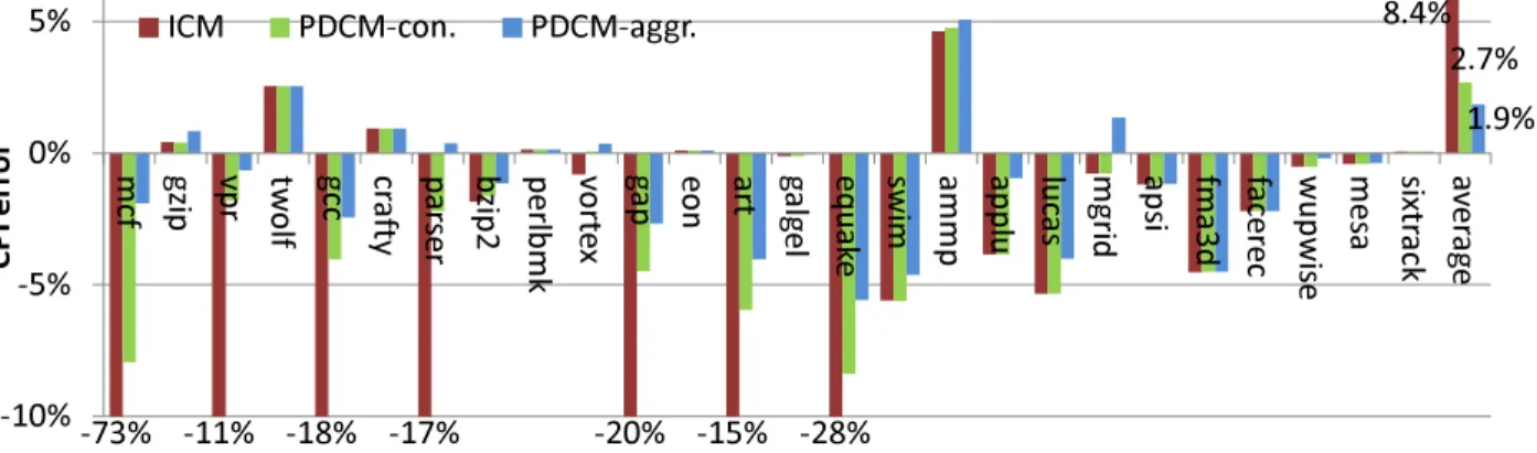
15 The CPI errors of the SPEC2K benchmarks using the baseline configuration inPDCM. 49 16 The CPI errors before (base) and after (base+real branch predictor) incorporating a realistic branch predictor inPDCM.. . . 52
17 The relative CPI changes with a tagged L2 data prefetcher inPDCM. . . 54
18 The relative CPI changes with a limited number of L2 MSHRs inPDCM. . . 54 19 The CPI errors of the SPEC2K benchmarks using the realistic configuration inPDCM. 55
20 The change in CPI oflucasshown bysim-outorder and PDCM while simulating 1B
instructions (1,000 intervals). . . 57
21 The temporal off-chip access pattern ofPDCM compared with sim-outorder. . . . 60
22 The relationship between the simulation speed and trace file size inPDCM. . . 63
23 Overall structure of In-N-Out. . . 66
24 An example of instruction data dependency in a program. . . 67
25 An example of eight instructions constituting two dependency chains. . . 69
26 An example of a memory dependency in a program. . . 70
27 The dependence-graph model with four instructions. . . 73
28 An example of collecting the abstract timing information using the dependence-graph model in trace generation.. . . 74
29 The high-level pseudo-code of the trace generation algorithm. . . 77
30 An example of ROB occupancy analysis in In-N-Out. . . 79
31 The high-level pseudo-code of the trace simulation algorithm. . . 81
32 High-level pseudo-code for committing trace items. . . 82
33 High-level pseudo-code for updating the ROB. . . 83
34 An example of estimating the dispatch time of trace items in trace simulation. . . 83
35 The high-level pseudo-code for MSHR allocation. . . 85
36 The high-level pseudo-code for modeling the instruction caching effect. . . 87
37 The CPI errors of the SPEC2K benchmarks using the baseline configuration in In-N-Out. . . 89
38 The CPI errors before (base) and after (base+real branch predictor) incorporating a realistic branch predictor inIn-N-Out. . . 92
39 The relative CPI changes when different L2 data prefetchers are used in In-N-Out. 93 40 The relative CPI changes with a limited number of L2 MSHRs inIn-N-Out. . . . 94
41 The CPI errors of the SPEC2K benchmarks using the realistic configuration in In-N-Out. . . 94
42 The change in CPI ofparsershown bysim-outorderandIn-N-Outwhile simulating 1B instructions (1,000 intervals). . . 96
44 The relationship between the simulation speed and trace file size inIn-N-Out. . . 101 45 A case study forPDCM and In-N-Out. . . 109 46 Target multicore machine model. . . 115
1.0 INTRODUCTION
As higher microprocessor performance is desired, the microprocessor design has evolved and achieved spectacular breakthroughs over the last decades. In the 1990s, the microproces-sor performance showed a significant boost with higher clock frequencies through deeper pipelines and advanced microarchitectural techniques, such as out-of-order execution and aggressive branch prediction [31, 67]. Computer architects have introduced architecture in-novations to increase the parallelism in various forms—instruction-level parallelism (ILP), memory-level parallelism (MLP), and the thread-level parallelism (TLP)—present in today’s microprocessors [31]. ILP is achieved by executing multiple instructions in parallel supported by multiple functional units and the multi-issue capability of a processor. MLP is achieved as an effect of ILP and the capability of the processor’s cache subsystem to issue and track mul-tiple outstanding requests to the main memory. In a single-core processor, TLP is realized by executing multiple threads simultaneously on a single multithreaded processor core.
Starting from the decade of 2000, the trend in microprocessor design changed from a single-core processor to a multicore processor architecture. Rather than squeezing the performance out of a single-core processor core, a multicore processor improves the system performance by increasing the total throughput of the system. In multicore architecture, TLP is realized by executing multiple threads simultaneously on multiple processor cores.
As more and more processor cores are integrated in a single chip, the performance of the underlying memory subsystem is critical to achieve high overall performance. More specifically, as the number of processor cores in a chip increases, the contention in the shared resources, such as the interconnection network, the last-level cache, and the memory controller, has a significant and growing impact on the performance of a multicore processor system. Such shared resources are sometimes referred to as “uncore” components [18, 64],
distinguished from the processor core components such as the branch predictor and the L1 caches.
Developing a microprocessor system involves a thorough evaluation of the processor per-formance, including the effect of advanced microarchitectural techniques like branch predic-tion and out-of-order instrucpredic-tion execupredic-tion, over several processor design stages. In the early design stages, when the target processor system is not available, computer architects rely on software simulation techniques with abstract performance models or rely on analytical models to quickly explore a large design space and study the design trade-offs. More detailed cycle-accurate execution-driven simulation, which closely models the events that occur in an actual processor, is required in the later design stages as the microprocessor design gets fi-nalized. After the silicon of a processor is available, the performance measurement units are used to measure the performance of the implemented processor system. The performance evaluation of a processor is a major challenge as it requires various tools, methodologies, and experience [4].
1.1 PROBLEM DEFINITION
Software simulation enables one to quickly analyze the behavior of a complex system and to evaluate subtle design trade-offs in a controlled experimental environment. However, despite all the advantages, simulation may be unacceptably slow. Simulating seconds of program execution in real time may entail days of simulation. This slow simulation speed affects the development progress of a new processor design. Hence, improving the simulation efficiency by increasing the simulation speed without sacrificing the simulation accuracy has been a hot research topic in the computer architecture community. It is particularly important to perform a fast and reasonably accurate simulation in early design stages.
Trace-driven simulation is a widely practiced simulation method when the traces are prepared and fast simulation is required [73,82]. To run a simulation, a trace of interesting
processor events1 need to be generated prior to simulation. Once the trace has been prepared it can be reused multiple times with different machine configurations. Replacing detailed functional execution with pre-captured trace results in a much faster simulation speed than an execution-driven simulation method. Thanks to its high speed, trace-driven simulation is especially favored in early design stages [73]. Unfortunately, the accuracy of trace-driven simulation has often been questioned when modeling a complex processor such as an out-of-order superscalar processor [10]; the static nature of the trace poses challenges when modeling a dynamically scheduled out-of-order superscalar processor2 [10, 43, 45]. As a result, trace-driven simulation has been typically limited to modeling relatively simple in-order processors, unless a full instruction trace of a program is available.
In contrast, execution-driven simulation is a simulation method used to simulate the behavior of a processor in detail without traces. It simulates the processor in a cycle-by-cycle basis which provides great flexibility to simulate a complex processor and returns accurate simulation results. To model a superscalar processor, it is believed that full tracing and computationally expensive detailed modeling of processor microarchitecture are required [4]. However, this comes with the cost of a long development time and a slow simulation speed. In this dissertation, accurate trace-driven simulation usingreduced traceis considered for modeling superscalar processor performance. The reduced trace only includes accesses to the uncore components, a subset of the entire instructions, and summarizes the instructions executed between operations. There are prior trace-driven simulation works using filtered trace[73], which is a trace of memory references filtered from the program instruction stream. In this dissertation, the notion of reduced trace is used to represent a trace of accesses to the uncore components obtained by filtering the L1 cache hits.
Filtered trace based simulation is desirable because filtered trace simplifies the complexity of modeling a processor core, obtains results faster, and requires less storage space than trace-driven simulation using full instruction traces. Trace-driven simulation with filtered trace works well for in-order processors. For example, consider the detailed simulation of a 1In this dissertation, a trace of a single processor event is denoted as a “trace item”. The size of a trace item depends on the amount of information stored in the trace item. It is usually in the range of several 10’s of bytes.
2In this dissertation, the terms “out-of-order superscalar processor” and “superscalar processor” are used interchangeably.
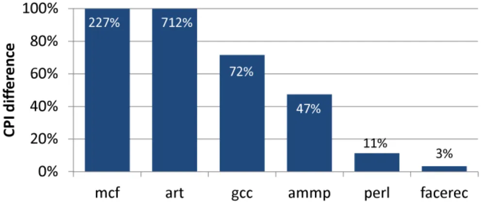
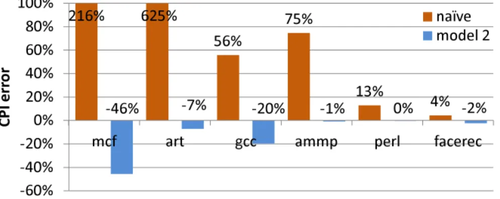
227% 712% 72% 47% 11% 3% 0% 20% 40% 60% 80% 100%
mcf art gcc ammp perl facerec
C P I d if fe re n c e
Figure 1: Inaccurate CPI results from a na¨ıve trace-driven simulation of a superscalar processor.
simple in-order processor. During the trace generation phase, one might record the type and the address of every memory operation as well as the number of instructions executed and the number of cycles elapsed since the last memory operation. Because the core executes instructions in order and blocks while waiting for a memory access, the filtered trace would be the same regardless of the memory configuration. Thus, using the same trace, one could simulate many different memory hierarchy configurations, such as different cache latencies or cache sizes, with high cycle accuracy and fast simulation speed.
However, this straightforward approach does not work for a superscalar processor, since it does not necessarily block during a long latency operation and executes other instructions to hide the latency cost. For example, a superscalar processor executes instructions during a long latency off-chip access to hide the cost of the long latency. Even multiple off-chip accesses can be simultaneously outstanding while the data fetched by individual access is still in transit from the memory. Moreover, the impact of an off-chip access on program execution time is determined dynamically during program runtime and changes with different machine configurations. However, a trace naturally contains the choices made by a core in one partic-ular instance of execution. Figure 1, produced using a typical 4-issue superscalar processor model and a selected set of benchmarks from the SPEC2K benchmark suite [70], shows that using the na¨ıve approach described above to model superscalar processor performance indeed results in very high errors.
It is not straightforward how to assess the impact of a memory access in a superscalar processor with pre-generated filtered trace, especially if one wants to further reduce the amount of trace for faster simulation speed. In this dissertation, practical and effective trace-driven simulation methods are developed and evaluated using reduced trace to model the performance of superscalar processors, especially when the focus of a study is on uncore components such as the L2 cache and the memory controller.
1.2 OVERVIEW OF THE APPROACH
Previously, researchers proposed analytical performance models to quickly derive the per-formance of superscalar processors [13, 24, 36, 52]. For example, Karkhanis and Smith [36] proposed a first-order analytical performance model to estimate a superscalar processor’s performance by paying attention to “miss events” that can stall program execution, such as branch misprediction, instruction cache miss, and data cache miss. The overall performance of a program is derived by adding the ideal CPI and the CPI increase due to the miss events. Chen and Aamodt [13] and Eyerman et al. [24] extended the first order model by improving its accuracy and incorporating more processor artifacts. Michaud et al. [52] built a simple analytical model based on the observation that the instruction-level parallelism (ILP) grows as the square root of the instruction window size. These analytical models derive the overall performance of superscalar processors from relatively simple mathematical models. How-ever, the mathematical models cannot reproduce (or simulate) the dynamic behavior of the processor being modeled. In this dissertation, I focus on trace-driven simulation methods rather than analytical models.
A general trace-driven simulation framework consists of two phases [73, 82] as shown in Figure2. In thetrace generation phase, traces are collected from a trace generator. A trace consists of trace items, which may capture every executed instruction of a program, or may contain the information of certain events, such as L2 cache accesses. The trace generator in the figure represents the various tools that can be used for trace generation. The trace generator may include an existing simulator or an emulator that can execute a program
Program Program
input
Sim. results
Trace generator Trace Trace simulator
Phase 1: trace generation Phase 2: trace simulation
Figure 2: A high-level view of a trace-driven simulation method.
binary [2, 6, 8] or a binary instrumentation tool [49, 57]. In the trace simulation phase, the trace simulator exploits the information recorded in the traces. In this work, in the trace generation phase, a cycle-accurate simulator or an abstract timing model on top of a simple functional simulator is used to generate traces. During trace generation, other instructions are filtered and only the L1 cache misses (L2 cache accesses) are traced instead of tracing the entire instructions of a program. Since the trace is a subset of a filtered memory trace, it is named as “reduced trace”. In the trace simulation phase, an out-of-order trace simulation is executed by exploiting the information recorded in the reduced traces.
The presented strategies abstract the processor core by replacing the core-level simulation with a reduced trace, and focus on assessing the impact of uncore events on a superscalar processor’s performance rather than focusing on the processor’s internal events. This dis-sertation proposes simulation methods to quickly and accurately approximate superscalar processor performance by reasoning about how to treat a cache miss with respect to other cache misses. The trace can either be generated using a cycle-accurate simulator to include the timing information of the processor core, or using an abstract timing model imple-mented on top of a functional simulator to include an abstract timing information of the processor core. During trace generation, the dependency information between trace items is also recorded. During trace simulation, a trace item is processed considering the informa-tion recorded in the trace item. Three simulainforma-tion models are proposed for trace simulainforma-tion with timing information—isolated cache miss model,independent cache miss model[45], and
pairwise dependent cache miss model [45, 44]—and one trace simulation model is proposed for trace simulation with abstract timing information—In-N-Out [43].
interleaving the L2 cache hit and miss latency to L1 cache misses during trace generation. Multiple simulation runs are used to skew the alternation of assigning L2 cache hit and miss latencies on L1 cache misses, and compute the L1 cache miss penalty by comparing the number of cycles measured in the same interval. The isolated cache miss model is capable of accurately quantifying the impact of an “isolated” L1 cache miss, however, it is not suitable for a program that frequently creates overlapping L1 cache misses. To accurately model the impact of both isolated and overlapping L1 cache misses, this dissertation proposes the independent cache miss model.
The independent cache miss model determines when an L1 cache miss trace item can be processed by dynamically reconstructing a processor’s reorder buffer (ROB) state during simulation. However, the model is optimistic about when a trace item can proceed because it does not consider the dependency between the L1 cache misses. Effectively, all L1 cache misses are independent, and they do not block the execution of instructions after a miss.
The pairwise dependent cache miss model (PDCM) improves the independent cache miss model by identifying and enforcing the dependency between L1 cache misses. PDCM can model the impact of important processor artifacts, such as instruction caching, branch prediction, L2 data prefetching, and limiting the number of outstanding L2 cache misses using miss status handling registers (MSHRs) [39].
The last model, In-N-Out, uses an abstract timing model based on simple functional simulator to quickly generate reduced in-order traces. Similar to PDCM, In-N-Out model determines when to process an L1 cache miss trace item by analyzing the ROB occupancy status and honoring the dependencies between trace items. Important processor artifacts like data prefetching and miss status handling registers (MSHRs) can be easily incorporated in the In-N-Out framework. The evaluation results show that In-N-Out produces relatively accurate simulation results with a very high simulation speed.
The experimental results with the SPEC2K benchmark suite demonstrate that the pro-posed trace-driven simulation models, based on simple yet effective ideas, achieve fast sim-ulation speed and small CPI difference compared with a widely used execution-driven ar-chitecture simulator. Among the proposed simulation methods, this dissertation primarily focuses on PDCM and In-N-Out since the two models show the highest simulation accuracy
and fastest simulation speed compared to other studied methods. The extensive experiments reveal that, PDCM achieves a very small CPI difference of 3% and fast simulation speeds of 48 MIPS (million simulated instructions per second) on average. In-N-Out achieves a reasonably small CPI difference of 7% and fast simulation speeds of 89 MIPS on average. More importantly, it is observed that PDCM and In-N-Out preserve a processor’s dynamic uncore access patterns and accurately predicts the relative performance change when the processor’s uncore-level parameters are changed. Compared with a detailed cycle-accurate simulator PDCM and In-N-Out show 55× and 102× simulation speedup on average.
1.3 THESIS CONTRIBUTIONS
Compared with detailed yet slow cycle-accurate simulation methods, the proposed methods have a clear advantage in simulation speed. When compared with a full trace based simula-tion method, the proposed methods are faster and require smaller storage space. Previous simulation methods that use memory traces, both filtered and unfiltered, have not attempted to model out-of-order superscalar processor performance accurately. In this dissertation, the following contributions are made:
• This work presents practical trace-driven simulation methods employing reduced trace to model the performance of realistic superscalar processors. The methods are practical since they abstract a superscalar processor core’s dynamic behavior with high accuracy and only require the timing models for uncore components. The reduced trace can be generated from either a cycle-accurate simulator or an abstract timing model based on a functional simulator or a binary instrumentation tool.
• This work proposed two novel trace-driven simulation methods employing reduced trace, pairwise dependent cache miss model (PDCM) and In-N-Out, to model the performance of realistic superscalar processors. The trace simulation algorithm and the key design issues are discussed, and their effects are quantified.
• Both PDCM and In-N-Out can accurately predict the relative performance of the simu-lated machine when the machine’s uncore parameters are changed. They are also capable
of faithfully replaying how a superscalar processor exercises and is affected by the uncore components.
• The proposed simulation methods are faster than a detailed cycle-accurate simulator. The absolute simulation speed of PDCM and In-N-Out are in the range of MIPS, whereas the simulation speed of a detailed execution-driven simulator is typically in the range of KIPS (kilo simulated instructions per second).
1.4 THESIS ORGANIZATION
The rest of this thesis is organized as follows. Section2 summarizes related work. Section3 and Section4describe our proposed approaches and present the validation results. Section5 compares our two signature models: PDCM and In-N-Out. Finally, the conclusion of this work is highlighted in Section6and the future research directions are put forth in Section7.
2.0 BACKGROUND
2.1 OUT-OF-ORDER SUPERSCALAR PROCESSOR
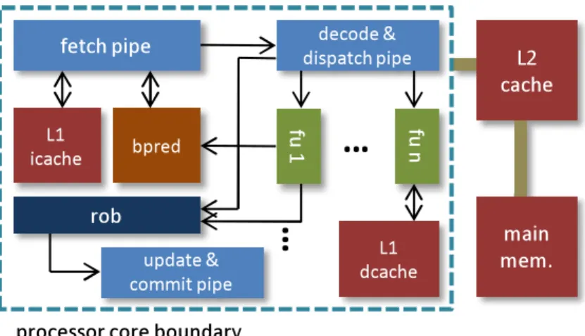
In this dissertation, a machine model is assumed to be a superscalar processor system with two levels of cache memory, L1 cache and L2 cache, and a main memory, as shown in Figure3. Program instructions and data are separately stored in L1 instruction cache and L1 data cache, respectively. The L2 cache is a unified cache which stores both the program instruc-tions and data. The superscalar processor core model used in this dissertation is sketched inside the dotted box. It has a front-end “fetch pipeline” that fetches instructions from the instruction cache and buffers the instructions for further processing. When a miss occurs in the instruction cache, the L2 cache is accessed to fetch the instructions. If the instruction fetch request also misses in the L2 cache, the main memory is accessed. The instruction fetch bandwidth provides an upper bound on the throughput of all subsequent pipeline stages [67]. It is determined by the instruction cache, branch predictor, and the processor parameters such as the instruction fetch queue size. To achieve sustainable instruction fetch bandwidth, it is important to minimize the branch mispredictions, since modern superscalar processors speculatively execute instructions fetched from a predicted path to increase the instruction-level parallelism (ILP). If the processor mispredicts the path, the processor rolls back to its state that was before the mis-predicted branch, and then executes the instructions fetched from the correct path. Many branch prediction schemes [52, 66] and instruction caching techniques [14,16,65] have been developed in the past for high bandwidth instruction fetch-ing.
Once fetched, instructions are decoded and dispatched to various functional units such as an ALU, branch unit, or data memory access unit. They may be temporarily stored
fetch pipe decode & dispatch pipe L1 icache bpred rob fu 1 fu n L1 dcache
…
update & commit pipe…
processor core boundary
L2 cache
main mem.
Figure 3: Machine model having a superscalar processor core, L2 cache, and main memory.
in buffers (or reservation stations) associated with a specific functional unit until the unit becomes available or until its input operands arrive. Due to the limited number of functional units in a processor, resource conflicts may occur when more than one operations compete for the same functional unit in the same cycle. When an instruction is dispatched, an entry is allocated in the reorder buffer (ROB) so that the “update and commit pipe” can change the architectural state properly in program order as instructions are committed in the pres-ence of special events such as exceptions, branch mis-predictions, and cache misses. The instructions are committed in program order by forcing an instruction to commit only when it becomes the oldest instruction in the ROB (the head of the ROB). Only the instructions in the ROB without any unresolved dependencies are considered to be scheduled at any given time. Hence, the size of the ROB is an important parameter to achieve high instruction-level parallelism or memory-level parallelism. For instance, with a 96-entry ROB, two instruc-tions cannot be simultaneously executed if they are 96 or more instrucinstruc-tions away from each other [13,36]. ROB holds the result of an operation until the associated instruction commits, and provides the result to the depending instructions. For memory instructions, the memory dependency is examined in addition to the data dependency between instructions. When scheduling a load instruction, the store buffer is searched for a preceding store instruction with an unknown memory address. If there is such store instruction, the load instruction
cannot be issued until the memory address of the preceding store instruction is calculated. Because of the disparity between the processor and memory speed [77,79], the cache sub-system plays a critical role in achieving high performance, particularly for memory-intensive programs, by reducing the number of accesses to the main memory. It exploits the local-ity presented in a program and stores frequently accessed data to avoid accessing the main memory. The cache subsystem consists of multiple levels of hierarchy, where the upper level caches are faster and smaller than the lower level caches. Modern superscalar processors typically use two or more levels of caches. In this dissertation, the notion of “last-level cache (LLC)” is used to indicate the last level of cache on chip before accessing the off-chip main memory. The processor schedules a memory instruction to a load/store unit which issues a cache access to the L1 data cache. When the cache access misses in L1 data cache, it accesses the lower level caches until it hits in the cache or it reaches the LLC. If the access misses in LLC, it accesses the off-chip main memory. Since the target machine assumes a two-level cache hierarchy, L2 cache is the LLC in the target machine. The L2 cache may be placed in-side or outin-side (uncore) the processor core. The L2 cache that is placed inin-side the processor core is private to its processor core, whereas uncore L2 cache can be either private or shared among the processor cores. It is noted that the uncore shared L2 cache and main memory are considered as a system-wide resource in multicore processor architectures [23, 38].
To achieve high performance, it is important to reduce the amount of accesses to the main memory and hide the main memory access latency as much as possible due to the long main memory access latency. L2 cache data prefetching may reduce the number of L2 cache misses by speculatively loading the data that are likely to be used in a near future from the main memory to the L2 cache. In this dissertation, a sequential data prefetching technique, tagged prefetch [69], and a stream-based prefetching [71] are employed. The tagged prefetch algorithm uses a tag bit, which is used to mark prefetched blocks that are reused, associated with every cache block. Tagged prefetcher triggers a prefetch request for cache block B + 1, when a cache miss occurs on cache block B, or when a hit occurs on a prefetched cache block B. The stream prefetching algorithm, unlike the simple sequential data prefetching algorithms, monitors the cache access streams and triggers a prefetch request when the cache access is determined to be a part of an identified stream.
To hide the long main memory access latency, the cache subsystem supports multiple outstanding requests to the main memory to overlap the main memory accesses. If two independent main memory accesses occur simultaneously, only the latency of single main memory access will be exposed to the processor. Miss status handling registers (MSHRs) are used to hold the information of an outstanding cache miss until the cache miss is resolved. Hence, the number of outstanding L2 cache misses is determined by the number of L2 MSHRs in the system. An MSHR holds the primary miss and many secondary misses to a cache block. A primary miss is the first cache miss to a cache block and secondary misses are the following cache misses to the same cache block (i.e., delayed hits).
More general description of superscalar processor design and operation can be found in Hennessy and Patterson [31], Johnson [33], and Shen and Lipasti [67].
2.2 PERFORMANCE MODELING METHODS
Before the actual hardware of a target processor system is available, the performance of the target system is estimated using performance modeling techniques. The two most common performance modeling methods are (software) simulation and analytical modeling. It is well known that simulation is accurate than analytical modeling techniques, however, it suffers from long simulation time. On the other hand, analytical modeling techniques are less accurate than simulation, however, they have a clear speed advantage over simulation. Simulation can be classified into execution-driven simulation, which executes actual program instructions, and trace-driven simulation, which is driven from a stored trace file1. Table 1 compares three popular performance modeling methods: execution-driven simulation, trace-driven simulation, and analytical modeling.
An execution-driven simulator consists of a functional simulator and a timing simulator. The functional simulator implements an instruction set architecture that can execute a real 1Trace-driven simulation may directly use the trace without storing the trace in a disk using on-line tracing techniques. However, this dissertation assumes that trace-driven simulation uses stored traces. On-line method does not incur storage space overheads, however, it does not allow traces to be shared and makes it difficult to obtain repeatable simulation results [40].
Methods Speed Required disk space size
Execution-driven Application-only Slow —
simulation Full-system Very slow Small
Trace-driven Full-trace Slow Large
simulation Filtered-trace Fast Moderate
Analytical modeling Very fast May require large space
Table 1: Comparing different performance modeling methodologies.
binary. It decodes the instructions in program order to get their operands and store operation results in the target register. The timing simulator, also known as performance simulator, models the processor microarchitecture artifacts. It takes the machine configuration and the decoded instruction information as input and collects various statistics to measure the performance.
There are two types of driven simulation. One is an application-only execution-driven simulation, which simplifies the handling of I/O operations and operating system activities. When simulating a program binary on an application-only execution-driven sim-ulator, the system calls from the binary are emulated by calling the host operating sys-tem. Simplescalar [2] is a popular application-only execution-driven simulator suite used in academia. The simulator suite has a fast functional simulator and a detailed timing sim-ulator that models an out-of-order superscalar processor. The other type is a full-system execution-driven simulation, which models the complete hardware system in enough detail to run unmodified operating systems. There are many workloads that require an entire system simulation to obtain meaningful simulation results, such as the database and server work-loads [72] and multithreaded workwork-loads [7]. Examples of well-known full-system simulators are SIMICS [50], QEMU [6], gem5 [8], and MARSSx86 [63]. SIMICS and QEMU functionally simulates the entire computer systems, but do not provide modules for timing simulation of processor systems. Hence, SIMICS and QEMU users must develop their own modules to simulate a processor system. An example is GEMS [51], which is a set of modules for SIMICS that models the detailed microarchitecture of multiprocessor systems. On the other hand, gem5 and MARSSx86 simulators provide both the functional simulator and detailed
timing model to simulate a processor architecture. Unlike an application-only simulator, a full-system simulator requires few giga-bytes of storage space to keep an image of the disk.
Trace-driven simulation replaces the functional simulation of the execution-driven sim-ulation with pre-generated traces. Once the traces are generated, the traces can be reused many times for timing simulation. The traces may be a full instruction trace or traces of cer-tain events, such as memory references. Conventional trace-driven simulation for superscalar processors employs a full instruction trace to simulate the dynamic behavior of a superscalar processor [62]. However, a full instruction trace requires a large storage space. Moreover, trace-driven simulation with a full instruction trace does not have a clear speed advantage over an execution-driven simulation, since they both simulate the entire instruction stream of a program. On the other hand, filtered-trace simulation requires a much smaller storage space since it only traces specific events rather than the entire instructions of a program. For instance, Dinero IV [11] is a cache simulator that takes memory reference traces and provides the cache hit and miss information. This dissertation focuses on filtered traces that capture only a subset of memory references.
Analytical modeling relies on mathematical equations to model the superscalar processor performance based on several simplifications. It can provide valuable insights in the early processor design stages, and it has a speed advantage over other simulation methods [36]. However, it only provides the estimated performance numbers as the end result, and it cannot reproduce the dynamic behavior a superscalar processor. For accurate performance modeling, analytical models require an instruction trace analysis for each program to obtain the necessary information for their mathematical models.
During processor development, computer architects select appropriate performance mod-eling methods depending on the purpose and requirement of the modmod-eling work. For instance, to obtain highly accurate simulation results, a detailed cycle accurate execution-driven simu-lation is used. On the other hand, if the focus of a study is limited to certain events, filtered trace-driven simulation can be used for faster simulation speed. For example, in this dis-sertation, the processor core is abstracted and filtered trace-driven simulation is used, since the focus of the work is on assessing the impact of uncore accesses on superscalar processor performance.
2.2.1 Trace-driven simulation
Trace-driven simulation is a widely practiced simulation method due to its fast simulation speed and reduced programming effort compared to other detailed simulation methods, such as execution-driven simulation. Trace-driven simulation consists of two phases [73, 82]. In the trace generation phase, a benchmark is executed and information about key events is recorded in a trace file. In the trace simulation phase, the information recorded in the first phase is used to drive the simulation. The history of trace-driven simulation goes back several decades [69, 73]. In 1966, Belady used trace-driven simulation method to study the replacement algorithms for a virtual storage computer [5].
Trace-driven simulation’s increased speed is a result of replacing the detailed functional execution of a benchmark with a pre-captured, but highly representative, trace of an exe-cution. However, accuracy issues arise when using trace-driven simulation for superscalar processors and multicore processors. Black et al. [10] questioned the accuracy of trace-driven simulation for superscalar processors even when the full traces were used as the processor complexity continues to increase and the benchmarks evolve to run for longer times. They also determined that sampling techniques present a problem to the accuracy of trace-driven simulation for superscalar processors. Bitar [9] and Goldschmidt and Hennessy [30] discussed the accuracy of trace-driven simulation for multiprocessor studies. Parallel workloads run-ning on a multiprocessor system are likely to introduce timing-dependencies in the memory traces due to the asynchronous interactions between processes (threads), such as dynamic al-location of shared resources and barrier synchronization. The timing-dependencies in trace incur large inaccuracies when trace-driven simulation is used for multiprocessor systems. Nevertheless, Goldschmidt and Hennessy [30] introduced a technique for accurate trace-driven simulation of multiprocessors when timing dependencies are created by locks and barriers.
In previous and current practice, much trace-driven simulation work on memory system simulation has focused on either tracing memory references without timing [73] or using a full trace of executed instructions for relatively fast simulation with complete fidelity [4]. In the meantime, reducing traces has been considered important for practical reasons of storage
space and simulation speed. For instance, Chame and Dubois [12] used the property of cache inclusion to filter memory references that are guaranteed to hit in actual simulation and Iyengar et al. [32] defined an “R metric” to guide reducing trace sizes while still maintaining the branch related properties of the original traces. Wang and Baer [74] used a direct-mapped “filter cache” to filter memory references. Further work by Kaplan et al. [35] has yielded trace reduction techniques Safely Allowed Drop (SAD) and Optimal LRU Reduction (OLR), which accurately simulate the LRU policy. These further filter out hits, and OLR is provably optimal for the LRU policy. Agarwal and Huffman [1] proposed techniques to compress traces by exploiting spatial locality. Filtered tracing differs from sampling [68,80,81], since filtered trace items are generated throughout the execution of the program. However, previous trace-driven simulation works that use filtered traces have not been done in the context of timing accuracy for modeling superscalar processor performance.
In my previous work [45], I demonstrated that filtered trace-driven simulation can accu-rately approximate superscalar processor performance. In [45], I introduced three different trace-driven simulation models to approximate the impact of a long-latency memory access on superscalar processor performance with filtered traces: isolated cache miss model, indepen-dent cache miss model, and pairwise dependent cache miss model. However, the simulation models require a cycle-accurate execution-driven simulator that models the microarchitecture of the target superscalar processor to generate filtered traces.
In [44], I focused on the pairwise dependent cache miss model (PDCM) among the three strategies introduced in [45]. I presented the trace simulation algorithm in complete detail and discussed the improvements over [45] and many implementation issues. Moreover, I considered important architectural artifacts including: MSHR, data prefetching, and branch predictor. In [43], I proposed an abstract simulation method called In-N-Out to remove such limitation by using a functional cache simulator to generate filtered traces. Since a functional simulator does not provide timing information, In-N-Out resorts to information about data dependency between instructions to estimate the distance between L1 data cache misses.
Filtered trace simulation has been used for experiments with multithreaded parallel ap-plications. Eggers et al. [20, 21] use the memory references of parallel programs to analyze the sharing behavior of parallel applications to evaluate the performance of coherency
pro-tocols. In particularly, they analyze the memory reference patterns of write shared data in parallel applications. There are trace-driven multicore simulators that use filtered traces like this dissertation. Zauber [46] and TPTS [42] increase the simulation speed by replacing the core-level simulation with filtered traces. TPTS assumes in-order processor cores and does not model out-of-order superscalar processors. Zauber models out-of-order superscalar pro-cessors, however, their work lacked the details of the simulation methodology and evaluation of Zauber. Zauber uses Turandot [55] and TPTS uses Simplescalar and Simics [50] for col-lecting traces. PDCM and In-N-Out are expected to be easily integrated in such trace-driven multicore simulators.
Finally, traces for single-threaded or multi-threaded programs can be generated using inline tracing technique [21], rather than employing existing simulators. The technique automatically modifies the application binary to insert traps (codes) to collect traces dur-ing program execution. Similarly, binary instrumentation tools, such as PIN [49] and Val-grind [57], can be used to quickly generate instruction traces or filtered traces. There are also compiler-based tracing techniques [40] that can reduce the trace generation time and space overhead.
2.2.2 Analytical models for out-of-order superscalar processors
Due to its complexity, evaluating a modern superscalar processor’s performance with de-tailed simulation requires a great deal of efforts on implementing and validating a simulator. This motivated many researchers to develop alternative methods to quickly estimate the performance of a superscalar processor. Hence, much superscalar processor modeling work has focused on building an analytical model. There are four proposals [13, 24, 36, 52] the most related to this dissertation. They all used a functional simulator to generate instruc-tion traces prior to the actual modeling. The collected instrucinstruc-tion traces are then profiled to derive the parameters used in their analytical model.
Michaud et al. [52] built an analytical model to study the relations between instruction fetching, branch prediction accuracy, and ILP. In their model, they partitioned the full instruction trace into windows of constant size. They examined the length of the instruction
dependency chains in each window, and observed that the length of the longest instruction dependency chain can be used to estimate how many instructions can retire per cycle (IPC) and thereby derive the execution time.
Karkhanis and Smith [36] have presented a first-order analytical model for modeling a superscalar processor performance. Their first-order analytical performance model focuses on “miss events” that can stall program execution, such as branch misprediction, instruction cache miss, and data cache miss. Different equations are introduced to model individual penalties. The overall performance of a program is estimated with the baseline CPI (mea-sured with no miss-events) and the CPI due to these miss events.
Chen and Aamodt [13] extended the first-order model [36] by more accurately estimating the CPI component due to long latency data cache misses. They proposed a method to analytically model the effect of pending data cache hits, data prefetching, and MSHRs, which were not considered in the first-order model. They also demonstrated that their model can estimate the individual effect of data prefetching and MSHRs, and their combined effects as well. Their model considered the effect of pending data cache hits, which was not considered by Karkhanis and Smith. This dissertation also discusses the importance of considering the pending data cache hits and modeling their effect accordingly. Chen and Aamodt assumed perfect branch prediction and instruction caching.
Eyerman et al. [24] proposed a “mechanistic model” which is a revision of the first-order model. They model the execution time between two miss events, namely “interval”, and the overall execution time is derived by simply aggregating the execution times of all intervals. For simpler performance penalty formulation, their model focused on the dispatch stage of the processor, whereas the first-order model focused on the instruction issue stage. Similar to Karkhanis and Smith, they modeled branch prediction and instruction caching, but did not model the effect of pending data cache hits, data prefetching, and MSHRs. More recently, Genbrugge et al. [29] proposed “interval simulation”, which extends the mechanistic model [24] to raise the level of abstraction for fast multicore simulation. They use a functional simulator to generate a dynamic instruction stream for their model. The significant difference between simulation methods and these analytical models comes from the usage of these models. The goal of using an analytical model is to quickly derive the overall performance
Techniques Technique description
Sampling Find the representative simulation points of a program
Workload characterization Develop an alternative program to replace a large program
Increasing the abstraction
level
Focus on a few aspects that are most critical to the performance
Parallel simulation Achieve simulation speedup by parallelizing a single simulation
Table 2: Various techniques to reduce the simulation time.
number as an end result using mathematical equations, whereas a simulation method is used as a tool to estimate the performance and observe the behavior of a target system.
Noonburg and Shen [58] have proposed a framework for statistical modeling of super-scalar processors. Eeckhout et al. [19] compares different simulation methods and advo-cates the advantage of using statistical simulation than other simulation methods, such as trace-driven and execution-driven simulation, when detailed performance modeling is not necessary. Nussbaum et al. [59,60] also proposed using statistical simulation for superscalar processors and symmetric multiprocessor system.
While a model-based approach is extremely useful when considering a few design param-eters quickly, it does not diminish the role of fast and accurate simulation methods like the ones developed in this research. The significant difference between the simulation methods presented in this dissertation and these analytical models comes from the usage of these models.
2.2.3 Other simulation time reduction techniques
While not directly comparable to the dissertation, there are other techniques to reduce the simulation time, as listed in Table 2. Sampling techniques have been developed to reduce the scope of (detailed) simulation during execution-driven simulation. Sherwood et al. [68] proposed SimPoint, a technique to automatically identify “representative” program intervals that exhibit stable behavior (called “phases”). One could choose to simulate portions of these intervals (e.g., 100M instructions) to predict a benchmark’s execution time and other metrics
rather than simulate the whole execution, thereby effectively reducing the time needed for simulation. According to [68], each SPEC2k benchmark program has up to 10 phases. Considering that typical SPEC2k benchmarks execute hundreds of billions of instructions, SimPoint has the potential to reduce the amount of detailed simulation by a factor of ∼100 (100M per phase x 10 phases / 100B instructions). The average IPC error of SimPoint based simulation, compared with sim-outorder, was reported to be ∼3% over the SPEC2k benchmarks.
Another sampling method, SMARTS, was proposed by Wunderlich et al. [80]. Unlike SimPoint that reduces the scope of detailed simulation to specific phases, SMARTS system-atically samples program execution intervals with relatively fine granularity without paying attention to program behavior changes. The number of samples and the length of each sam-ple depend on the desired target confidence level. Compared with sim-outorder, SMARTS was shown to achieve 60× simulation speedup and less than 1% error (on average). Com-pared with SimPoint and SMARTS, the techniques presented in the dissertation resort to cache filtering, a fundamentally different sampling strategy with no bearing on simulation intervals. The proposed methods offer an orthogonal method to speed up detailed simula-tion itself by focusing on a subset of processor events (cache misses) and abstracting away other details. Naturally, they could work together with either SimPoint or SMARTS (in the context of trace-driven simulation).
Ekman and Stenstr¨om [22] used statistical method “matched-pari” comparison to mini-mize the number of simulation points of a program to achieve certain accuracy. Wenisch et al. [75] presented a sampling framework that replaces “functional warming” with live-points without sacrificing accuracy. Functional warming warms up large microarchitecture building blocks, such as caches and branch predictor, while running functional simulation to quickly move to the next simulation point [80].
Workload characterization is used to develop an alternative program that can replace the long-running benchmark program. One such example is synthetic workloads. Synthetic workloads are not a user program, but they capture the characteristics of the real bench-marks that they wish to represent. Ganesan et al. [27] developed a framework that gener-ates synthetic clones for the target benchmarks using the characterized information of the
benchmarks. Genbrugge and Eeckhout [28] improved the statistical simulation methodology by using synthetic trace and an accurate memory data flow model, which models delayed hits, RAW (read after write) memory dependencies, and cache miss correlation. On the other hand, MinneSPEC tries to reflect the behavior of SPEC2K benchmarks while using a smaller, but representative input set [37]. Using this workload, simulation results can be obtained in a reasonable time without developing new simulation techniques. The simulation time is expected to be further reduced, if filtered traces generated with synthetic workloads or MinneSPEC are used in the simulation methods proposed in this dissertation.
There are simple yet effective performance modeling works that achieve fast and accu-rate performance estimation by increasing the abstraction level. An example is profile-based approaches. Profiled-based performance estimation techniques run in two phases, mentation and analysis, similar to that of the trace-driven simulation method. In the instru-mentation phase, the instruinstru-mentation tool instruments a benchmark to count the number of times each basic block is executed in a specific run. In the analysis phase, the execution time of each basic block in a program are estimated using a simple pipeline simulator. The program execution time is then estimated as T =∑numBBsi=0 Ti×Counti, wherenumBBsis the number of static basic blocks in a program, Ti is the time spent to execute basic block
i, and Counti is the number of times basic blocki was executed in a specific run [61]. Such approach works well for a simple in-order processor. However, very large errors are shown when the above approach is applied for superscalar processor because it does not consider the key characteristics of a superscalar processor, such as out-of-order issue, long dependency arcs that cross basic block boundaries, etc. The reported error compared with a trace-driven simulator was 125% on average using SPEC95 benchmarks [70]. The large average error can be reduced to 43.4% by using a path tracing technique [3]. Ofelt and Hennessy [61] fur-ther reduced the average error of using profile-based performance prediction for superscalar processors to 1.25% by using their “Pairwise Analysis Algorithm (PAA)”.
Loh [48] introduced a time-stamping algorithm to model superscalar processor perfor-mance using a functional simulator. The time-stamping algorithm concentrates on the time when a particular event can occur rather than simulating the processor cycle by cycle. Fields et al. [25, 26] proposed a method to construct a critical path of a program for
microarchi-tectural performance analysis. The critical path is defined as a sequence of instructions in a program that has the longest cumulative latency. Their work is based on the assumption that the performance of a superscalar processor is mainly determined by the events on the critical path. Chou et al. [15] introduced a simulation method based on their epoch model to quickly derive the memory-level parallelism (MLP) of a program. Their simulator, MLPsim, is a very simplified processor model based on several assumptions. Nonetheless, the simulator shows accurate MLP results, especially when a long off-chip access latency is assumed.
Architects run many simulations in parallel to reduce the overall simulation time. Wenisch et al. [76] proposed a simulation framework that can be parallelized using their checkpoints. Since each checkpoint [75] can be simulated independently, users can run hundreds of simu-lations in parallel using hundreds of checkpoints on many host machines. Similarly, a single simulation may be parallelized to reduce the simulation time. Mukherjee et al. [56] presented a tool called wisconsin wind tunnel (WWT) II that enables a parallel, discrete-event, direct-execution simulation. In their work, they identified four key operations that can underlie parallel, discrete-event, direct-execution simulation and made alternative implementations of the four key operations in their tool. Assuming a 32-node target machine, WWT II achieves a speedup of 4.1−5.4 when using 8 host processors. More recently, Miller et al. [53] introduced a distributed parallel multicore simulator infrastructure named Graphite. Using their framework individual simulation is distributed across a cluster of servers to accelerate simulation, which works in a completely transparent fashion to the applications. Graphite achieves near linear speedup on a simulation of a 1000-tile target using from 1 to 10 host machines. Finally, Moeng et al. [54] proposed using Graphics Processing Units (GPUs) to accelerate manycore architectural simulation. They showed that using GPUs for parallel simulation can achieve better scaling with core count then other techniques by implementing a trace-driven many cache simulator using NVIDIA’s CUDA toolkit.
3.0 TRACE SIMULATION WITH TIMING INFORMATION
3.1 OVERVIEW
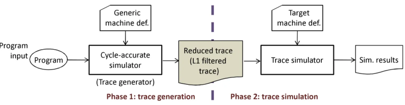
In this chapter, three trace-driven simulation models that use timing-aware traces are intro-duced. Unlike most previous work that uses a trace-driven simulation framework [73], the notion of timing is introduced during the trace generation phase and embed time-related information in the trace. Hence, the trace generator must be able to model the microar-chitecture of a processor using a user provided machine definition. Figure 4 illustrates the relationship between the trace generator, trace simulator, machine definitions, and trace files. The generic machine definition refers to the superscalar processor core configuration: the intra-core parameters that shape the processor core described in Section 2.1. The target machine definitionis the system-level processor configuration such as L2 cache configuration and main memory access latency, that completes the overall machine model. Throughout this dissertation, sim-outorder, a detailed out-of-order processor simulator of the SimpleScalar tool set [2], is used to generate traces.
The proposed models use timing-aware filtered traces. That is, trace files do not contain all executed instructions during program execution and rather focus on memory access in-structions [73]. Moreover, L1 cache hits that do not access the L2 cache are filtered out, further cutting down the number of trace items to store in trace files, similar to [12, 42, 46]. Each trace item in the timing-aware filtered traces captures: (1) the number of executed in-structions after the last trace item, (2) the number of elapsed cycles since the last trace item, and (3) the information of the memory instruction that generated the trace item (L1 cache miss): cache access type (data read, data write, or instruction fetch), instruction sequence number, cache address, and write-back address (if a write-back occurred on a cache miss).
Target machine def.
Program Program
input Cycle-accurate Sim. results
simulator Trace simulator
Generic machine def.
Reduced trace (L1 filtered
trace)
Phase 1: trace generation Phase 2: trace simulation
(Trace generator)
Figure 4: Overall structure of PDCM. It uses a cycle-accurate simulator to generate reduced traces (L1 filtered traces).
In this section, three trace-driven simulation methods are presented and evaluated to quantify the impact of a long-latency memory access in a superscalar processor with timing-aware filtered traces. The strategies are based on three different models about how a cache miss is treated with respect to other cache misses: (1) isolated cache miss model, (2) inde-pendent cache miss model, and (3) pairwise deinde-pendent cache miss model. It is important to note that, in the proposed methods, the processor core configuration used in the trace generator must be identical to the core configuration of the simulated machine. This work assumes that the processor core parameters, such as branch prediction algorithm, ROB size, available functional unit types, and L1 cache configuration, are fixed when the focus of study is on the “uncore” components of a processor chip.
3.2 MODEL 1: ISOLATED CACHE MISS MODEL
3.2.1 Basic idea
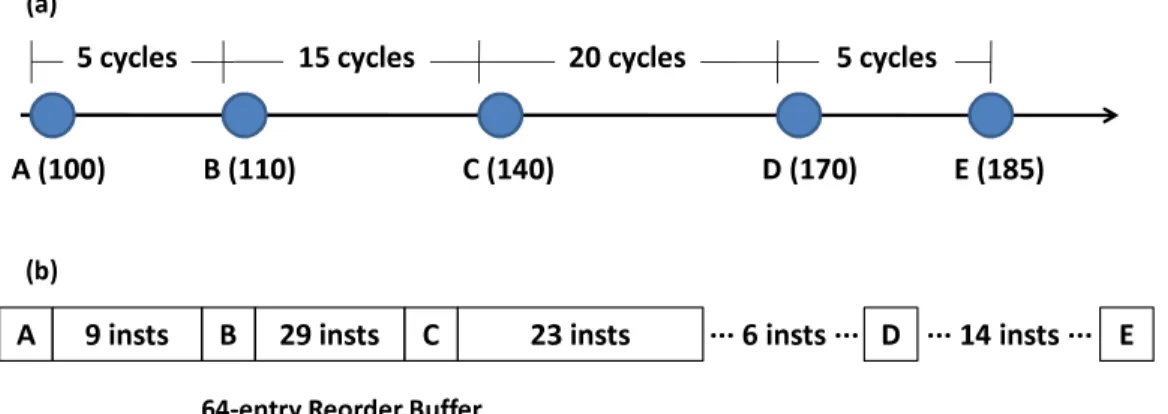
The basic idea of this model is quite simple: The actual impact of a particular cache miss on the overall program execution time is the time difference of two program runs, one without the miss and one with the miss, assuming that all other memory access latencies are unchanged. Figure5(a) captures this idea. Program run 1 has no L2 cache misses, whereas program run
run 1
run 2
L1 miss, L2 hit L1 miss, L2 miss
(a) run 1 run 2 (b) run 3 interval (n+1) interval (n) trace item (n+1) trace item (n)
…
…
…
…
…
…
Figure 5: (a) A single “isolated” L2 cache miss in a program run. (b) Using two additional traces generated by interleaving hits and misses to efficiently compute the impact of isolated misses on program execution time.
2 of the same program has a single L2 cache miss at a known L2 cache access. The impact of the cache miss on the execution time of the program is simply (Trun 2−Trun 1). Trun 1
can be obtained using a cycle-accurate simulator modeling a perfect L2 cache having a 100% hit rate. Trun 2 can be obtained by using the same cycle-accurate simulator and giving the
L2 cache miss penalty to a specific L2 cache access. One can measure the impact of each and every potential L2 cache miss by repeating this process.
3.2.2 Instruction permeability analysis
While the basic idea of the isolated cache miss model is intuitive, the process of assessing the impact of each potential L2 cache miss can be extremely time consuming. Suppose that a program has N L1 cache misses. In an exhaustive approach to analyze this program, for instance, one will generate N traces (each having exactly one L2 cache miss) and compare them against the trace having no L2 cache misses to deduce the impact of each individual cache miss.
L2 cache miss, a technique calledinstruction permeability analysis is used to systematically assign a cache access latency to trace items as they are generated in the trace generation phase. Figure 5(b) shows three traces generated from a target program for instruction permeability analysis. One trace has only L2 cache hits and the other two have alternating L2 cache hits and misses. The alternation of cache hits and misses is skewed in the two traces so that all trace items are covered. By comparing the actual number of cycles measured in trace intervals, each surrounded by two trace items, the impact of a single L2 cache miss can be computed as would have been done with a trace having only a single L2 cache miss. The configuration sketched in Figure 5(b) is called 2-interleaving because the additional traces have one L2 cache miss every two trace items.
In what follows, we discuss how the impact of a cache miss is analyzed and how such information is associated with trace items. Assume that S is the latency of a cache hit and
L is the latency of a cache miss. L is the latency penalty paid on a specific cache miss (i.e., main memory access) on top of a cache access latencyS. From measurements one can obtain
a, the cycle count of the interval (n) after trace item (n) in trace 1 and b, the cycle count of the same interval in trace 2. dn is defined as b−a. Because the nth trace item in trace 2 has a longer latency (S+L) than the latency of the corresponding trace item in trace 1 (S), b > a holds and equivalently dn >0. Once dn is obtained, trace item (n) is annotated with the timing information (a,∆n) where ∆n is defined as (L−dn). Given this, the actual latency of interval (n) during the trace-driven simulation is:
a if trace item n hits in L2 cache and
a+L′−∆n if trace item n misses in L2 cache
where L′ is the actual main memory access latency used in the trace-driven simulation. When L = L′, the method guarantees that the actual latency computed for interval (n) is
a or b depending on the cache access outcome of trace item (n), the same as those of the timing-aware trace generation. If L̸=L′, the actual latency will be either aor (b+η) where
η=L′−L.
The above description of instruction permeability analysis used a 2-interleaving configu-ration. One may choose to employ a 3-interleaving configuration where there is one L2 cache
Dispatch/issue/commit width 4
Reorder buffer (ROB) 64 entries
Integer /Floating point ALUs 4/2
L1 i- & d-cache 1 cycle, 16KB, 4-way, 64B line size, LRU
L2 cache (unified) 12 cycles, 1MB, 8-way, 64B line size, LRU
Branch prediction Perfect
Main memory latency 300 cycles
Table 3: The baseline machine configuration for evaluating the isolated cache miss model.
miss every three trace items. Obviously the most important factor affecting the effectiveness of this scheme is how far in time trace items are separated from each other. If a “missed” trace item is far away from the next missed trace item in trace 2 and 3 in the example of Figure 5(b), the result of the analysis will be a close approximation of what would have been obtained from the exhaustive method. Hence, it is expected that an n-interleaving configuration will result in higher accuracy than an m-interleaving configuration if n > m, at a higher trace generation and analysis cost. If n = N where N is the number of trace items, the n-interleaving configuration degenerates to the exhaustive method.
3.2.3 Experimental setup
Table 3shows the baseline machine configuration that is used to evaluate the isolated cache miss model and the independent cache miss model (in Section3.3). An ideal instruction cache and a perfect branch predictor are used to isolate the interferences caused by instruction cache misses and branch mispredictions. To evaluate the isolated cache miss model and the independent cache miss model, a selected set of SPEC2K benchmarks is used: mcf, art (benchmarks with high L1 cache miss rates),gcc,ammp(with medium L1 cache miss rates),
perl and facerec (with low L1 cache miss rates). Selection was based on their L1 cache
miss rates and the raw instruction level parallelism (ILP) present in the programs, such that strengths and weaknesses of the studied strategies can be exposed. The entire benchmarks in the SPEC2K benchmark suite are used to evaluate the pairwise dependent cache miss model (in Section3.4) and In-N-Out (in Section4). The inputs for the entire SPEC2K benchmarks
Integer Input Floating point Input
mcf inp.in art c756hel.in
gzip input.graphic galgel galgel.in
vpr route equake inp.in
twolf ref swim swim.in
gcc 166.i ammp ammp.in
crafty crafty.in applu applu.in
parser ref lucas lucas2.in
bzip2 input.graphic mgrid mgrid.in
perlbmk diffmail apsi apsi.in
vortex lendian1.raw fma3d fma3d.in
gap ref.in facerec ref.in
eon rushmeier wupwise wupwise.in
mesa mesa.in
sixtra