econ
stor
www.econstor.eu
Der Open-Access-Publikationsserver der ZBW – Leibniz-Informationszentrum Wirtschaft
The Open Access Publication Server of the ZBW – Leibniz Information Centre for Economics
Nutzungsbedingungen:
Die ZBW räumt Ihnen als Nutzerin/Nutzer das unentgeltliche, räumlich unbeschränkte und zeitlich auf die Dauer des Schutzrechts beschränkte einfache Recht ein, das ausgewählte Werk im Rahmen der unter
→ http://www.econstor.eu/dspace/Nutzungsbedingungen nachzulesenden vollständigen Nutzungsbedingungen zu vervielfältigen, mit denen die Nutzerin/der Nutzer sich durch die erste Nutzung einverstanden erklärt.
Terms of use:
The ZBW grants you, the user, the non-exclusive right to use the selected work free of charge, territorially unrestricted and within the time limit of the term of the property rights according to the terms specified at
→ http://www.econstor.eu/dspace/Nutzungsbedingungen By the first use of the selected work the user agrees and declares to comply with these terms of use.
Harttgen, Kenneth; Klasen, Stephan; Misselhorn, Mark
Conference Paper
Education for All? Measuring Pro-Poor
Educational Outcomes in Developing
Countries
Proceedings of the German Development Economics Conference, Zürich 2008, No. 22 Provided in cooperation with:
Verein für Socialpolitik
Suggested citation: Harttgen, Kenneth; Klasen, Stephan; Misselhorn, Mark (2008) : Education for All? Measuring Pro-Poor Educational Outcomes in Developing Countries, Proceedings of the German Development Economics Conference, Zürich 2008, No. 22, http:// hdl.handle.net/10419/39886
Education for All?
Measuring Pro-Poor Educational Outcomes in Developing
Countries
Kenneth Harttgen, Stephan Klasen and Mark Misselhorn∗ May 21, 2008
Preliminary Draft: Please do not cite.
Abstract
Achieving progress in education is of fundamental importance for hu-man development. Low levels of access to the education system and in educational outcomes in developing countries are often accompanied by high inequality between countries and within countries between popula-tion subgroups. This paper analyzes differences in improvements in the access to the education system and in educational outcomes across the welfare distribution between and within countries, and also by gender and regions for a sample of 37 developing countries using Demographic and Health Surveys (DHS). For the analysis, the toolbox of the growth incidence curves is applied to several educational indicators. We found an overall positive development in education. However, we do not iden-tify a clear pro-poor trend in progress in education between and within countries. We do find strong differences in education between males and females and between rural and urban areas. While gender inequality tends to decrease slightly, large differences by region tend to persist over time.
Key words: Pro-Poor Growth, Education, Growth Incidence Curve
∗University of Göttingen, Department of Economics, Platz der Göttinger Sieben 3, 37073
Göttingen, Germany, email: [email protected]. We would like to thank Elena Groß from the University of Göttingen. Any errors remain the responsibility of the author.
1
Introduction
At the beginning of the new century, shortcomings in education persist in many regions of the developing world, hampering economic growth and human de-velopment. Moreover, low levels of access to the education system and in edu-cational outcomes are often accompanied by high levels of inequality between countries, and within countries between population subgroups. Therefore, the success in addressing the challenge of progress in education requires national and multinational response.
In 1990, the World Conference on Education for All adopted the World Declaration on Education for All, which stated that everyone has a right to education. Because of insufficient progress in access to education and educa-tional outcomes in the developing world, in Dakar in the year 2000, the World Education Forum adopted a new framework for Action containing six Educa-tion for All (EFA) goals to be reached until the year 2015 to overcome the persisting shortcomings in education.1 In addition, two of the eight
Millen-nium Development Goals (MDG) committed by the United Nations (UN) in the year 2000 (in particular MDG 2 - achieve universal primary education - and MDG 3 - promote gender equality and empower women) directly emphasize the importance of education for human development.2 The explicit inclusion
of education among the MDGs reflects that these indicators are fundamental dimensions of human well-being.
Achieving progress in education is of fundamental importance for human development. A large body of literature shows that education accelerates eco-nomic growth, national productivity, political stability, and social cohesion (see, e.g. Chabott and Ramirez, 2000; Le Vine et al., 2004; Milligan et al., 2003). Education also has a direct impact on other dimensions of human
well-1
The six EFA goals adopted in the years 2000 to be reached until the years 2015 are: the expansion of early childhood care and education, the achievement of universal primary education, the development of learning opportunities for youth and adults, the spread of literacy, the achievement of gender parity and gender equality in education and improvements in education quality.
2
In particular, goal 1 is to eradicate extreme poverty and hunger, goal 2 is to achieve universal primary education, goal 3 is to promote gender equality and empower women, goal 4 is to reduce child mortality, goal 5 is to improve maternal health, goal 6 is to combat HIV/AIDS, malaria and other diseases, goal 7 is to ensure environmental sustainability and goal 8 is to develop a global partnership for development. Each of the eight goals breaks down to 18 quantifiable targets (UN, 2005).
being (i.e. the other MDGs) such as child health and nutrition (see, e.g. Duflo and Breierova, 2000 and Schultz, 2002). In addition, there also exists a strong relationship between education, poverty and inequality. On the one hand, edu-cation reduces poverty and inequality. Sustained economic growth and poverty reduction result in higher levels of household resources allowing higher invest-ments in their children’s education because parents are less dependent on their children’s labor. On the other hand, existing poverty and inequality may be worsened through poor education. Many researchers have shown that poverty significantly reduces the likelihood of school participation (see, e.g. Smith et al., 2007).
Today, more than half of the time period to reach the EFA goals and the MDGs has passed. During the last decade, many regions, particular in East and South Asia, have made significant progress towards the achievement of the goals by 2015 and many households and individuals have raised their levels of education. The latest EFA Global Monitoring Report provides a comprehensive mid-term overview of progress towards the Education for all goals set at Dakar in 2000. It shows that the world has made significant progress towards EFA since Dakar. For example, in developing countries, the net attendance rate in primary education has increased from 79 percent in 1991 to 86 percent in 2005. And concerning differences between the pre- and post-Dakar period, significant differences can be observed in the pace of progress. Faster progress has been made between 1999 and 2005 than between 1991 and 1999. For example, participation in primary education increased in Sub-Saharan Africa from 54 percent in 1991 to 57 percent in 1999 and 70 percent in 2005 (UNESCO 2008).
However, some regions and countries have lagged behind and some EFA goals or some aspects of them have been neglected. The regions that lag es-pecially behind the goals are the Arab states, Sub-Saharan Africa, West and South Asia (UNESCO 2008). Although Sub-Sahara Africa has been made sig-nificant progress over the last years, it still lags behind other developing regions (UN, 2007, UNESCO, 2007). In addition, whereas countries in South Asia and Latin America have made a lot of progress towards the goal of reducing the share of people suffering from hunger, many other regions and countries remain
well short of the targets, particularly in Sub-Saharan Africa, where many coun-tries are still stuck in a poverty trap. And besides improvements towards the the goal of universal primary education, there are still large shortcomings in many countries and a slow progress in primary completion rates remain a great concern in many regions. The same holds for adult education.
Furthermore, the progress towards the goals has also been uneven within countries. Wide disparities in progress remain between population subgroups, e.g. between males and females and rich and poor. There also exist significant within country differences in access to education and in educational outcomes especially between urban and rural areas (see, e.g. Lopez et al., 2007). For example, the 2008 EFA Report also indicates that progress in access to and participation in education has not benefited all children within countries and has led, in some cases, to greater sub-national disparities. Indeed, deeply entrenched disparities in opportunities for education based on income, gender, locality and other markers for disadvantage continue to represent a powerful obstacle to the realization of EFA. Hence, the question of the distribution and convergence in access and level of education of welfare sub-groups between countries and within countries, and in particular the question, of how progress in education is distributed across the population, is central to achieve the EFA goals.
In recent years, a fast growing field of literature in developing economics emerged that is concerned with the question of ‘pro poor growth’, i.e. how economic growth is distributed over the population. In particular, the question is whether the poor benefit from economic growth and social progress and if yes, to what extent (see e.g. Klasen, 2004 and Grosse et al. 2008), which is of particular policy relevance for achieving EFA goals and for reaching the MDGs.
The aim of the paper is to identify and understand, which parts of the population have benefited most or have not benefited from the improvements in the access to the education system and educational outcomes and to high-light the differences in the progress, if any, between the pre- and post-Dakar periods.3 The question whether the poor can benefit from progress in access
3
to the education system and educational outcomes is of considerable impor-tance because growth in monetary indicators of well-being does not necessarily lead to improvements in education. The analysis will provide a synthesis of the distribution, and changes over-time, of attendance rates and educational attainment in developing countries by income and other background charac-teristics like gender and urban versus rural areas. In particular, the following research topics will be analyzed: Which regions and countries have made the most progress towards the EFA goals and which regions still lack behind? Have inequalities both across and within countries been reduced? How do trends ob-served since the Dakar declaration differ from those that are obob-served in the period from 1991 and 1999?
The rest of the paper is organized as follows. Chapter 2 provides a short introduction in the concept of pro-poor growth and how one can introduce this concept to analyze pro-poor educational outcomes. Chapter 3 describes the methodology of the analysis and describes the data used. Chapter 4 presents the results. Finally, Chapter 5 concludes.
2
Assessing Pro-Poor Educational Outcomes
2.1 Concept and Definition of Pro-Poor GrowthPro-poor growth is often defined as economic growth that benefits the poor (e.g. UN, 2000; OECD, 2001, 2006). However, what remains to be specified using this broad definition is, first, if economic growth benefits the poor and, second, if yes to what extent. For example, Klasen (2004) provides more explicit requirements that a definition of pro-poor growth needs to satisfy. The first requirement is that the measure differentiates between growth that benefits the poor and other forms of economic growth, and it has to answer the question by how much the poor benefited. The second requirement is that the poor have benefited disproportionately more than the non-poor. The third requirement is that the assessment is sensitive to the distribution of incomes among the poor. The fourth requirement is that the measure allows an overall judgement of economic growth and not focuses only on the gains of the poor.
of the EFA 2000 assessment that was presented in Dakar in 2000. As for the pre-Dakar period, it covers years circa 1999.
Besides this approach there exist several other attempts conceptualizing pro-poor growth.4
In this paper, we use two broad definitions of pro-poor growth, namely absolute and relative pro-poor growth (see also Klasen, 2008). Pro-poor growth in the weak absolute sense means that the growth rates are, on average, above 0 for the poor. Pro-poor growth in the relative sense means that the income growth rates of the poor are higher than the average growth rates, thus that relative inequality falls.
2.2 Multidimensionality of Pro-Poor Growth
The most glaring shortcoming of all attempts to define and measure pro-poor growth is that they rely exclusively on one single indicator, which is income. This means that they are only focussed on MDG1 but leave out the multidi-mensionality of poverty, which is taken into account in the other MDGs.
Income enables households and/or individuals to obtain functionings. This means, income serves to expand peoples’ choice sets (capabilities) (Sen, 1987, 1988) and is, therefore, an indirect measure of poverty. In contrast, certain non-income indicators measure the functionings of households and individuals directly. Measuring poverty only with income assumes that income growth is accompanied by non-income growth. However, the problem of focussing only on MDG1 is that an improving income situation of households need not automatically imply an improving non-income situation, thus, reaching the other MDGs is not automatically guaranteed (for example, as shown in Klasen (2000) or Grimm et al. (2002)). While non-income indicators have recently received more and more attention in the concept and measurement of poverty5
there exists only some attempts to apply the concept of pro-poor growth to non-income indicators, such as education.
Grosse et al. (2008) introduce non-income indicators in the pro-poor growth
4
For a detailed review on the different definitions and measures of pro-poor growth, see, for example, Son (2003). Other approaches to define pro-poor growth are provided, for example, by White and Anderson (2000), Ravallion and Datt (2002), Klasen (2004), Hanmer and Booth (2001).
5
Examples for recent studies examining the multidimensional casual relationship between economic growth and poverty reduction are Bourguignon and Chakravarty (2003), Mukherjee (2001) and Summer (2003). Also international organizations point to the importance of the direct outcomes of poverty reduction such as health and education (see e.g. World Bank, 2000; UN, 2000; UN, 2000a).
measurement by calculating the growth incidence curves for several non-income indicators, such as education, nutrition, and health outcomes and apply this approach to Bolivia. The authors found an overall pro-poor development of all non-income indicators in Bolivia between 1989 and 1998. However, comparing the pro poor outcomes of the non-income indicators with the pro-poorness of income, the authors show that there exist no perfect correlation between the income and non-income dimension of poverty.
3
Methodology
3.1 Distribution of Educational Outcomes
To separate the population into welfare groups (i.e. percentiles, vintiles and/or quintiles) and in order to assess the access to and output of education in a coun-try and over time, one typically uses information on income or expenditure. As we do not have information on income or expenditure in the DHS data sets that we relay on for all of our analysis, we consider an alternative approach to define the socio-economic status of a household, which we use as a proxy for income or expenditure. In particular, we use an asset-based approach in defining well-being proposed by Filmer and Pritchett (2001) and Sahn and Stifel (2001). Although income or expenditure data is preferable, Sahn and Stifel (2001) show that such an asset index is an accurate indicator of long-term well-being if neither income nor expenditure are available. The main idea of this approach is to construct an aggregated uni-dimensional index over the range of different dichotomous variables of household assets capturing housing durables and information on the housing quality that indicate the material status (welfare) of the household:
Ai= ˆγ1ai1+...+ ˆγnain (1)
where Ai is the asset index, the ain’s refer to the respective asset of the
household i recorded as dichotomous variables in the DHS data sets and the
ˆ
γ are the respective weights for teach asset that are to be estimated.
use a principal component analysis proposed by Filmer and Pritchett (2001).6
In particular, as the components for the asset index, we include dichotomous variables whether the following assets in a household exist or not: radio, TV, refrigerator, bike, motorized transport, capturing household durables and type of floor material, type of wall material, type of toilet, and type drinking water capturing the housing quality.
The use of the asset index approach to derive a welfare distribution faces some critical issues that should be mentioned when using this approach as a proxy for income. The asset index can be biased, because it might not reflect correctly differences in income between rural and urban areas, due to usually huge differences in prices and the supply of such assets as well as differences in preferences for assets between both areas. For example, urban households possess demand other assets than rural households. To deal with this issue, for the analysis of differences in access to education and in educational out-comes between rural and urban areas, therefore, we calculate the asset index separately for urban and rural areas.
After having derived the aggregated index, one can derife the welfare dis-tribution and classify population welfare subgroups p. For example, using quintiles as the segmentation dimension, quintile 1 would correspond to the poorest population subgroup and quintile 5 to richest, respectively. Using this welfare distribution, we analyze the access to the education system and edu-cational outcomes, measured by several indicators that are described below, by welfare groups within countries for several periods and also over time to show trends in progress towards the EFA goals and differences ion the progress made between the pre- and post-Dakar period.
3.2 The Non-Income Growth Incidence Curve
A often used tool for answering the question of whether and, if yes, to what extent growth was pro poor is the GIC (Ravallion and Chen, 2003), which shows the mean growth rategt in income y at each percentile p of the
distri-bution between two points in time,t–1 and t. The GIC links the growth rates
6
An alternative way to estimate the weights for the assets to derive the aggragted index is a factor analysis employed, for example, by Sahn and Stifel (2001). However, the two estimation methods show very similar results.
of different percentiles and is given by
GIC :gt(p) =
yt(p)
yt−1(p)
−1,∀p= 1,2, . . . ,100. (2) By comparing the two periods, the GIC plots the population percentiles (from 1–100 ranked by income) on the horizontal axis against the annual per capita growth rate in income of the respective centile. If the GIC is above 0 for all percentiles (gt(p) > 0 for all p), then it indicates absolute pro-poor growth.
If the GIC is negatively sloped it indicates relative pro-poor growth. It is important to note that we assume anonymity throughout, i.e. we consider the growth rates of percentiles, even though they contain different households or individuals in the two periods.7
To calculate the non-income growth incidence curves to measure the pro-poorness of improvements in education, we follow the approach of Grosse et al. (2008). The calculation of the non-income growth incidence curves (NIGIC) broadly follows the concept of the GIC. Instead of income (y), we apply Equa-tions (2) to selected education indicators to measure pro-poor progress in ed-ucation directly via outcome-based welfare indicators over time.
In general, the growth incidence curve for education indicators can be cal-culated in two different ways. The first way, we call conditional NIGIC in which the individuals are sorted by income and calculate based on this income ranking the population percentiles of the education variables. With the condi-tional NIGIC, one can adress the question whether and, if yes, to what extent the income poor population subgroup have benefited from improvements in education compared to the income richer population subgroups. In addition, on can capture the problem that the assignment of the households to income percentiles on the one hand (GIC) and to non-income percentiles on the other hand (unconditional NIGIC) might not be the same. For example, the income-poorest group might not be the education-income-poorest group at the same time. This means that, in the conditional NIGIC, the percentiles are income percentiles, thus that the ‘poorest’ percentile is the one with lowest income, but that the
7
One should be cautious when deducing policy implications from the GIC when assuming anonymity. In particular, the GIC allows not to show if, for example, specific policy measures were beneficial to those who where poor in the initial period, but can show if the poor in both periods have benefited more from the measures than the non-poor. For a discussion of this and results when the anonymity axiom is lifted, see Grimm (2007).
growth rates are non-income growth rates, thus, are calculated for, e.g. years of schooling of the income percentiles.
The second way is to rank the individuals by each respective education in-dicator and generate the population percentiles based on this ranking. Based on distribution one can than calculate growth rates for each respective educa-tional indicator along the educaeduca-tional distribution. In other words, one asks whether the education poor population have benefited more from improve-ments in education than the education richer population subgroups. This, we call the unconditional NIGIC. For example, using average years of schooling of adult household members, the ‘poorest’ percentile is now not the income-poorest percentile but the one with the lowest average household educational attainment.
Both ways of calculating the NIGIC are of particular relevance for policy making. The conditional NIGIC provides a tool to investigate how the progress in non-income dimensions of poverty was distributed over the income distri-bution. This mean that it allows to interplay between education and poverty. This is also of relevance when evaluating distributional impacts of aid and public spending. Standard benefit incidence studies, for example, analyze the impact of public spending by calculating shares of the total spending to each percentile and comparing the shares of the income poorest with the income richest centile (see e.g. Van de Walle, 1998; Van de Walle, 1995; Lanjouw and Ravallion, 1998; Roberts, 2003). But the share of public spending for the poor serves only as a proxy for a real welfare impact in terms of non-income achieve-ments. With the conditional NIGIC, it is than possible to analyze the actual improvements in the particular social indicator over the income distribution. For example, it provides an instrument to assess if public social spending pro-grams has reached the targeted income-poorest population groups and if the public resources are effective allocated and used. For example, Berthélemy (2005) shows that education policies in Sub-Saharan Africa are biased against the poor. On average, policies favor the non-poor because they are concen-trated on improvements in secondary and tertiary education and only little attention is paid to improvements in primary eduction completion, i.e. to the poor population. In this respect, the conditional NIGIC might be a useful
tool in the pro-poor spending analysis to understand who benefits from public spending and to what extent. The unconditional NIGIC mirrors the devel-opment of the social indicators that are relevant for human welfare. Thus, it can monitor how the non-income MDGs (especially MDGs 2-6) have developed over time for different points of the non-income distribution. In order to reach the MDGs, improvements will be particularly important for those at the lower end of the non-income achievements and the NIGIC allows such an assessment. Whereas the growth incidence curve is calculated based on percentiles (p = 1,2, . . . ,100), in this paper, we calculate the growth rates, both for the conditional and unconditional distribution, based on vintiles (p= 1,2, . . . ,20). The reason for using vintiles instead of percentiles is to get a higher number of observations for each group when individuals are ranked by income. For example, if a percentile contains only 50 individuals (ranked by income) and if we assign to these percentiles the respective mean years of education, then it is possible to obtain huge variations within each percentile, which results in very wide confidence intervals between the growth in the two periods, and we will not be able to make precise statements about the income gradient.
4
Data
For the analysis of the improvements in education along the welfare distri-bution of populations and over time in developing countries, we use national representative Demographic and Health Surveys (DHS) for several countries and years. Besides information about household socio-economic characteris-tics, health, nutrition and infrastructure, the DHS data sets include also sev-eral indicators on education both for children and adults. Table 1 provides an overview about the countries and periods for which we use the DHS data sets for the analysis. In sum, we analyze the distribution of access to the education system and educational outcomes for 37 developing countries covering regions in Latin America, Africa and South East Asia. For 24 countries, we have data sets for 3 periods. This allows not only to capture changes in the access to the education system and in educational outcomes over time, but also to examine and analyze differences in these changes between the pre- and post-Dakar pe-riods in the distribution of access and outcomes of education by welfare groups
as well as by the other background characteristics such as urban and rural areas and/or by gender. For 13 countries we still have two periods allowing to examine and analyze changes over time. Is sum, we analyze the access to education and educational outcomes using 98 DHS data sets.
For the access to the education system, we use two indicators, the net at-tendance rates for primary and secondary education based on the respective country specific age structures.8 The means that, for example, the net
atten-dance rate to primary education in Bangladesh is calculated by dividing all children in the age group of 6-11 years that are enrolled in school by the total number of children of this age. To analyze the progress towards the goals of universal primary education, the attendance status is the most obvious indi-cator to use since it is the most basic element of school participation.
The net attendance rate of primary and secondary education considers only those children as enrolled who are in the official country specific age range (e.g. 6-11 and 11-17). Children of other ages, even if their are enrolled, are not taken into account. As the net attendance rate covers only the children in the official age range that is associated with a given level of education, the net attendance rate is also an indicator of the functional capability of the educational system, because a high net attendance rate is only possible if the education system has the capacity to educate entire cohorts and allow them to make progress according to their age.
To assess the educational attainment in each country and across the welfare distribution within countries, we use two different indicators for two different age groups. First, we use average years of schooling completed and, second, the completion rates of primary, secondary or higher education. As the two age groups of adults, we use the age group aged between 17 and 22 and between 23 and 27. Age plays an important role when analyzing changes in non-income indicators, especially for education. In particular, not much improvements in education can be expected among the adult population (for example the education of 30-40 year olds in the first period should not be be very different from the education of the 40-50 year olds in the second period ten years later).
8
Since our analysis is based on household survey data, we use attendance rates instead of enrolment rates as presented in the UNESCO reports based on aggregated macro data. The respective country specific official age ranges are shown in Table A1.
To avoid misleading conclusion from potential low improvements, we, therefore, restrict the sample to these two cohorts of young adults as these age groups are likely to have experienced a change in their educational achievement.
For all education indicators we calculate their distribution across the wel-fare distribution based on the asset index for each country and period. In addition, we provide also a pro-poor progress analysis of changes in the in-dicators over time. For the countries, where three periods are available, we provide two non-income growth incidence curves, separately for two time peri-ods to capture differences over time and also between the pre and post-Dakar period. For the countries, where only two periods are available, we provide on non-income growth incidence curve. In addition to this analysis, we also pro-vide an examination of the distribution and chances in access to the education system and in educational outcomes separately by urban and rural areas and by gender.
5
Results
5.1 Between Country and Region Educational Inequality
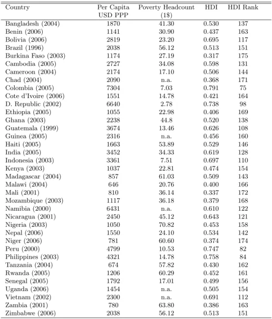
In the sample of countries we analyze in this paper, a large heterogeneity in terms of their level of human development is observable. Table 2 shows an overview of selected indicators of human development for the latest survey year for each country. Table 2 shows large country specific differences in the level of per capita GDP and poverty rates. The level of GDP per capita ranges from 646 USD PPP in Malawi (2004) to 7304 USD PPP in Colombia (2005). On average, low levels of GDP per capita correlate strongly to high rates of poverty. In addition, low levels of GDP per capita and high poverty rates are strongly related to a low level of human development measured by the Human Development Index (HDI). The values of the HDI show that no country in our sample belongs to the group of high human development (HDI≥0.8). In contrast, from the 37 countries in the sample, 16 countries are considered as countries with low human development showing a HDI of <0.5.9 All these countries are in Sub Sahara Africa. The other six Sub-Saharan African
coun-9
In particular, these countries are: Benin, Burkina Faso, Chad, Cote d’ Ivoire, Ethiopia, Guinea, Kenya, Malawi, Mali, Mozambique, Nigeria, Niger, Tanzania, Rwanda, Senegal, and Zambia.
tries exhibit an HDI value of around 0.5. The next group of similar human development with HDI values of slightly above the 0.5 threshold of low human development covers countries from Sub-Saharan Africa, Latin America, South Asia, and the Caribbean.10 No country in Sub-Sahara Africa has a HDI value of more than 0.610 (Namibia). The third group is characterized by HDI val-ues that range between 0.6 and 0.75 showing the highest human development in our sample.11 All these countries are from Latin America or South Asia.
Among all countries, Burkina Faso shows the lowest HDI of only 0.317, whereas Colombia shows the highest value of the HDI with 0.791. The heterogeneity of the countries is also reflected by the HDI ranks of the countries. The position varies from 75 (Colombia) to 175 (Burkina Faso) from 177 listed countries in the Human Development Reports.
After showing the large differences in the level of human development be-tween countries, we now analyze the bebe-tween and within country differences in the access to the education system and in outcomes of education. Figure 1 provides an overview of the between and within country distribution of net attendance of primary education for the children in the respective official age range by asset index quintiles as well as the mean value for each country.12
First, looking at between country and region specific differences, Figure 1 shows large disparities in net attendance rates between countries and regions in the developing world. Some countries show a mean net attendance rate of more than 90 percent (i.e. Brazil, Vietnam, Indonesia, Colombia, Peru, Philippines). These high levels of access to the educational system confirm the relatively high levels of human development of these countries. One exception is Brazil. Although Brazil has a relatively low HDI value of 0.531 it shows the highest mean net attendance rate in primary education in our sample. In contrast, the countries with the lowest levels of human development also show the lowest attendance rates for primary education. For example, Burkina Faso, the country with the lowest HDI value, also exhibits the lowest level
10
In particular, these countries are: Bangladesh, Brazil, Cameroon, Ghana, Haiti, Mada-gascar, Uganda, and Zimbabwe.
11
In particular, these countries are: Colombia, Dominican Republic, Guatemala, Indone-sia, Nicaragua, Peru, Philippines, and Vietnam
12
For the official age ranges for primary and secondary education, see again Table A1 in the Appendix.
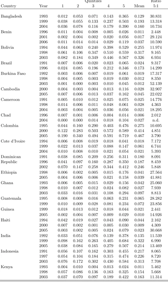
of net attendance in primary education. The group of Sub-Saharan African countries that were identified as countries with an HDI value of less than 0.5 also have the lowest net attendance rates in primary education. Whereas the richer countries show attendance rates of more than 90 percent, these countries have attendance rates of under 50 percent, reflecting large between country differences. This is also shown in Table 3, which shows the respective numbers to Figure 1, i.e. the net attendance rates in primary education by asset index quintiles and the mean value. Looking at the latest available survey year, one can also see the high between country differences by comparing the mean values between countries of different levels of human development. Colombia (2005) exhibits a mean net attendance rate of 94 percent, whereas Burkina Faso (2003) exhibits a rate of only 35 percent which is more than 2.5 times less than in Colombia. Furthermore, large differences in net attendance are also found between countries that are otherwise in a similar stage of human development. For example, Figure 1 and Table 3 show that although Kenya is at the same level of human development as Nigeria, Kenya has a significantly higher level of net attendance (0.884 compared to 0.689 in 2003). The same holds also, for example, for Bolivia and Vietnam. Besides the large country specific differences, one can clearly observe region specific differences in the level of access to the education system. Countries in Latin America and Asia exhibit an overall higher level of attendance rates than countries in Africa.
To confirm the result that the level of access to education is related to level of human development, Figure 2 shows the correlation between the net atten-dance rates in primary education and the HDI value for the latest available survey year for the countries in the sample. The figure shows a quite close re-lationship between the level of human development measured by the HDI and the access to the education system of children in the respective age cohort.
Similar between country and regions specific differences can also be ob-served when looking at the educational outcomes of adults. Figure 3 shows the percentage of primary education completion of adults aged between 23 and 27 by asset index quintiles as well as the country mean values for the respective latest available survey years for each country. Overall, Figure 3 conforms the results of Figure 1. Again, the countries with the lowest levels of human
devel-opment, i.e. the region of Sub-Saharan Africa, also show the lowest educational outcomes. Again countries from Latin America and Asia have, on average, a higher level of educational outcomes than countries from Africa. Interesting to note is that between country differences with respect to primary education completion rates are even higher than those with respect to net attendance rates. In fact, rates of primary education completion range from 89 percent in Indonesia (20003) to 12 percent in Mali (2001).13
Comparing the different indicators of access to education and educational outcomes with each other, Figure 4 presents the correlation between selected educational indicators by countries for the respective latest available survey year. Figure 4 shows a quite close relationship between educational indicators both for adults and children. For example, with increasing net attendance rates in primary education the years of education of adults also increase.
Tables 4-5 and Tables A2-A8 in the Appendix present the respective num-bers of all other educational indicators by asset index quintiles as well es the means for the latest available survey year, i.e. net attendance rates for sec-ondary education, average years of education for the agegroup 17-22 and 23-27, primary education completion rates (agegroup 17-22 and 23-27), secondary education completion rates (agegroup 17-22 and 23-27), and higher education completion rates (agegroup 17-22 and 23-27). All tables confirm the foregoing results of between country and region inequality in education.
5.2 Within Country Educational Inequality
One strong advantage of the use of household data in contrast to aggregated data sets for countries is the possibility to analyze differences within coun-tries between certain subgroups. In fact, our results point to very significant inequalities in education within most countries. This is for example demon-strated by Figure 1, which illustrates the disparities in net attendance rates in primary education between the richest and the poorest asset index quintile. Figure 2 shows that in many countries, there seem to be different worlds with respect to the distribution of access to education between welfare subgroups. Overall, within country inequality in access to education exhibits a similar
13
pattern to between country inequality. First, countries with lower levels off human development show the highest inequalities in net attendance rates in primary education, whereas in richer countries the inequality is significantly lower. Again, countries from Sub-Sahara Africa show higher levels of inequal-ity than countries from Latin America and Asia. Second, what is interesting to see is that educational inequality increases with lower average levels of net attendance rates.
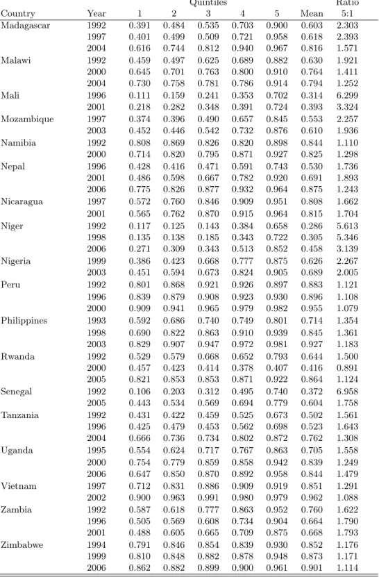
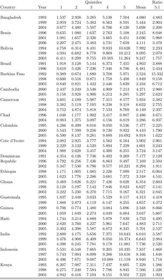
Table 3 concretizes the within country differences. Besides the distribution of net attendance rate over asset index quintiles, Table 3 also provides the ratio of the fifth to the first quintile as a direct indicator of inequality between the richest and the poorest population subgroup. Starting with the first country in Table 3, Bangladesh, it is shown that inequality in net attendance rates is quite low in Bangladesh. In the 2004, 80.8 percent of all children in the official primary education age range were enrolled in school in the poorest quintile, whereas 89 percent were enrolled in the richest quintile leading to a five to one ratio of 1.103. This result confirms the picture of Figure 3. However, when looking, for example, at the five to one ratio in net attendance in Niger in the year 2006, the result is very different. Here, the net attendance rate for the richest population quintile is more than three times higher than the net attendance rate of the poorest quintile (3.139).
Figure 3 and Tables 4 and 5 show the results for rates of primary education completion (agegroup 23-27), average years of education (agegroup 17-22) and secondary education completion (agegroup 17-22), respectively. Figure 3 shows that the within country inequalities for the indicators of educational outcomes are even higher than for net attendance rates as an indicator for the access to the education system. Again, inequality seems to increase with lower levels of educational attainment. But even countries with a relatively high level of primary education completion exhibit considerable within country disparities. The respective numbers for each quintile and the five to one ratios are shown in Table A5. For example, whereas the five to one ratio in Indonesia is 1.314 in the year 2003, the ratio in Ethiopia is 10.571 meaning that in Ethiopia the richest population quintile has a rate of primary education completion that is more than ten times higher than the rate for the poorest quintile. In addition, this
results also show that inequality in primary education completion between the poor and rich is about nine times higher in Ethiopia than in Indonesia. Table 4 also confirms the high differences in educational outcomes within countries and also the large between country differences in the level of educational inequality. For example, individuals in the richest quintile in Burkina Faso in the year 2003 aged between 17 and 22 have, on average, 6.712 times the years of education than those among the poorest population quintile (0.840 compared to 5.639). In addition, Table 4 again illustrates the between country differences in the outcomes of education. Even if inequality within the country is nearly at the same level like in Colombia (2005) and Malawi (2001), there remains a significant difference in the mean educational outcomes, which is almost a difference of three years.
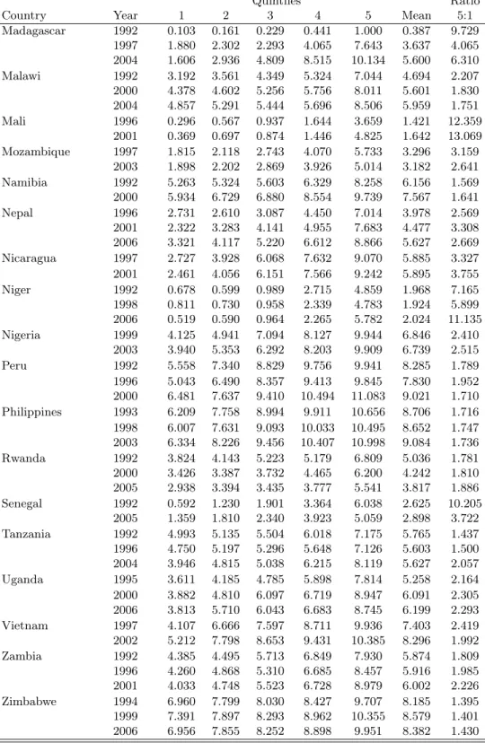
The differences in the level of educational outcomes and in the level of inequality within countries is even higher when it comes to higher levels of education. Looking at differences in secondary education completion between population welfare subgroups, which are presented in Table 5 for the agegroup 17-22 and in Table A6 for the agegroup 23-27, we also find dramatic disparities between the poorest and the richest quintile in nearly all countries. For exam-ple, whereas the ratio between the poorest and the richest quintile in primary education completion in Uganda (2006) was 3.323 (Table A3) it was 9.443 in the same year for secondary education completion among the individuals ages between 17 and 22 (Table 5). Table 5 also shows that in many countries the poorest quintile show rates of secondary education completion of the age-group 17-22 that are below 1 percent or even zero (like in Chad (2004)). And even more extreme inequalities are found when looking at the levels of higher educational outcomes, which are shown in Tables A7-A8. Higher education completion still remains a privilege for individuals living in countries with an overall higher development. Almost all African countries show levels of higher education below 1 percent among the first to third welfare quintile for both agegroups. As a result, many countries show ratios of the fifth to the first quintile of more than 10 (see Table A7 and A8).
To get a closer view on the distribution of access to education and ed-ucational outcomes, Figure 4 plots the distribution of net attendance rates,
years of education, and rate of primary education completion for Indonesia (for the years 1991, 1997, and 2003) and Burkina Faso (for the years 1993, 1998, and 2003). Figure 4 shows two main results: First, looking at the ed-ucational distribution of both countries, one can see a clear bias against the poor. For all indicators, the curves show a positive slope indicating that richer population subgroups have better access to education and higher educational outcomes than poorer population subgroups. Especially the first three vin-tiles are bypassed by access to education and educational outcomes. Then, all curves began to rise sharply illustrating the high disparities between the richest and the poorest welfare groups, which is particularly high in Burkina Faso. Second, looking at the differences between countries, Figure 4 illustrates again the large differences in access to educational and educational outcomes between countries. For all educational indicators, Indonesia shows a higher level than Burkina Faso in all periods. What is also interesting to note is that whereas significant differences in the levels of net attendance rates of primary and secondary education are found for both countries, the differences are much smaller when comparing educational outcomes of the two agegroups. The two countries are chosen es examples, because they illustrate the overall trend that we have found for the other countries in the sample, for which Figures A1a-A37a show the respective graphs by country and year in the Appendix. Also these Figures not only show the huge inequalities within countries but also huge disparities in inequality between countries and region, and not only in mean values as found in the previous section.
To show the relationship between the educational indicators within coun-tries, Figure 5 shows the correlations between several indicators by country for the latest available survey year. Overall, Figure 5 confirms the finding of a close relationship between educational indicators. For example, looking at the correlation between the net attendance rate of primary education and years of education, Figure 5 shows a quite clear relationship over the countries in the sample. In addition to the overall close relationship between educational indicators across countries, Figure 6 illustrates the relationship between the level of education and the level of within country inequality by showing the correlation between the net attendance rate of primary education completion
and between the net attendance rate of the poorest quintile, the richest quin-tile and the five to one ratio. Also Figure 6 confirms the foregoing results. In countries with high levels of attendance, also the poorest quintile show higher levels of attendance. However, Figure 6 also shows that countries with higher overall net attendance rate have also higher levels of inequality measured by the five to one ratio.
5.3 Pro-Poor Educational Progress?
We know analyze the trends in improvements of access to education and in educational outcomes over time and turn to the research question if and to what extent the progress in educational indicators have been pro-poor or not. For this, Figure 7 shows the non-income growth incidence curves (NIGIC) for the rates of net attendance in primary and secondary education, for years of education and primary and secondary education completion for the agegroups 17-22 and 23-27 for Indonesia (for the periods 1991-1997 and 1997-2003) and for Malawi (for the periods 1992-2000 and 2000-2004). For all other countries in the sample, the graphs are presented in Figures A1b-A38b in the Appendix. For the countries in the sample for which three surveys are available two NIGIC are presented, one for the pre-Dakar period and one for the post-Dakar pe-riod.14 For the other countries, one NIGIC is presented for the time between
between the respective two periods. Starting with Malawi (1992-2000), the NIGIC for net attendance in primary and secondary education show an overall pro-poor progress. Both curves are above zero along the whole distribution indicating an overall improvement in the net attendance rates in primary and secondary education. Both curves are also negatively sloped meaning that the growth rate in net attendance rates are higher for the poor than for the non-poor population subgroups. The same holds also, but to a lesser extent, for Indonesia (1991-1997). Also here, both curves are above zero and slightly negatively sloped. What is interesting to note here is that the very poor do not have made improvements in the net attendance in secondary education at all and that highest improvements have been made by the middle population vin-tiles. Looking at the post-Dakar period, the picture only slightly differs from
14
Since most surveys do were not available exactly for 1991, 1999 and later, we try to the two periods as close as possible to pre 1999 and post 1999.
the pre-Dakar period. Improvements in net attendance rates have been more equally distributed across the welfare distribution both in Malawi (2000-2004) and Indonesia (1997-2003). And although both NIGIC for Malawi are slightly negatively sloped, for some population subgroups, the situation has even been worsening especially middle of the welfare distribution.
Looking at the pre- and post-Dakar trends in changes in average years of education, Figure 7 shows a similar picture for educational outcomes of adults as for access to education. Although much more volatile than in the pre-Dakar period, for Malawi, both NIGIC show a pro-poor progress in the years of education in both periods for both agegroups. However, as already observed for Indonesia, also the very poor in Malawi have been bypassed by improvements in years of education in the post-Dakar period. And concerning adult education, it is interesting to see that improvements in Malawi in the post-Dakar are slightly higher for the agegroup 23-27, whereas in Indonesia it is slightly higher for the agegroup 17-22.
The next four curves present the NIGIC for rates of primary and secondary education completion for both agegroups and countries. Looking at the devel-opment of primary and secondary education completion in Mali during the pre-Dakar period, Figure 7 shows an overall positive and pro poor progress in primary education completion. Here, the highest growth rates are found for the very poor population subgroups. However, from the NIGIC for sec-ondary education completion it is not possible to draw any conclusions about the pro-poorness of the changes. For the first 7 vintiles, no growth rates are computable. The reason for this is that that the population subgroups at the lower end of the distribution had no secondary education completion in 1992 resulting in uncomputable growth rates, which is confirmed when looking and the first and second quintile for Malawi in Table 5. Table 5 also shows that even in 2000 very poor have almost no secondary education completion indi-cating an progress that was no pro-poor at all. For Indonesia (1991-1997), Figure 7 shows a slightly pro poor development for primary education com-pletion, whereas no clear trend is observable for secondary education. During the post-Dakar period both countries show improvements in primary and sec-ondary education completion, which are almost equally distributed across the
welfare groups. Thus, no clear evidence can be observed indicating pro-poor progress. Whereas highest rates of growth are found for the poorer welfare in Malawi (2001-2004), in Indonesia, again the middle of the distribution have benefited most from improvements. Also Table 5 confirms that improvements in both country are very low in secondary education completion.
The last four curves of Figure 7 show the development of years of education based on the unconditional ranking of individuals in the surveys. This means that the individuals are ranked by the years of education. The unconditional NIGIC, therefore, shows how the improvements in education are distributed over the education distribution, i.e. whether the education poor have been benefited overproportionally more from progress in education than the educa-tion richer groups. For the pre-Dakar period, Figure 7 shows only a very low progress at all. Very interesting to note is that the first five vintiles in Mali do not show any growth rates. This is because these population groups have had no education in the base year resulting in uncomputable growth rates. This finding is confirmed for almost all Sub-Saharan African countries.15 This holds also for the very poor subgroups in Indonesia, but to a lesser extent. Progress in educational outcomes was higher during the post-Dakar period. However, for Mali no real trend is observable that the education poor have been made higher progress than the non-poor. This is a very interesting result, because a slightly pro-poor development in the years of education was found for the conditional NIGIC, which shows the differences in both rankings and indi-cates that there is not a perfect correlation between education and welfare. In contrast, Indonesia show a more clear pro-poor development in educational outcomes.
When looking at the NIGIC of the other countries in the sample in the Appendix, no clear trend is observable concerning the pro-poorness of changes in access to education and in the educational outcomes. Overall, we find that Sub-saharan Africa is making progress but still lacks behind. For some coun-tries such as Cameroon, Colombia, and India, a pro-poor progress is observed for some indicators, whereas some countries like Ghana and Zambia even show an anti-poor development in education. For other countries the progress is
15
more or less equally distributed over the population such as in Cote D’Iviore, Dominican, Republic, Kenya, Nepal and Philippines. Moreover, there is also no clear common trend across the indicators we have analyzed within countries, nor between regions. For example, whereas in Niger a pro-poor development is found for the net attendance rate, an anti-poor development is found when looking at educational outcomes like years of education (see Figure A18b).
Concerning the research question about the differences in pro-poor progress between the pre-Dakar and post Dakar periods, we use Table 4, Table 3 and Table 5 to show the overall development in the mean values in access to ed-ucation and in eded-ucational outcome. The mean development already provide some interesting findings. For most countries, an overall positive development in education is observed. However, for some countries (among those for which we have three surveys) we observe a decrease in access to education during the pre-Dakar periods and then a rise in the post-Dakar period that is not high enough to compensate the foregoing decline. For example, whereas the mean in years of education in Burkina Faso decreased from 2.524 in 1992 to 1.849 in 1998, it increased to 2.234 in 2003 that is a lower mean level than in 1998.
Figure 8 provides an overview about the differences in the direction and ex-tent of changes in net attendance rate five to one ratio for all countries between the pre-Dakar and post-Dakar period. Also here, no clear trend is observable. For example, in Benin inequality in net attendance rate has been falling in both periods, and to a higher extent in the post-Dakar period. Starting from the vertical line to the arrow marked by ‘pre’ shows the change during the pre-Dakar period, which shows a decrease in inequality. From the ‘pre’ ar-row to the ‘post’ arar-row captures the changes during the post-Dakar period, which shows also a decrease that is higher than during the pre-Dakar period. Countries, in which inequality has decreased in both periods are Dominican Republic, Colombia, Cameroon, Burkina Faso, Benin, Bangladesh, Zimbabwe, Philippines, Nigeria, Malawi. Countries, in which the reduction in inequal-ity is higher for the post-Dakar periods are Cameroon and Nigeria. For some countries, inequality have been risen during the first period and fallen during the second period and vice versa (e.g. Haiti and Rwanda). Overall, Figure 8 confirms the foregoing result that no clear country specific, region specific
or period specific trends are observed in the pro-poorness of the changes in education.
5.4 Inequality in Education by Gender and Areas
After having analyzed the pro-poor progress in access to education and in educational outcomes between countries and within countries across welfare groups, we now turn to the analysis of differences on pro-poor progress in education by gender and by rural and urban areas.
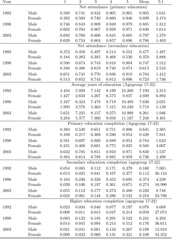
Table 6 and Figure 9 show the differences in the educational indicators by gender exemplarily for India. For all indicators and periods, three glaring findings emerge. First, the level of access to education and of educational outcomes are considerably higher for boys than for girls, not only on average but also for every single asset index quintile. For example, whereas the net attendance rate in secondary education of the boys in the poorest quintile was 65 percent in 2003 it was only 51 percent for the girls. A boy of the poorest quintile have had almost twice as much years of education than girls in 2003 (5.651 compared to 3.284). The gender bias in education is worse for higher education. Girls of poorer welfare subgroups in India are almost perfectly bypassed by access to higher education completion resulting an very low rates higher educational outcomes.
Second, gender specific inequality in education is higher for the poor than for the non-poor. This is illustrated by Figure 9, which shows not only the dif-ferences in the level of education between boys and girls but also an increasing convergence of the curves with increasing welfare. Especially when looking on adult education, gender specific inequality in education is first of all a problem for the poor. In richer welfare groups, the one who can afford the costs of education for all children, a gender bias in education diminishes.
Third, inequality between welfare groups is higher for girls education than for boys education. The five to the one ratio is significantly higher for girls than for boys for all indicators and periods in India.
To analyze the pro-poor progress separately for males and females, Figure 10 shows the NIGIC by gender for India. Overall, we found that improvements in the access to education and in educational outcomes were pro-poor in India
in the pre-Dakar period as well as in the post-Dakar period. For all indicators, there is also a pro-poor development for boys and for girls. Interesting to observe is that for net attendance rates in primary education, years of schooling and primary education completion, the growth rates for girls are higher than for boys, especially at the lower end of the distribution. This is a very promising results, indicating a decrease in gender inequality in education. This is also confirmed by Table 6, which shows that the absolute differences between girls and boys decreases over the years. The low growth rates at the upper end of the distribution indicates that these welfare groups have had already a high level of education so that remains only limited potential for further improvements. For education of adults, Figure 10 shows that again, the poor are bypassed by improvements in education. In the pre-Dakar period, especially the middle of the distribution have been benefited from improvements, whereas the progress was very small and slightly anti-poor during the post-Dakar period.
However, overall, we found that gender differences in education are charac-teristic for countries with low overall attendance. Besides the positive develop-ment in India, underparticipation in education of girls is a persisting concern in Sub-saharan African countries. This regions show no real progress in achieving gender parity.
Table 7 and Figure 11 show the differences in access to education and in educational outcomes between rural and urban areas in Burkina Faso, which mirrors the overall trend across the countries in the sample. As expected, access to education and educational outcomes are much higher in urban areas than in rural areas. Children from rural households are less likely to be attended than children living in urban areas. This is illustrated in Figure 11 for the year 2003. Although the curves show a similar pattern across the distribution, one can see the large difference in the level of access to education between rural and urban areas.
Table 7 shows that whereas the mean years of education in 2003 was 5.503 years for the agegroup 17-22 in urban areas, it was only 1.248 in rural areas. In addition, higher levels of educational outcomes are very low in rural areas. The same trend is found for all other education indicators.
distribution, two main findings emerge. First, inequality in education is higher in rural areas than in urban areas. For example, whereas the five to one ratio for primary education completion in 2003 is 1.799 in urban areas, it was 4.299 in rural areas. Second, differences in education between urban and rural areas are higher for the poor than for the non-poor. For example, the urban rural ratio in years of education in 2003 was 7 for the poorest asset index quintile, for the richest quintile it was 2.9.
Figure 12 shows the pro-poor progress in education in Burkina Faso by urban and rural areas. Besides an overall increase in the access to education and also in educational outcomes, subnational disparities remain between ur-ban and rural areas in both periods. For the post-Dakar period, growth rates are slightly higher for rural areas indicating a small decrease in inequality be-tween rural and urban areas. However, the unconditional NIGIC shows that the education poor in rural areas have not benefitted more from improvements in education than the education poor in urban areas. These results are also confirmed by the other countries in the sample. The improvements that have been made are more or less equally distributed across welfare groups and also across regions. This means that, as also found for gender parity in education, large differences in education between rural and urban areas remain.
6
Concluding Remarks
The question whether the poor can benefit from progress in access to the education system and educational outcomes is of considerable importance with respect the achievements of the EFA goals until 2015. The aim of the paper was to identify and understand which parts of the population have benefited most or have not benefited from the improvements in the access to the education system and in educational outcomes and to highlight the differences in the progress, if any, between the pre- and post-Dakar periods.
In this paper we provided a synthesis of the distribution, and changes in ac-cess to education and in education outcomes over-time by welfare, gender and urban and rural areas for 37 developing countries. In particular, we calculated the distribution of net attendance rates in primary and secondary education, years of schooling and rates of primary, secondary and higher education
com-pletion across the welfare distribution based on the asset index for each country and period, and provided also a pro-poor progress analysis of changes in the indicators over time.
Overall, our findings confirm that the level of access to education is related to level of human development. The countries with the lowest levels of human development, i.e. the region of Sub-Saharan Africa, also shows the lowest educational outcomes. We also find considerable region specific differences in the access to education and in educational outcomes. Countries from Latin America and Asia have, on average, a higher level of educational outcomes than countries from Africa.
Concerning within country differences in education by welfare, our results point to very significant inequalities in education within most countries. Richer population subgroups have better access to education and higher educational outcomes than poorer population subgroups. Within country inequality in access to education exhibits a similar pattern to between country inequality. First, countries with lower levels off human development show the highest inequalities in education, whereas in richer countries, the inequality is signifi-cantly lower. In addition, educational inequality increases with lower average levels of education, while we find a close relationship between educational in-dicators. Furthermore, the differences in the level of educational outcomes and in the level of inequality within countries are even higher when it comes to higher levels of education.
Concerning the question if and to what extent the progress in educational indicators have been pro-poor or not and concerning the research question about the differences in pro-poor progress between the pre-Dakar and post Dakar periods, we find that although positive average improvements have been made, in all countries over time, no clear country specific, region specific or pe-riod specific trend is observed in the pro-poorness of the changes in education. One alarming common finding is that although Sub-saharan Africa is making progress, it still lacks far behind other regions and behind the goals. Even more worrying is that the very poor population subgroups are often bypassed by improvements in education.
countries we find that, first, the level of access to education and of educational outcomes are considerably higher for boys than for girls and higher in urban than in rural areas. Second, gender specific and region specific inequality in ed-ucation is higher for the poor than for the non-poor. Third, inequality between welfare groups is higher for girls education than for boys education and also higher in rural than in urban areas. In addition, gender bias in education and regional differences are worse for higher education. Overall, we found that gen-der and region specific differences in education are characteristic for countries with low overall attendance. Besides overall positive development, underpar-ticipation in education of girls is a persisting concern in Sub-saharan African countries. This region shows no real progress in achieving gender parity. Large differences in education also remain between rural and urban areas.
References
Berthélemy, J.C. (2005), To what Extent are African Education Policies Pro-Poor?, Journal of African Economies, 15 (3): 434-469.
Bourguignon, F. and S. Chakravarty (2003), The Measurement of Multidi-mensional Poverty, Journal of Economic Inequality, 1: 25-49.
Chabbott, C. and F. O. Ramirez (2000), Development and education, in M. Hallinan (ed.), Handbook of the Sociology of Education, New York, Kluwer Academic.
Cornia, G.A. and L. Menchini (2007), Health Improvements and Health In-equality during the Laset 40 Years, in G. Mavrokas and A. Shorrocks (eds)Advancing Development - Core Themes in Global Economics, Helsinki: Wider.
Duflo, E. and L. Breierova (2002), The Impact of Education on Fertility and Child Mortality: Do Fathers Really Matter less than Mothers? Mas-sachusetts Institute of Technology, Department of Economics.
Filmer, D. and L.H. Pritchett (2001), Estimating Wealth Effects without Expenditure Data - or Tears: An Application to Educational Enrollments in States of India, Demography, 38 (1): 115-132.
Grimm, M. (2007), Removing the anonymity axiom in assessing pro-poor growth. With an application to Indonesia and Peru,Journal of Economic Inequality, forthcoming.
Grimm, M., C. Guénard, and S. Mesplé-Somps (2002), What has happened to the urban population in Côte d‘Ivoire since the eighties? An analysis of monetary poverty and deprivation over 15 years of household data,
World Development, 30 (6): 1073-1095.
Grosse, M., K. Harttgen and S. Klasen (2008), Measuring Pro-Poor Growth using Non-Income Indicators, World Development (forthcoming). Hanmer, L. and D. Booth (2001), Pro-Poor Growth: Why do we need it?,
Klasen, S. (2008), Economic Growth and Poverty Reduction: Measurement Issues in Income and Non-Income Dimensions,World Development (forth-coming).
Klasen, S. (2004), In Search of the Holy Grail: How to Achieve Pro Poor Growth?, in Tungodden, B., N. Stern, and I. Kolstad (eds) Toward Pro Poor Policies-Aid, Institutions, and Globalization, New York: Oxford University Press.
Klasen, S. (2000), Measuring Poverty and Deprivation in South Africa,Review of Income and Wealth, 46 (1): 33-58.
Lanjouw, P. and M. Ravallion (1998), Benefit Incidence and the Timing of Program Capture, Washington, World Bank.
LeVine, R. A., S. E. LeVine, M. L. Rowe, and B. Schnell-Anzola (2004), Maternal literacy and health behavior: a Nepalese case study, Social Science and Medicine, 58: 866-877.
Milligan, K., E. Moretti, and P. Oreopoulos (2003), Does education improve citizenship? Evidence from the US and the UK, Journal of Public Eco-nomics, 88(9): 1667-1695.
Mukherjee, D. (2001), Measuring multidimensional deprivation,Mathematical Social Sciences, 42: 233-251.
OECD (2006), Promoting Pro-Poor Growth: Key Policy Messages, Paris: OECD.
OECD (2001), Rising to the Global Challenge: Partnership for Reducing World Poverty, Statement by the DAC High Level Meeting. April 25-26, 2001, OECD, Paris.
Ravallion, M. and S. Chen (2003), Measuring Pro-Poor Growth, Economics Letters, 78 (1): 93-99.
Ravallion, M. and G. Datt. (2002), Why has economic growth been more pro-poor in some states of India than others?, Journal of Development Economics, 68: 381-400.
Roberts, J. (2003), Poverty Reduction Outcomes in Education and Health: Public Expenditure and Aid, Overseas Development Institute Working Paper 210, ODI, London.
Sahn, D.E. and D. Stiefel (2003), Exploring Alternative Measures of Welfare in the Absense of Expenditure Data, Review of Income and Wealth, 49 (4): 463-489.
Schultz, P. T. (2002), Why governments should invest more to educate girls,
World Development, 30(2): 207-225.
Sen, A.K. (1988), The Concept of Development, in H. Chenery and T. Srini-vasan (eds) Handbook of Development Economics, Vol. 1, 9-26.
Sen, A.K. (1987),Standard of Living, New York: Cambridge University Press. Smits, J., J. Huisman, and E. Webbink (2007), Family Background, Dis-trict and National Determinants of Primary School Enrollment in 62 Developing Countries. Paper presented at the XIII World Congress of Comparative Education Societies, Sarajevo, 3-7 September.
Son, H. (2003), Approaches to Defining and Measuring Pro-Poor Growth, Mimeo, Washington, World Bank.
Summer, A. (2003), Economic and Non-Economic Well-Being: A Review of Progress on the Meaning and Measurement of Poverty, Paper Prepared for WIDER Conference: Inequality, Poverty and Human Well-Being, May 30-31, 2003, Helsinki.
UN (2007), The Millennium Development Goals Report 2007, New York: United Nations.
UN (2005), The Millennium Development Goals Report 2005, New York: United Nations.
UN (2000), A Better World for All, New York: United Nations.
UN (2000a), United Nations Millennium Declaration, A/RES55/2, New York, United Nations.
UNESCO (2007), Education for All by 2015 - Will we make it? EFA Global Monitoring Report 2008, Paris: UNESCO.
Van de Walle, D. (1998), Assessing the Welfare Impacts of Public Spending,
World Development, 26 (3): 365-379.
Van de Walle, D., and K. Nead (eds) (1995), Public Spending and the Poor - Theory and Evidence, published for the World Bank, Baltimore and London: John Hopkins University Press.
White, H. and E. Anderson (2000), Growth versus Distribution: Does the Pattern of Growth Matter?, Development Policy Review, 19 (3): 267-289.
World Bank (2000), World Development Report 2000 - Attacking Poverty, Washington: World Bank.
Tables and Figures
Table 1: Demographic and Health Surveys by Country and Years
Country Years Country Year
Bangladesh 1993, 1999, 2004 Brazil 1991, 1996
Benin 1996, 2001, 2006 Cambodia 2000, 2005
Bolivia 1994, 1998, 2003 Chad 1996, 2004
Burkina Faso 1992, 1998, 2003 Ethiopia 1998, 2005
Cameroon 1991, 1998, 2004 Guatemala 1995, 1999
Colombia 1995, 2000, 2005 Guinea 1999, 2005
Cote d’Ivoire 1994, 1999, 2004 Mali 1996, 2001
Dominican Republic 1991, 1996, 2002 Mozambique 1997, 2003
Ghana 1993, 1998, 2003 Namibia 1992, 2000 Haiti 1994, 2000, 2005 Nicaragua 1997, 2001 India 1992, 1999, 2005 Nigeria 1999, 2003 Indonesia 1991, 1997, 2003 Senegal 1992, 2005 Kenya 1993, 1998, 2003 Vietnam 1997, 2002 Madagascar 1992, 1997, 2004 Malawi 1992, 2000, 2004 Nepal 1996, 2001, 2006 Niger 1992, 1998, 2006 Peru 1992, 1996, 2000 Philippines 1993, 1998, 2003 Tanzania 1992, 1996, 2004 Rwanda 1992, 2000, 2005 Uganda 1995, 2000, 2006 Zambia 1992, 1996, 2001 Zimbabwe 1994, 1999, 2006