Volume 17 | Issue 1 Article 2
2018
Single missing data imputation in PLS-based
structural equation modeling
Ned Kock
Texas A & M International University, Laredo, [email protected]
Follow this and additional works at:https://digitalcommons.wayne.edu/jmasm
Part of theApplied Statistics Commons,Social and Behavioral Sciences Commons, and the
Statistical Theory Commons
This Invited Article is brought to you for free and open access by the Open Access Journals at DigitalCommons@WayneState. It has been accepted for
Recommended Citation
Kock, N. (2018). Single Missing Data Imputation in PLS-based Structural Equation Modeling. Journal of Modern Applied Statistical Methods, 17(1), eP2712. doi: 10.22237/jmasm/1525133160
Cover Page Footnote
The author is the developer of the software WarpPLS, which has over 7,000 users in more than 33 different countries at the time of this writing, and moderator of the PLS-SEM e-mail distribution list. He is grateful to those users, and to the members of the PLS-SEM e-mail distribution list, for questions, comments, and discussions on topics related to SEM and to the use of WarpPLS.
doi: 10.22237/jmasm/1525133160 | Accepted: December 5, 2017; Published: June 7, 2018. Correspondence: Ned Kock, [email protected]
Ned Kock is Killam Distinguished Professor and Chair of the Division of International Business and Technology Studies, A.R. Sanchez, Jr. School of Business, Texas A&M International University.
INVITED ARTICLE
Single Missing Data Imputation in
PLS-based Structural Equation Modeling
Ned Kock
Texas A&M International University Laredo, TX
Missing data, a source of bias in structural equation modeling (SEM) employing the partial least squares method (PLS), are commonly handled with deletion methods such as listwise and pairwise deletion. Missing data imputation methods do not resort to deletion. Five single missing data imputation methods are considered employing the PLS Mode A algorithm of which two hierarchical methods are new. The results of a Monte Carlo experiment suggest that Multiple Regression Imputation yielded the least biased mean path coefficient estimates, followed by Arithmetic Mean Imputation. With respect to mean loading estimates, Arithmetic Mean Imputation yielded the least biased results, followed by Stochastic Hierarchical Regression Imputation and Hierarchical Regression Imputation. Single missing data imputation methods perform better with PLS-SEM based on their performance with other multivariate analysis techniques such as multiple regression and covariance-based SEM.
Keywords: Partial least squares; structural equation modeling; missing data imputation; path bias; stochastic regression; Monte Carlo simulation
Introduction
The method of partial least squares (PLS) experienced explosive growth in the context of structural equation modeling (SEM), whereby latent variables are measured via indicators in questionnaires (Akter et al., 2017; Kock, 2016; Rigdon, 2016). Indicators frequently take the form of scores generated based on question-statements answered on Likert-type scales. PLS-SEM estimates latent variables
through composites, which are exact linear combinations of the indicators assigned to the latent variables (Kock, 2015a; 2015b).
A main source of bias in PLS-SEM is missing data (Newman, 2014). Among patterns of missing data, particularly common in behavioral research is that known as missing at random (MAR), which is actually a misnomer. This pattern occurs when the probability of a missing value is related to other measured variables, but unrelated to the underlying values of the variable that are missing. For example, if scores measuring the accuracy of a graphical representation are more likely to be missing for a certain type of representation than for others, then the corresponding missing data will follow the MAR pattern. Researchers have traditionally used deletion methods, often listwise and pairwise deletion (Enders, 2010). They are a source of error that may distort coefficients of association; where the error is introduced into the data as deletion occurs. For example, missing data may be associated with groups of respondents who share some characteristics, and whose exclusion from datasets can significantly influence the strength of relationships among variables. Deletion methods also reduce the sample size available for an analysis, and thus the statistical power of virtually any type of analysis applied to the data. Wilkinson (1999) opine these techniques are “among the worst methods available for practical applications” (p. 598).
Missing data imputation methods provide an alternative to deletion methods. Through imputation missing data elements are replaced with well-informed guesses, obtained through various algorithms, leading to no reduction in sample size. Five single missing data imputation methods are considered in the context of PLS-SEM, with MAR data, of which two are new.
Illustrative Model
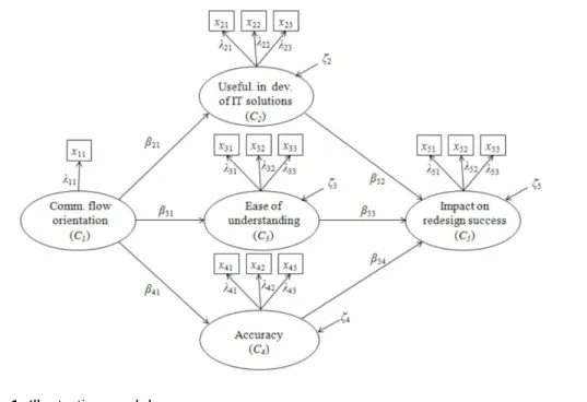
An illustrative model serves as the basis for a Monte Carlo experiment and empirical illustration. The illustrative model is depicted in Figure 1, and contains five latent variables, for which composites are estimated via PLS-SEM. The latent variables, which refer to theoretical constructs, are: communication flow orientation (C1), usefulness in the development of information technology (IT)
solutions (C2), ease of understanding (C3), accuracy (C4), and impact on redesign
Figure 1. Illustrative model
The mathematical symbols used in the model, and in the following sections, were adapted from the classic path analysis, covariance-based SEM, and PLS literatures (Kline, 2010; Kock, 2016; Lohmöller, 1989; Wright, 1934; 1960): βij is
the path coefficient for the link going from composite Cj to composite Ci, λij is the
loading for the jth indicator of composite Ci, and ζi is the structural error
associated with an endogenous composite Ci. With exception of communication flow orientation (C1), a set of indicators xij is used to measure each composite Ci.
When more than one indicator is used to measure a composite, each indicator is assumed to measure the composite with a certain degree of imprecision.
Communication flow optimization theory (Danesh-Pajou, 2005; Kock, 2003) is the foundation on which the illustrative model is built. Although this theory is not the focus of the investigation, it is useful to know its main prediction. A greater focus on how communication takes place in business processes, in redesign efforts, is associated with better business process redesign outcomes. Business process redesign efforts are aimed at improving the operations of organizations, regardless of size and industry. In them groups of employees and managers collaboratively analyze and redesign business processes, which are sets of interrelated activities (Kock, 2007; Mendling et al., 2012). Virtually any good
or service is produced in organizations via a business process – e.g., the process of assembling a car, carried out by an automaker.
Communication flow orientation (C1) is the degree to which a business
process modeling approach explicitly shows how communication interactions take place in a business process. This latent variable can be measured through a single indicator storing either 1 or 0, for a study contrasting two opposite modeling approaches, corresponding to a high or low communication flow orientation of a business process modeling approach used.
Usefulness in the development of IT solutions (C2) is the degree to which a
process modeling approach is useful in the development of a generic IT solution to automate the redesigned process. The need to automate redesigned processes with IT is almost universal in modern businesses. An example of question-statement that can be used for measurement of this latent variable is: “This process modeling approach is useful in the development of a generic IT solution to automate the redesigned process”.
Ease of understanding (C3) is the degree to which a process modeling
approach is perceived to yield a process representation that is easy to understand. An example of question-statement that can be used for measurement of this latent variable is: Processes modeled using this approach are easy to understand.
Accuracy (C4) is the degree to which a process modeling approach is
perceived to lead to an accurate representation of the process. An example of question-statement that can be used for measurement of this latent variable is: This process modeling approach leads to accurate process representations.
Impact on redesign success (C5) is the degree to which the process modeling
technique used is perceived to lead to an actual improvement of the targeted business process. An example of question-statement that can be used for measurement of this latent variable is: Using this process modeling approach is likely to contribute to the success of a process redesign project.
Missing Data Imputation Methods Analyzed
All variables are assumed to be standardized. This has no effect on the implementation of the methods; the methods can take as inputs unstandardized variables, store means and standard deviations for later unstandardization, standardize the variables, apply the various operations that define the methods, and finally unstandardize the variables again prior to generating the outputs.
Arithmetic Mean Imputation
Let xi be a column vector denoting one of the k manifest variables used in a SEM model. The Arithmetic Mean Imputation (MEAN) method assigns values to each missing element xir according to (1), where Nm is the number of missing values in
xi, and xi is the arithmetic mean of variable xi.
,
ir i
x =x (1)
1 m.
r= N
The Arithmetic Mean Imputation (MEAN) method replaces each missing element xir in a column of data i within a dataset, which refers to a manifest variable, with the average (or arithmetic mean) of that column. This method is the simplest of the imputation methods discussed here. Although it can be employed by itself, this method also plays an ancillary role in other methods.
Multiple Regression Imputation
The Multiple Regression Imputation (MREGR) method assigns values to each missing element xir according to (2), where k is the number of manifest variables used in a model, Nm is the number of missing values in xi, and each of the
elements of the matrix of estimated regression coefficients ˆ i j
x x
is calculated through a multiple regression analysis with xi as the criterion and
xj(j = 1 … k, j ≠ i) as the predictors. 1 ˆ , i j k ir j x x jr x =
= x (2) 1 , , 1 m. j= k ji r= NIn the Multiple Regression Imputation (MREGR) method each missing element xir is replaced with the corresponding expected value of xi given all of
the other variables xj(j = 1 … k, j ≠ i) in the dataset. The regression coefficients ˆ
i j
x x
for each variable xi are obtained via a multiple regression analysis after an
An alternative to using Arithmetic Mean Imputation (MEAN), which tends to lead to an exacerbation of the biases and that is therefore not employed here, is to conduct the multiple regression analysis to obtain the regression coefficients
ˆ i j
x x
after a listwise deletion. The use of deletion is particularly problematic here because the regression equation will typically have quite a few predictors, and thus a great deal of data may end up being lost after a listwise deletion.
Hierarchical Regression Imputation
The Hierarchical Regression Imputation (HREGR) method, a new method, assigns values to each missing element xir according to (3), where k is the number of manifest variables used in a model, Nm is the number of missing values
in xi, and each of the elements of the matrix of estimated correlations ˆ
i j
x x is calculated after a pairwise deletion of missing elements is conducted for each pair of variables xi and xj. In this equation max
( )
ˆi j
x x
is the maximum estimated correlation between the manifest variable xi and any other manifest variable xj for
which a corresponding non-missing value xjr exists.
( )
ˆ max , i j ir x x jr x = x (3) 1 , , 1 m. j= k ji r= NIn the Hierarchical Regression Imputation (HREGR) method each missing element xir is replaced with the corresponding expected value of xi given a variable xj, stored in column j of the dataset, where xj is the variable with the
highest correlation with xi after a pairwise deletion of missing elements.
A pairwise deletion is preferred over an Arithmetic Mean Imputation (MEAN) for the calculation of the correlations ˆ
i j
x x
because it leads to less bias, as indicated by exploratory versions of this method that we developed and tested. In datasets with multiple variables and widespread missing data elements, pairwise deletions usually lead to much lesser amounts of data loss than listwise deletions. Nevertheless, the results of analyses conducted after pairwise deletions tend to be dependent on the pair-specific idiosyncrasies of missing data patterns.
Stochastic Multiple Regression Imputation
The Stochastic Multiple Regression Imputation (MSREG) method assigns values to each missing element xir according to (4), where k is the number of manifest variables used in a model, Nm is the number of missing values in xi, and
Srandn(⬚) is a function that returns a different element of a standardized normally distributed random column vector each time it is invoked.
(
)
1 1 ˆ 1 ˆ ˆ i j i j i j k k ir j x x jr j x x x x x = = x + − = Srandn
(⬚), (4) 1 , , 1 m. j= k ji r= NThe Stochastic Multiple Regression Imputation (MSREG) method is similar to the Multiple Regression Imputation (MREGR) method. The key difference is that in this stochastic variety, implemented via the equation above, normal random error is added to the new values due to the assumption that not doing so can create a downward bias in standard errors. Such a bias could lead to an exacerbation of Type I errors. The random error elements yielded by Srandn(⬚) are weighted so that they collectively account for all of the variance in xi that is
not explained by the predictors xj (j = 1…k, j ≠ i).
Although the above assumption regarding standard error bias may be a reasonable one with respect to standard multiple regression and covariance-based SEM, in PLS-SEM path coefficients tend to present downward biases even without missing data. Therefore, a downward bias in standard errors may compensate for the related decrease in statistical power, due to the downward path coefficient bias, in turn countering an exacerbation in Type II errors (and a reduction in power).
Stochastic Hierarchical Regression Imputation
The Stochastic Hierarchical Regression Imputation (HSREG) method, another new method, assigns values to each missing element xir according to (5), where k is the number of manifest variables used in a model, Nm is the number of missing
values in xi, and Srandn(⬚) is a function that returns a different element of a
( )
( )
2 ˆ ˆ max 1 max i j i j ir x x jr x x x = x + − Srandn (⬚), (5) 1 , , 1 m. j= k ji r= NThe Stochastic Hierarchical Regression Imputation (HSREG) method is similar to the Hierarchical Regression Imputation (HREGR) method. The key difference (analogously to the discussion above) in this stochastic variety is that normal random error is added to the new values due to the assumption that not doing so can create a downward bias in standard errors and an overall deleterious effect on type I error rates. Although this assumption may find general application in standard multiple regression and covariance-based SEM, it may not readily apply to PLS-SEM.
Monte Carlo Experiment
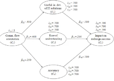
A Monte Carlo experiment based on the true population model shown in Figure 2 was conducted to assess the performance of the five missing data imputation methods discussed in the previous section. Performance was assessed in terms of path coefficient bias and standard error inflation.
When creating data for our Monte Carlo experiment we varied the following conditions: percentage of missing data (0%, 30%, 40%, and 50%), and sample size (100, 300, and 500). This led to a 4 × 3 factorial design, with 12 conditions, where 1,000 samples were analyzed for each of these 12 conditions for a total of 12,000 samples.
The PLS Mode A algorithm with the path weighting scheme (Lohmöller, 1989) was used in the analyses. These are the most widely used algorithm (PLS Mode A) and inner model estimation scheme (path weighting) in the context of PLS-SEM. Results were obtained for analyses with no missing data (NMD), Arithmetic Mean Imputation (MEAN), Multiple Regression Imputation (MREGR), Hierarchical Regression Imputation (HREGR), Stochastic Multiple Regression Imputation (MSREG), and Stochastic Hierarchical Regression Imputation (HSREG).
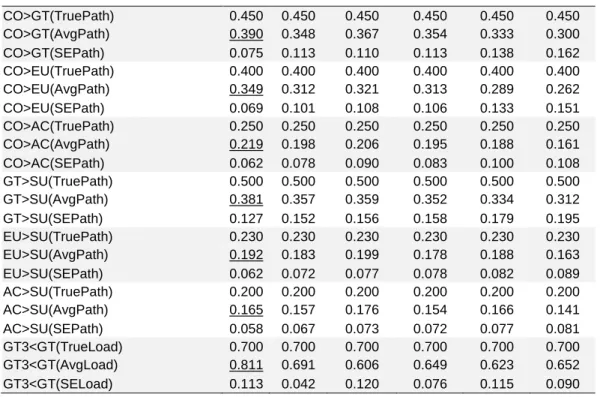
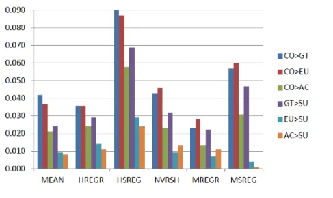
A summarized set of results are shown in Table 1 and Figure 3, where N = 300 and 30% missing data (MAR). In the figure, consider the absolute path coefficient differences with respect to no missing data (NMD) estimates, to highlight the performance of the various missing data imputation methods. In the table, true path coefficients, mean path coefficient estimates, and standard errors of path coefficient estimates are shown next to one another. Full results, for all percentages of missing data and sample sizes included in the simulation, are available in Appendix A. Because all loadings are the same in the true population model, loading-related estimates for only one indicator of the composites are shown. This avoids crowding and repetition, as the same pattern of results repeats itself in connection with all loadings.
The mean path coefficient estimates that are shown underlined in the table were obtained through the application of the PLS Mode A algorithm to datasets where no data was missing (NMD). Note that they generally underestimate the true path coefficients. This underestimation stems from the use of composites in PLS-SEM, discussed earlier, which leads to an attenuation of composite correlations (Nunnally & Bernstein, 1994). This correlation attenuation extends to the path coefficients (Kock, 2015b), leading to the observed underestimation. The opposite effect is observed in connection with loadings, which tend to be overestimated in PLS-SEM.
Multiple Regression Imputation (MREGR) yielded the least biased mean path coefficient estimates, followed by Arithmetic Mean Imputation (MEAN). When we look at mean loading estimates, Arithmetic Mean Imputation (MEAN) yielded the least biased results, followed by Stochastic Hierarchical Regression Imputation (HSREG) and Hierarchical Regression Imputation (HREGR).
Compared with the no missing data condition (NMD), none of the methods induced a significant bias in standard errors. This is noteworthy since prior results outside the context of PLS-SEM have tended to show a significant downward bias in standard errors, particularly for non-stochastic varieties. Such downward bias in standard errors has led to concerns regarding an inflation in type I errors, and warnings against the use of single missing data imputation methods in general (Enders, 2010; Newman, 2014).
Table 1. Summarized Monte Carlo experiment results (N = 300, 30% MAR data) Missing data imputation scheme NMD MEAN MREGR HREGR MSREG HSREG
CO>GT(TruePath) 0.450 0.450 0.450 0.450 0.450 0.450 CO>GT(AvgPath) 0.390 0.348 0.367 0.354 0.333 0.300 CO>GT(SEPath) 0.075 0.113 0.110 0.113 0.138 0.162 CO>EU(TruePath) 0.400 0.400 0.400 0.400 0.400 0.400 CO>EU(AvgPath) 0.349 0.312 0.321 0.313 0.289 0.262 CO>EU(SEPath) 0.069 0.101 0.108 0.106 0.133 0.151 CO>AC(TruePath) 0.250 0.250 0.250 0.250 0.250 0.250 CO>AC(AvgPath) 0.219 0.198 0.206 0.195 0.188 0.161 CO>AC(SEPath) 0.062 0.078 0.090 0.083 0.100 0.108 GT>SU(TruePath) 0.500 0.500 0.500 0.500 0.500 0.500 GT>SU(AvgPath) 0.381 0.357 0.359 0.352 0.334 0.312 GT>SU(SEPath) 0.127 0.152 0.156 0.158 0.179 0.195 EU>SU(TruePath) 0.230 0.230 0.230 0.230 0.230 0.230 EU>SU(AvgPath) 0.192 0.183 0.199 0.178 0.188 0.163 EU>SU(SEPath) 0.062 0.072 0.077 0.078 0.082 0.089 AC>SU(TruePath) 0.200 0.200 0.200 0.200 0.200 0.200 AC>SU(AvgPath) 0.165 0.157 0.176 0.154 0.166 0.141 AC>SU(SEPath) 0.058 0.067 0.073 0.072 0.077 0.081 GT3<GT(TrueLoad) 0.700 0.700 0.700 0.700 0.700 0.700 GT3<GT(AvgLoad) 0.811 0.691 0.606 0.649 0.623 0.652 GT3<GT(SELoad) 0.113 0.042 0.120 0.076 0.115 0.090
Notes: NMD = no missing data; MEAN = Arithmetic Mean Imputation; MREGR = Multiple Regression
Imputation; HREGR = Hierarchical Regression Imputation; MSREG = Stochastic Multiple Regression Imputation; HSREG = Stochastic Hierarchical Regression Imputation; XX>YY = link from composite XX to YY; CO = communication flow orientation (C1); GT = usefulness in the development of IT solutions (C2); EU = ease
of understanding (C3); AC = accuracy (C4); SU = impact on redesign success (C5); TruePath = true path
coefficient; AvgPath = mean path coefficient estimate; SEPath = standard error of path coefficient estimate; TrueLoad = true loading; AvgLoad = mean loading estimate; SELoad = standard error of loading estimate.
Figure 3. Absolute path coefficient differences with respect to no missing data (NMD) estimates
Empirical Illustration
Summarized in Table 2 are results of an empirical field study related to the illustrative and true population models discussed earlier. It served as the basis for the development of the illustrative and true population models. Shown next to one another are estimated path coefficients (top part of the table), and loadings (bottom part of the table). All path coefficients and loadings are shown. Except for the column “NMD”, all other columns show results with 30% missing data (MAR).
The data for this empirical study was collected from 156 individuals who participated in various business process redesign projects in organizations located in Northeastern U.S.A. The participants employed one of two business process modeling approaches. One of the modeling approaches focused primarily on the communication flow within business processes. The other focused primarily on the chronological flow of activities. Both approaches are illustrated in Appendix B. Appendix C has the questionnaire used for data collection.
Overall, all missing data imputation methods analyzed yielded estimates consistent with communication flow optimization theory (Kock, 2003). No method led to biases that were severe enough, at 30% missing data, to generate non-significant P values. Given this, we could say that the empirical study results provide real data validation of all imputation methods, and to a certain extend
qualified support for all of them. This is because the theory, which forms the underlying theoretical foundation for the model, has been validated before in multiple empirical studies employing different datasets and methods ( Danesh-Pajou, 2005; Danesh-Pajou & Kock, 2005; Kock et al., 2008; 2009).
Table 2. Empirical study results
Missing data imputation scheme NMD MEAN HREGR HSREG MREGR MSREG
CO>GT 0.485a 0.427a 0.472a 0.445a 0.462a 0.379a CO>EU 0.362a 0.244a 0.282a 0.313a 0.248a 0.263a CO>AC 0.269a 0.184b 0.209b 0.183b 0.195b 0.213b GT>SU 0.506a 0.531a 0.536a 0.527a 0.532a 0.493a EU>SU 0.217b 0.184b 0.204b 0.233b 0.187b 0.174c AC>SU 0.194b 0.181b 0.150c 0.146c 0.173c 0.170c GT1<GT 0.926 0.854 0.938 0.883 0.899 0.900 GT2<GT 0.880 0.883 0.919 0.887 0.897 0.863 GT3<GT 0.893 0.878 0.929 0.885 0.907 0.855 EU1<EU 0.796 0.740 0.815 0.801 0.786 0.742 EU2<EU 0.875 0.831 0.853 0.816 0.862 0.827 EU3<EU 0.910 0.884 0.909 0.901 0.903 0.871 AC1<AC 0.916 0.926 0.925 0.918 0.926 0.926 AC2<AC 0.868 0.812 0.863 0.847 0.840 0.794 AC3<AC 0.753 0.674 0.723 0.634 0.703 0.677 SU1<SU 0.937 0.914 0.950 0.913 0.934 0.895 SU2<SU 0.947 0.934 0.957 0.916 0.949 0.919 SU3<SU 0.932 0.913 0.944 0.925 0.933 0.908
Notes:N = 156; aP < .001, bP < .01, cP < .05; PLS algorithm used = PLS Mode A; P values calculated via
bootstrapping with 500 resamples; NMD = no missing data; MEAN = Arithmetic Mean Imputation; MREGR = Multiple Regression Imputation; HREGR = Hierarchical Regression Imputation; MSREG = Stochastic Multiple Regression Imputation; HSREG = Stochastic Hierarchical Regression Imputation; XX>YY = link from variable XX to YY; CO = communication flow orientation (C1); GT = usefulness in the development of IT solutions (C2);
EU = ease of understanding (C3); AC = accuracy (C4); SU = impact on redesign success (C5);
XX1 … XXn = indicators associated with composite XX.
Conclusion
Multiple Regression Imputation (MREGR) yielded the least biased mean path coefficient estimates, followed by Arithmetic Mean Imputation (MEAN). With respect to mean loading estimates, Arithmetic Mean Imputation (MEAN) yielded the least biased results, followed by Stochastic Hierarchical Regression Imputation (HSREG) and Hierarchical Regression Imputation (HREGR).
None of the methods induced a significant bias in standard errors when compared with the no missing data condition (NMD). This is at odds with past results outside the context of PLS-SEM, which tended to show a significant downward bias in standard errors, particularly for non-stochastic imputation methods. This observed downward bias in standard errors has led to concerns regarding type I error inflation, and admonitions against the use of single missing data imputation methods in general. PLS-SEM may be a fertile ground for the application of single missing data imputation methods, although more research is needed to shed light as to whether this is truly the case and why.
References
Akter, S., Fosso Wamba, S., & Dewan, S. (2017). Why PLS-SEM is suitable for complex modelling? An empirical illustration in big data analytics quality. Production Planning & Control, 28(11-12), 1011-1021. doi:
10.1080/09537287.2016.1267411
Danesh-Pajou, A. (2005). IT-enabled process redesign: Using
communication flow optimization theory in an information intensive environment. Doctoral Dissertation. Philadelphia, PA: Temple University.
Danesh-Pajou, A., & Kock, N. (2005). An experimental study of process representation approaches and their impact on perceived modeling quality and redesign success. Business Process Management Journal, 11(6), 724-735. doi: 10.1108/14637150510630882
Enders, C. K. (2010). Applied missing data analysis. New York, NY: The Guilford Press.
Kline, R. B. (2010). Principles and practice of structural equation modeling. New York, NY: The Guilford Press.
Kock, N. (2003). Communication-focused business process redesign: Assessing a communication flow optimization model through an action research study at a defense contractor. IEEE Transactions on Professional Communication, 46(1), 35-54. doi: 10.1109/tpc.2002.808350
Kock, N. (2007). Systems analysis and design fundamentals: A business process redesign approach. Thousand Oaks, CA: Sage Publications. doi: 10.4135/9781452224794
Kock, N. (2015a). One-tailed or two-tailed P values in PLS-SEM? International Journal of e-Collaboration, 11(2), 1-7. doi:
10.4018/ijec.2015040101
Kock, N. (2015b). A note on how to conduct a factor-based PLS-SEM analysis. International Journal of e-Collaboration, 11(3), 1-9. doi:
10.4018/ijec.2015070101
Kock, N. (2016). Non-normality propagation among latent variables and indicators in PLS-SEM simulations. Journal of Modern Applied Statistical Methods, 15(1), 299-315. doi: 10.22237/jmasm/1462076100
Kock, N., Danesh-Pajou, A., & Komiak, P. (2008). A discussion and test of a communication flow optimization approach for business process redesign. Knowledge and Process Management, 15(1), 72-85. doi: 10.1002/kpm.301
Kock, N., Verville, J., Danesh-Pajou, A., & DeLuca, D. (2009).
Communication flow orientation in business process modeling and its effect on redesign success: Results from a field study. Decision Support Systems, 46(2), 562-575. doi: 10.1016/j.dss.2008.10.002
Lohmöller, J.-B. (1989). Latent variable path modeling with partial least squares. Heidelberg, Germany: Physica-Verlag. doi: 10.1007/978-3-642-52512-4
Mendling, J., Strembeck, M., & Recker, J. (2012). Factors of process model comprehension—Findings from a series of experiments. Decision Support
Systems, 53(1), 195-206. doi: 10.1016/j.dss.2011.12.013
Newman, D. A. (2014). Missing data: Five practical guidelines. Organizational Research Methods, 17(4), 372-411. doi:
10.1177/1094428114548590
Nunnally, J. C., & Bernstein, I. H. (1994). Psychometric theory. New York, NY: McGraw-Hill.
Rigdon, E. E. (2016). Choosing PLS path modeling as analytical method in European management research: A realist perspective. European Management Journal, 34(6), 598-605. doi: 10.1016/j.emj.2016.05.006
Wilkinson, L. (1999). Statistical methods in psychology journals: Guidelines and explanations. American psychologist, 54(8), 594-604. doi: 10.1037/0003-066x.54.8.594
Wright, S. (1934). The method of path coefficients. The Annals of Mathematical Statistics, 5(3), 161-215. doi: 10.1214/aoms/1177732676
Appendix A: Full Monte Carlo Experiment Results
The full Monte Carlo experiment results are provided in the tables below. Notes: NMD = no missing data; MEAN = Arithmetic Mean Imputation; MREGR = Multiple Regression Imputation; HREGR = Hierarchical Regression Imputation; MSREG = Stochastic Multiple Regression Imputation; HSREG = Stochastic Hierarchical Regression Imputation; XX>YY = link from composite XX to YY; CO = communication flow orientation (C1); GT = usefulness in the development
of IT solutions (C2); EU = ease of understanding (C3); AC = accuracy (C4); SU =
impact on redesign success (C5); TruePath = true path coefficient; AvgPath =
mean path coefficient estimate; SEPath = standard error of estimate; TrueLoad = true loading; AvgLoad = mean loading estimate; SELoad = standard error of estimate.
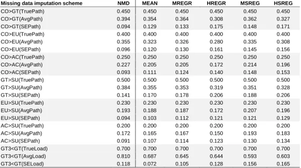
Table A1a. Monte Carlo experiment results with a sample size of 100 and 30% missing data.
Missing data imputation scheme NMD MEAN MREGR HREGR MSREG HSREG
CO>GT(TruePath) 0.450 0.450 0.450 0.450 0.450 0.450 CO>GT(AvgPath) 0.394 0.354 0.364 0.308 0.362 0.327 CO>GT(SEPath) 0.094 0.129 0.133 0.175 0.148 0.171 CO>EU(TruePath) 0.400 0.400 0.400 0.400 0.400 0.400 CO>EU(AvgPath) 0.355 0.323 0.326 0.280 0.335 0.308 CO>EU(SEPath) 0.096 0.120 0.130 0.161 0.145 0.156 CO>AC(TruePath) 0.250 0.250 0.250 0.250 0.250 0.250 CO>AC(AvgPath) 0.227 0.205 0.205 0.172 0.214 0.196 CO>AC(SEPath) 0.093 0.111 0.124 0.140 0.148 0.153 GT>SU(TruePath) 0.500 0.500 0.500 0.500 0.500 0.500 GT>SU(AvgPath) 0.384 0.355 0.353 0.319 0.351 0.328 GT>SU(SEPath) 0.141 0.170 0.178 0.206 0.188 0.206 EU>SU(TruePath) 0.230 0.230 0.230 0.230 0.230 0.230 EU>SU(AvgPath) 0.193 0.188 0.187 0.172 0.207 0.196 EU>SU(SEPath) 0.094 0.103 0.112 0.121 0.121 0.129 AC>SU(TruePath) 0.200 0.200 0.200 0.200 0.200 0.200 AC>SU(AvgPath) 0.172 0.165 0.167 0.150 0.193 0.183 AC>SU(SEPath) 0.091 0.107 0.114 0.123 0.130 0.134 GT3<GT(TrueLoad) 0.700 0.700 0.700 0.700 0.700 0.700 GT3<GT(AvgLoad) 0.810 0.687 0.645 0.644 0.593 0.603 GT3<GT(SELoad) 0.118 0.072 0.105 0.128 0.156 0.165
Table A1b. Monte Carlo experiment results with a sample size of 100 and 40% missing data.
Missing data imputation scheme NMD MEAN MREGR HREGR MSREG HSREG
CO>GT(TruePath) 0.450 0.450 0.450 0.450 0.450 0.450 CO>GT(AvgPath) 0.394 0.309 0.315 0.247 0.307 0.264 CO>GT(SEPath) 0.094 0.188 0.193 0.240 0.223 0.251 CO>EU(TruePath) 0.400 0.400 0.400 0.400 0.400 0.400 CO>EU(AvgPath) 0.355 0.280 0.283 0.225 0.275 0.240 CO>EU(SEPath) 0.096 0.185 0.194 0.226 0.219 0.239 CO>AC(TruePath) 0.250 0.250 0.250 0.250 0.250 0.250 CO>AC(AvgPath) 0.227 0.186 0.182 0.145 0.189 0.165 CO>AC(SEPath) 0.093 0.170 0.188 0.185 0.208 0.211 GT>SU(TruePath) 0.500 0.500 0.500 0.500 0.500 0.500 GT>SU(AvgPath) 0.384 0.320 0.324 0.272 0.311 0.280 GT>SU(SEPath) 0.141 0.222 0.227 0.263 0.246 0.270 EU>SU(TruePath) 0.230 0.230 0.230 0.230 0.230 0.230 EU>SU(AvgPath) 0.193 0.191 0.189 0.163 0.189 0.178 EU>SU(SEPath) 0.094 0.144 0.157 0.163 0.186 0.195 AC>SU(TruePath) 0.200 0.200 0.200 0.200 0.200 0.200 AC>SU(AvgPath) 0.172 0.177 0.177 0.146 0.186 0.164 AC>SU(SEPath) 0.091 0.157 0.172 0.170 0.204 0.208 GT3<GT(TrueLoad) 0.700 0.700 0.700 0.700 0.700 0.700 GT3<GT(AvgLoad) 0.810 0.479 0.440 0.444 0.395 0.398 GT3<GT(SELoad) 0.118 0.261 0.295 0.306 0.347 0.359
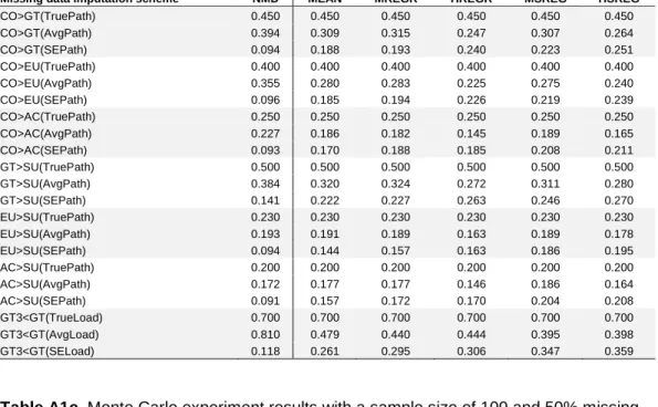
Table A1c. Monte Carlo experiment results with a sample size of 100 and 50% missing data.
Missing data imputation scheme NMD MEAN MREGR HREGR MSREG HSREG
CO>GT(TruePath) 0.450 0.450 0.450 0.450 0.450 0.450 CO>GT(AvgPath) 0.394 0.241 0.248 0.170 0.227 0.183 CO>GT(SEPath) 0.094 0.272 0.287 0.327 0.323 0.345 CO>EU(TruePath) 0.400 0.400 0.400 0.400 0.400 0.400 CO>EU(AvgPath) 0.355 0.215 0.211 0.145 0.190 0.159 CO>EU(SEPath) 0.096 0.263 0.284 0.308 0.323 0.327 CO>AC(TruePath) 0.250 0.250 0.250 0.250 0.250 0.250 CO>AC(AvgPath) 0.227 0.146 0.151 0.110 0.136 0.113 CO>AC(SEPath) 0.093 0.227 0.242 0.228 0.276 0.270 GT>SU(TruePath) 0.500 0.500 0.500 0.500 0.500 0.500 GT>SU(AvgPath) 0.384 0.267 0.263 0.208 0.238 0.207 GT>SU(SEPath) 0.141 0.292 0.303 0.337 0.351 0.359 EU>SU(TruePath) 0.230 0.230 0.230 0.230 0.230 0.230 EU>SU(AvgPath) 0.193 0.172 0.168 0.137 0.163 0.139 EU>SU(SEPath) 0.094 0.212 0.239 0.213 0.264 0.259 AC>SU(TruePath) 0.200 0.200 0.200 0.200 0.200 0.200 AC>SU(AvgPath) 0.172 0.152 0.149 0.118 0.153 0.135 AC>SU(SEPath) 0.091 0.219 0.242 0.213 0.270 0.263 GT3<GT(TrueLoad) 0.700 0.700 0.700 0.700 0.700 0.700 GT3<GT(AvgLoad) 0.810 0.284 0.250 0.263 0.217 0.214 GT3<GT(SELoad) 0.118 0.451 0.480 0.483 0.511 0.526
Table A2a. Monte Carlo experiment results with a sample size of 300 and 30% missing data.
Missing data imputation scheme NMD MEAN MREGR HREGR MSREG HSREG
CO>GT(TruePath) 0.450 0.450 0.450 0.450 0.450 0.450 CO>GT(AvgPath) 0.390 0.348 0.354 0.300 0.367 0.333 CO>GT(SEPath) 0.075 0.113 0.113 0.162 0.110 0.138 CO>EU(TruePath) 0.400 0.400 0.400 0.400 0.400 0.400 CO>EU(AvgPath) 0.349 0.312 0.313 0.262 0.321 0.289 CO>EU(SEPath) 0.069 0.101 0.106 0.151 0.108 0.133 CO>AC(TruePath) 0.250 0.250 0.250 0.250 0.250 0.250 CO>AC(AvgPath) 0.219 0.198 0.195 0.161 0.206 0.188 CO>AC(SEPath) 0.062 0.078 0.083 0.108 0.090 0.100 GT>SU(TruePath) 0.500 0.500 0.500 0.500 0.500 0.500 GT>SU(AvgPath) 0.381 0.357 0.352 0.312 0.359 0.334 GT>SU(SEPath) 0.127 0.152 0.158 0.195 0.156 0.179 EU>SU(TruePath) 0.230 0.230 0.230 0.230 0.230 0.230 EU>SU(AvgPath) 0.192 0.183 0.178 0.163 0.199 0.188 EU>SU(SEPath) 0.062 0.072 0.078 0.089 0.077 0.082 AC>SU(TruePath) 0.200 0.200 0.200 0.200 0.200 0.200 AC>SU(AvgPath) 0.165 0.157 0.154 0.141 0.176 0.166 AC>SU(SEPath) 0.058 0.067 0.072 0.081 0.073 0.077 GT3<GT(TrueLoad) 0.700 0.700 0.700 0.700 0.700 0.700 GT3<GT(AvgLoad) 0.811 0.691 0.649 0.652 0.606 0.623 GT3<GT(SELoad) 0.113 0.042 0.076 0.090 0.120 0.115
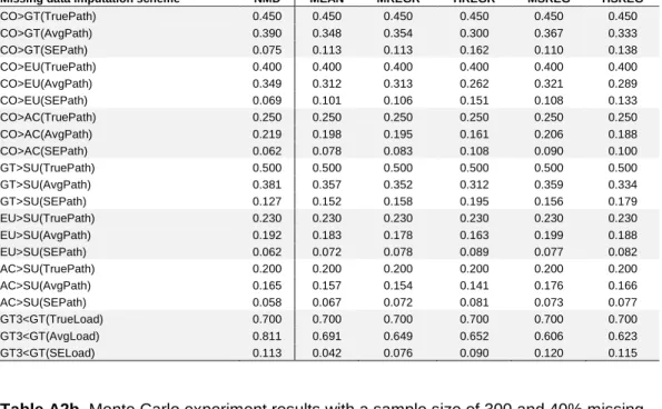
Table A2b. Monte Carlo experiment results with a sample size of 300 and 40% missing data.
Missing data imputation scheme NMD MEAN MREGR HREGR MSREG HSREG
CO>GT(TruePath) 0.450 0.450 0.450 0.450 0.450 0.450 CO>GT(AvgPath) 0.390 0.309 0.311 0.240 0.308 0.264 CO>GT(SEPath) 0.075 0.160 0.165 0.224 0.173 0.209 CO>EU(TruePath) 0.400 0.400 0.400 0.400 0.400 0.400 CO>EU(AvgPath) 0.349 0.273 0.274 0.211 0.271 0.234 CO>EU(SEPath) 0.069 0.147 0.152 0.204 0.162 0.191 CO>AC(TruePath) 0.250 0.250 0.250 0.250 0.250 0.250 CO>AC(AvgPath) 0.219 0.176 0.174 0.132 0.178 0.156 CO>AC(SEPath) 0.062 0.113 0.116 0.142 0.129 0.138 GT>SU(TruePath) 0.500 0.500 0.500 0.500 0.500 0.500 GT>SU(AvgPath) 0.381 0.323 0.320 0.264 0.314 0.282 GT>SU(SEPath) 0.127 0.191 0.196 0.246 0.207 0.235 EU>SU(TruePath) 0.230 0.230 0.230 0.230 0.230 0.230 EU>SU(AvgPath) 0.192 0.186 0.180 0.157 0.201 0.184 EU>SU(SEPath) 0.062 0.087 0.094 0.101 0.096 0.099 AC>SU(TruePath) 0.200 0.200 0.200 0.200 0.200 0.200 AC>SU(AvgPath) 0.165 0.161 0.161 0.138 0.180 0.163 AC>SU(SEPath) 0.058 0.083 0.085 0.097 0.099 0.103 GT3<GT(TrueLoad) 0.700 0.700 0.700 0.700 0.700 0.700 GT3<GT(AvgLoad) 0.811 0.496 0.461 0.475 0.423 0.440 GT3<GT(SELoad) 0.113 0.221 0.256 0.253 0.296 0.286
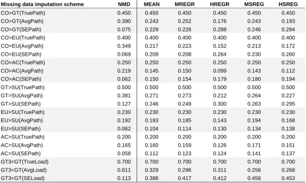
Table A2c. Monte Carlo experiment results with a sample size of 300 and 50% missing data.
Missing data imputation scheme NMD MEAN MREGR HREGR MSREG HSREG
CO>GT(TruePath) 0.450 0.450 0.450 0.450 0.450 0.450 CO>GT(AvgPath) 0.390 0.243 0.252 0.176 0.243 0.193 CO>GT(SEPath) 0.075 0.229 0.226 0.288 0.246 0.284 CO>EU(TruePath) 0.400 0.400 0.400 0.400 0.400 0.400 CO>EU(AvgPath) 0.349 0.217 0.223 0.152 0.213 0.172 CO>EU(SEPath) 0.069 0.209 0.208 0.264 0.230 0.260 CO>AC(TruePath) 0.250 0.250 0.250 0.250 0.250 0.250 CO>AC(AvgPath) 0.219 0.145 0.150 0.099 0.143 0.112 CO>AC(SEPath) 0.062 0.150 0.154 0.179 0.180 0.194 GT>SU(TruePath) 0.500 0.500 0.500 0.500 0.500 0.500 GT>SU(AvgPath) 0.381 0.271 0.273 0.212 0.264 0.227 GT>SU(SEPath) 0.127 0.246 0.249 0.300 0.263 0.295 EU>SU(TruePath) 0.230 0.230 0.230 0.230 0.230 0.230 EU>SU(AvgPath) 0.192 0.183 0.185 0.143 0.194 0.168 EU>SU(SEPath) 0.062 0.104 0.114 0.130 0.134 0.138 AC>SU(TruePath) 0.200 0.200 0.200 0.200 0.200 0.200 AC>SU(AvgPath) 0.165 0.160 0.159 0.126 0.171 0.151 AC>SU(SEPath) 0.058 0.112 0.123 0.124 0.141 0.137 GT3<GT(TrueLoad) 0.700 0.700 0.700 0.700 0.700 0.700 GT3<GT(AvgLoad) 0.811 0.329 0.296 0.311 0.256 0.268 GT3<GT(SELoad) 0.113 0.386 0.417 0.412 0.456 0.453
Table A3a. Monte Carlo experiment results with a sample size of 500 and 30% missing data.
Missing data imputation scheme NMD MEAN MREGR HREGR MSREG HSREG
CO>GT(TruePath) 0.450 0.450 0.450 0.450 0.450 0.450 CO>GT(AvgPath) 0.389 0.346 0.352 0.296 0.363 0.328 CO>GT(SEPath) 0.070 0.110 0.109 0.162 0.104 0.135 CO>EU(TruePath) 0.400 0.400 0.400 0.400 0.400 0.400 CO>EU(AvgPath) 0.343 0.308 0.309 0.258 0.317 0.286 CO>EU(SEPath) 0.067 0.100 0.102 0.149 0.102 0.129 CO>AC(TruePath) 0.250 0.250 0.250 0.250 0.250 0.250 CO>AC(AvgPath) 0.219 0.197 0.192 0.159 0.204 0.183 CO>AC(SEPath) 0.052 0.070 0.077 0.103 0.077 0.090 GT>SU(TruePath) 0.500 0.500 0.500 0.500 0.500 0.500 GT>SU(AvgPath) 0.380 0.354 0.348 0.309 0.358 0.333 GT>SU(SEPath) 0.124 0.151 0.157 0.196 0.151 0.175 EU>SU(TruePath) 0.230 0.230 0.230 0.230 0.230 0.230 EU>SU(AvgPath) 0.189 0.180 0.176 0.160 0.198 0.184 EU>SU(SEPath) 0.055 0.064 0.070 0.083 0.065 0.073 AC>SU(TruePath) 0.200 0.200 0.200 0.200 0.200 0.200 AC>SU(AvgPath) 0.164 0.154 0.151 0.137 0.174 0.164 AC>SU(SEPath) 0.054 0.063 0.067 0.077 0.061 0.067 GT3<GT(TrueLoad) 0.700 0.700 0.700 0.700 0.700 0.700
Table A3b. Monte Carlo experiment results with a sample size of 500 and 40% missing data.
Missing data imputation scheme NMD MEAN MREGR HREGR MSREG HSREG
CO>GT(TruePath) 0.450 0.450 0.450 0.450 0.450 0.450 CO>GT(AvgPath) 0.389 0.307 0.308 0.236 0.307 0.265 CO>GT(SEPath) 0.070 0.155 0.158 0.223 0.164 0.201 CO>EU(TruePath) 0.400 0.400 0.400 0.400 0.400 0.400 CO>EU(AvgPath) 0.343 0.270 0.267 0.205 0.267 0.230 CO>EU(SEPath) 0.067 0.145 0.151 0.205 0.157 0.188 CO>AC(TruePath) 0.250 0.250 0.250 0.250 0.250 0.250 CO>AC(AvgPath) 0.219 0.174 0.171 0.129 0.175 0.151 CO>AC(SEPath) 0.052 0.098 0.104 0.135 0.109 0.125 GT>SU(TruePath) 0.500 0.500 0.500 0.500 0.500 0.500 GT>SU(AvgPath) 0.380 0.321 0.315 0.260 0.312 0.280 GT>SU(SEPath) 0.124 0.187 0.194 0.246 0.200 0.230 EU>SU(TruePath) 0.230 0.230 0.230 0.230 0.230 0.230 EU>SU(AvgPath) 0.189 0.181 0.178 0.152 0.194 0.177 EU>SU(SEPath) 0.055 0.078 0.082 0.097 0.084 0.090 AC>SU(TruePath) 0.200 0.200 0.200 0.200 0.200 0.200 AC>SU(AvgPath) 0.164 0.161 0.157 0.134 0.178 0.163 AC>SU(SEPath) 0.054 0.072 0.076 0.088 0.078 0.082 GT3<GT(TrueLoad) 0.700 0.700 0.700 0.700 0.700 0.700 GT3<GT(AvgLoad) 0.811 0.501 0.468 0.486 0.433 0.455 GT3<GT(SELoad) 0.113 0.213 0.245 0.237 0.281 0.267
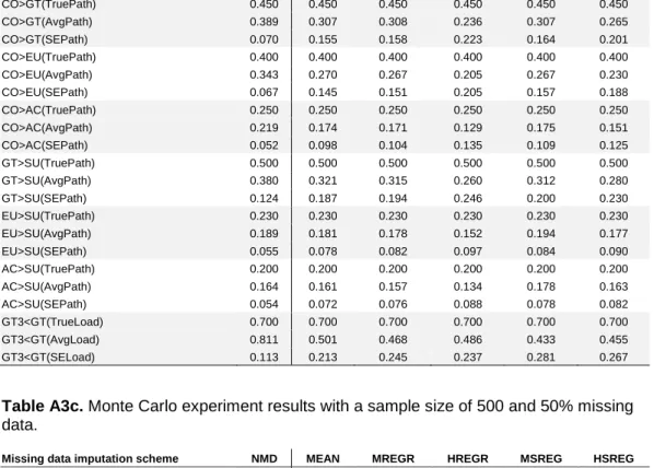
Table A3c. Monte Carlo experiment results with a sample size of 500 and 50% missing data.
Missing data imputation scheme NMD MEAN MREGR HREGR MSREG HSREG
CO>GT(TruePath) 0.450 0.450 0.450 0.450 0.450 0.450 CO>GT(AvgPath) 0.389 0.245 0.250 0.171 0.238 0.193 CO>GT(SEPath) 0.070 0.218 0.218 0.288 0.236 0.274 CO>EU(TruePath) 0.400 0.400 0.400 0.400 0.400 0.400 CO>EU(AvgPath) 0.343 0.213 0.216 0.150 0.209 0.168 CO>EU(SEPath) 0.067 0.205 0.206 0.260 0.218 0.251 CO>AC(TruePath) 0.250 0.250 0.250 0.250 0.250 0.250 CO>AC(AvgPath) 0.219 0.143 0.144 0.098 0.140 0.113 CO>AC(SEPath) 0.052 0.133 0.137 0.168 0.154 0.168 GT>SU(TruePath) 0.500 0.500 0.500 0.500 0.500 0.500 GT>SU(AvgPath) 0.380 0.270 0.270 0.206 0.263 0.227 GT>SU(SEPath) 0.124 0.240 0.243 0.301 0.254 0.285 EU>SU(TruePath) 0.230 0.230 0.230 0.230 0.230 0.230 EU>SU(AvgPath) 0.189 0.172 0.170 0.134 0.183 0.158 EU>SU(SEPath) 0.055 0.098 0.103 0.119 0.105 0.115 AC>SU(TruePath) 0.200 0.200 0.200 0.200 0.200 0.200 AC>SU(AvgPath) 0.164 0.157 0.158 0.127 0.175 0.151 AC>SU(SEPath) 0.054 0.090 0.095 0.103 0.104 0.109 GT3<GT(TrueLoad) 0.700 0.700 0.700 0.700 0.700 0.700 GT3<GT(AvgLoad) 0.811 0.339 0.307 0.322 0.267 0.285 GT3<GT(SELoad) 0.113 0.373 0.403 0.395 0.443 0.431
Appendix B: Business Process Modeling Approaches Used
The figure below illustrates the two types of representations used in the business process redesign projects. In the context of our data analyses example, the one on the left was coded as 1, and the one on the right as 0. They correspond to high and low communication flow orientations, respectively, of the business process modeling approach used.Figure A1. High (left) and low (right) communication flow orientations of the business process modeling approach.
Appendix C: Questionnaire Used in Empirical Study
The question-statements below were used for latent variable measurement in the illustrative study. Except for communication flow orientation (C1), all
question-statements were answered on 7-point Likert-type scales.
Communication flow orientation (C1)
• C11: Coded as either 1 or 0, corresponding to high or low
communication flow orientation of the business process modeling approach used.
Usefulness in the development of IT solutions (C2)
• C21: This process modeling approach is useful in the development of
a generic IT solution to automate the redesigned process.
• C22: Creating a generic IT solution to enable the redesigned process
is easy based on this process modeling approach.
• C23: Graphical process representations using this approach facilitate
the generation of a generic IT solution to automate the redesigned process.
Ease of understanding (C3)
• C31: Processes modeled using this approach are easy to understand.
• C32: Graphical representations of processes using this approach are
clear.
• C33: This process modeling approach leads to graphical models that
are easy to understand.
Accuracy (C4)
• C41: This process modeling approach leads to accurate process
representations.
• C42: Models created using this approach are correct representations
of a process.
• C43: Graphical representations using this approach clearly reflect the
Impact on redesign success (C5)
• C51: Using this process modeling approach is likely to contribute to
the success of a process redesign project.
• C52: Success chances are improved if this process modeling approach
is used.
• C53: Using the graphical process representations in this approach is