Interruptional Activity and Simulation of Transposable Elements

(1)

Interruptional Activity and Simulation of

Transposable Elements

A Thesis Submitted to the

College of Graduate and Postdoctoral Studies

in Partial Fulfillment of the Requirements

for the degree of Doctor of Philosophy

in the Department of Computer Science

University of Saskatchewan

Saskatoon

By

Lingling Jin

c

(2)

Permission to Use

In presenting this thesis in partial fulfilment of the requirements for a Postgraduate degree from the University

of Saskatchewan, I agree that the Libraries of this University may make it freely available for inspection.

I further agree that permission for copying of this thesis in any manner, in whole or in part, for scholarly

purposes may be granted by the professor or professors who supervised my thesis work or, in their absence,

by the Head of the Department or the Dean of the College in which my thesis work was done. It is understood

that any copying or publication or use of this thesis or parts thereof for financial gain shall not be allowed without my written permission. It is also understood that due recognition shall be given to me and to the

University of Saskatchewan in any scholarly use which may be made of any material in my thesis.

Requests for permission to copy or to make other use of material in this thesis in whole or part should be

addressed to:

Head of the Department of Computer Science

176 Thorvaldson Building 110 Science Place University of Saskatchewan Saskatoon, Saskatchewan Canada S7N 5C9

(3)

Abstract

Transposable elements (TEs) are interspersed DNA sequences that can move or copy to new positions within

a genome. The active TEs along with the remnants of many transposition events over millions of years

constitute 46.69% of the human genome. TEs are believed to promote speciation and their activities play a

significant role in human disease. The 22AluY and 6AluS TE subfamilies have been the most active TEs in recent human history, whose transposition has been implicated in several inherited human diseases and

in various forms of cancer by integrating into genes. Therefore, understanding the transposition activities is very important.

Recently, there has been some work done to quantify the activity levels of active Alu transposable elements based on variation in the sequence. Here, given this activity data, an analysis of TE activity based on the

position of mutations is conducted. Two different methods/simulations are created to computationally predict so-called harmful mutation regions in the consensus sequence of a TE; that is, mutations that occur in these

regions decrease the transposition activities dramatically. The methods are applied to AluY, the youngest and most active Alu subfamily, to identify the harmful regions laying in its consensus, and verifications are presented using the activity of AluY elements and the secondary structure of the AluYa5 RNA, providing evidence that the method is successfully identifying harmful mutation regions. A supplementary simulation

also shows that the identified harmful regions covering theAluYa5 RNA functional regions are not occurring by chance. Therefore, mutations within the harmful regions alter the mobile activity levels of active AluY

elements. One of the methods is then applied to two additional TE families: theAlu family andL1 family, in detecting the harmful regions in these elements computationally.

Understanding and predicting the evolution of these TEs is of interest in understanding their powerful

evolutionary force in shaping their host genomes. In this thesis, a formal model of TE fragments and their

interruptions is devised that provides definitions that are compatible with biological nomenclature, while still

providing a suitable formal foundation for computational analysis. Essentially, this model is used for fixing

terminology that was misleading in the literature, and it helps to describe further TE problems in a precise way. Indeed, later chapters include two other models built on top of this model: the sequential interruption

model and the recursive interruption model, both used to analyze their activity throughout evolution.

The sequential interruption model is defined between TEs that occur in a genomic sequence to estimate how

often TEs interrupt other TEs, which has been shown to be useful in predicting their ages and their activity

throughout evolution. Here, this prediction from the sequential interruptions is shown to be closely related to a classic matrix optimization problem: the Linear Ordering Problem (LOP). By applying a well-studied

(4)

TEs in the human genome is predicted from a single genome. A comparison of the TE ordering between

Tabu search and the method used in [47] shows that Tabu search solves the TE problem exceedingly more

efficiently, while it still achieves a more accurate result. As a result of the improved efficiency, a prediction

on all human TEs is constructed, whereas it was previously only predicted for a minority fraction of the set of the human TEs.

When many insertions occurred throughout the evolution of a genomic sequence, the interruptions nest in

a recursive pattern. The nested TEs are very helpful in revealing the age of the TEs, but cannot be fully

represented by the sequential interruption model. In the recursive interruption model, a specific

context-free grammar is defined, describing a general and simple way to capture the recursive nature in which TEs nest themselves into other TEs. Then, each production of the context-free grammar is associated with a

probability to convert the context-free grammar into a stochastic context-free grammar that maximizes the

applications of the productions corresponding to TE interruptions. A modified version of an algorithm to

parse context-free grammars, the CYK algorithm, that takes into account these probabilities is then used to

find the most likely parse tree(s) predicting the TE nesting in an efficient fashion.

The recursive interruption model produces small parse trees representing local TE interruptions in a genome.

These parse trees are a natural way of grouping TE fragments in a genomic sequence together to form

interruptions. Next, some tree adjustment operations are given to simplify these parse trees and obtain more

standard evolutionary trees. Then an overall TE-interaction network is created by merging these standard

evolutionary trees into a weighted directed graph. This TE-interaction network is a rich representation of the

predicted interactions between all TEs throughout evolution and is a powerful tool to predict the insertion

evolution of these TEs. It is applied to the human genome, but can be easily applied to other genomes.

Furthermore, it can also be applied to multiple related genomes where common TEs exist in order to study

the interactions between TEs and the genomes.

Lastly, a simulation of TE transpositions throughout evolution is developed. This is especially helpful in

understanding the dynamics of how TEs evolve and impact their host genomes. Also, it is used as a verification

technique for the previous theoretical models in the thesis. By feeding the simulated TE remnants and activity

data into the theoretical models, a relative age order is predicted using the sequential interruption model, and a quantified correlation between this predicted order and the input age order in the simulation can be

calculated. Then, a TE-interaction network is constructed using the recursive interruption model on the

simulated data, which can also be converted into a linear age order by feeding the adjacency matrix of the

network to Tabu search. Another correlation is calculated between the predicted age order from the recursive

interruption model and the input age order. An average correlation of ten simulations is calculated for each

model, which suggests that in general, the recursive interruption model performs better than the sequential

interruption model in predicting a correct relative age order of TEs. Indeed, the recursive interruption model

(5)

Acknowledgements

First and foremost, I would like to express my sincere gratitude to Dr. Ian McQuillan, my Master’s and

Ph.D. supervisor, for his incredible amount of guidance and support in overcoming numerous difficulties that

I have faced through my research.

Special thanks to Dr. Longhai Li, my cognate committee member, who has provided me with lots of ideas

and guidance on statistical aspects of my thesis.

I am also grateful to the other members of my advisory committee: Dr. Tony Kusalik, Dr. Mark Keil, and

Dr. Michael Domaratzki for their invaluable suggestions and comments.

I want to acknowledge my colleagues in the Bioinformatics lab and my friends for their friendship and helpful

discussions.

I am grateful to my husband, Shi, and my children, April and Avery, for being the love and happiness of my

life. Very special thanks goes to my husband for helping me with the implementation and graphic design in

the thesis.

Last but not the least, I would like to acknowledge my parents, Xin and Zhimei, and my parents-in-law,

(6)

List of Tables

1.1 Human diseases caused by TE insertions. . . 4

2.1 A summary of the percentage of TE content in the human genome. . . 13

2.2 Overview of different classes of transposable elements (reflecting the classification in Figure 2.4) in the human genome. . . 14

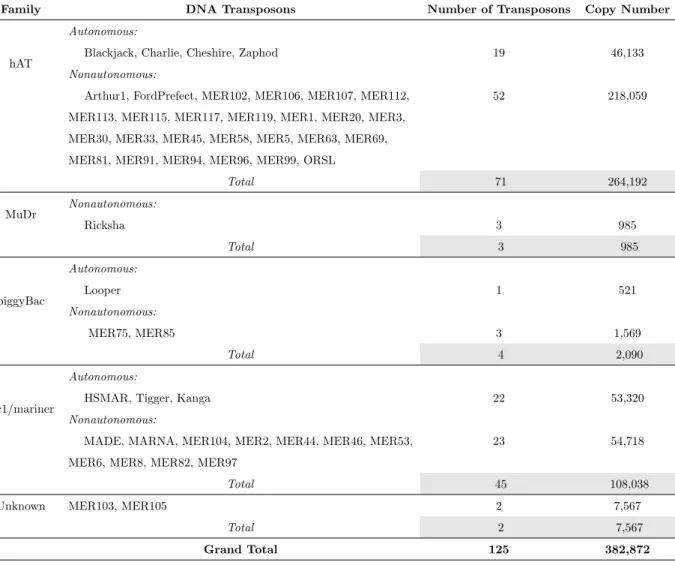
2.3 A summary of currently recognizable DNA transposons in the human genome. . . 16

2.4 An example of a tabular summary of RepeatMasker. . . 21

3.1 Simulated and observed correlations between mutations and mobile activities. . . 40

3.2 The harmful mutation regions inAluY elements. . . 42

3.3 The percentage of mutations. . . 43

3.4 Comparison types of the group comparison analysis. . . 47

3.5 The matrix of observed and simulated ratios in each window. . . 49

3.6 Identified harmful windows withλ= 0.05. . . 51

3.7 Identified harmful regions with the start and end positions of each region. . . 51

3.8 The percentage of mutations grouped by bins. . . 52

3.9 The harmful mutation regions inAlu elements. . . 56

3.10 Comparison between the harmful mutation regions inAluY andAlu elements. . . 57

3.11 The harmful mutation regions inL1 elements. . . 59

4.1 A table of two TE fragments on the human chromosome 1. . . 65

4.2 A summary of the total number of TE fragments in the human genome. . . 67

4.3 A table of six TE fragments on the human chromosome 1. . . 68

5.1 An example of an interruption. . . 73

5.2 An example of distances between three TE fragments . . . 74

5.3 A summary of the total number of sequential interruptions detected in the human genome. . 75

5.4 An example of sequential interruptions on chromosome 1. . . 76

5.5 The outlier TEs in Figure 5.3 . . . 87

6.1 An example of recursive interruptions on the X chromosome. . . 88

6.2 A summary of the order-pruned sequences of the transposon regions on the Y chromosome. . 98

6.3 A summary of the order-pruned sequence in the human genome. . . 99

6.4 An example of three atomic patterns of interruptions. . . 101

6.5 List of TE names along with known information. . . 107

6.6 The order-pruned sequences only containingχs. . . 108

6.7 The age order of TEs in the TE-interaction network in Figure 6.13. . . 112

6.8 Comparison between the age orders of TEs in Figure 6.13. . . 113

6.9 List of TE names along with their information. . . 115

7.1 Parameters of the simulation . . . 124

7.2 The input age order, activation time, deactivation time and lifespans of TEs in the simulation. 130 7.3 The relative age order calculated by Tabu search from IM. . . 133

7.4 The indegree and outdegree of each node in the network. . . 137

7.5 The relative age order calculated by Tabu search from AM. . . 138

(9)

List of Figures

2.1 Repeated DNA sequences in eukaryotic genomes, adapted from [119]. Transposons are marked

in red. . . 8

2.2 The proportions of TEs in several genomes. . . 9

2.3 Conceptual diagrams representing the transposition mechanisms. . . 10

2.4 The classification of transposable elements can be represented as a tree. . . 11

2.5 Structural features of the DNA transposons. . . 15

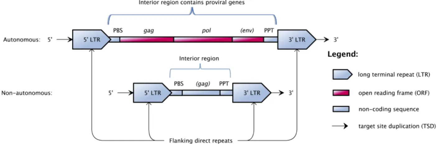
2.6 Structural features of the LTR retrotransposons. . . 17

2.7 Structural features of the LTR retrotransposons. . . 18

2.8 The resultant relative age order of 360 TEs calculated in [47], where the numbers on the left axis represent positions in the age order. . . 28

3.1 Structure ofAluelements. . . 31

3.2 The plot of the 52AluY elements from [12] . . . 34

3.3 The heat map of the number of mutations ofAluY elements. . . 36

3.4 The Pearson’s coefficients of correlation ofAluY elements. . . 38

3.5 The flow chart of the algorithm in Section 3.4.2. . . 39

3.6 The distribution of correlations. . . 41

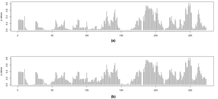
3.7 Thep-values andq-values of theAluY elements. . . 42

3.8 The secondary structure of anAluYa5 RNA. . . 44

3.9 The distribution of coverage. . . 46

3.10 Observed ratiosRi of the six comparison types in Table 3.4. . . 48

3.11 The empirical distribution of simulated ratios of the windoww20. . . 50

3.12 The secondary structure of anAluY RNA. . . 53

3.13 The distribution of the coverage of random generated regions. . . 54

3.14 The heat map of the number of mutations of theAlu elements. . . 55

3.15 The Pearson’s coefficients of correlation of theAlu elements. . . 55

3.16 Thep-values andq-values of theAlu elements. . . 56

3.17 The Pearson’s coefficients of correlation of theL1 elements. . . 58

3.18 Thep-values andq-values of theL1 elements. . . 60

4.1 A conceptual visualization of TE fragments. . . 66

4.2 A conceptual visualization of a genomic sequence. . . 69

5.2 A conceptual diagram of the permuted interruptional matrix. . . 82

5.3 A comparison between two orderings. . . 86

6.2 A parse tree showing the derivation of 01010. . . 91

6.3 A diagram showing an insertion. . . 92

6.4 A parse tree of G from Definition 21 that yields ¯so. . . 93

6.5 The most likely parse tree of G from Definition 21 that yields ¯so. . . 96

6.7 The two most-likely trees of the same order-pruned sequence. . . 100

6.8 The corresponding parse trees in Table 6.4. . . 102

6.9 An example of condensing a tree. . . 103

6.10 An example of converting a parse tree to an evolutionary tree . . . 104

6.11 An example of converting an interruption tree to an evolutionary tree. . . 104

6.12 Another example of converting an interruption tree to an evolutionary tree. . . 105

(10)

6.14 The directed graph generated by merging the interruption trees. . . 116

7.1 A workflow of simulated data verifying the theoretical models in previous chapters. . . 132 7.2 A comparison between the input age order and the predicted age order calculated by Tabu

search from the simulated IM. . . 134 7.3 The TE-interaction network calculated from the recursive interruption model on the simulated

data. . . 135 7.4 A comparison between the input age order and the predicted age order calculated by Tabu

(11)

List of Abbreviations

TE Transposable Elements bp base pairs Kbp Kilobase pairs Mbp Megabase pairs RU Repbase Update RM RepeatMasker

Myr Million years MYA Million Years Ago

LINE Long Interspersed Nuclear Elements SINE Short Interspersed Nuclear Elements LTR Long Terminal Repeat

TIR Terminal Inverted Repeat TSD Target Site Duplication

ORF Open Reading Frame

IM Interruption Matrix LOP Linear Ordering Problem CFG Context-free Grammar

SCFG Stochastic Context-free Grammar

(12)

Chapter 1

Introduction and objectives

Transposable elements were first discovered by Barbara McClintock in the 1950s during her studies of maize, work for which McClintock received the Nobel Prize in Physiology or Medicine in 1983. The patterns of

colour in maize kernels changed in different breeding crosses, which was interpreted in her study as a result

of the regulation of gene activity by some mobile genetic elements. These elements can move from place

to place within/between the chromosomes. As the elements move, they mutate genes in some of the cells

and change the colour of maize kernels due to their effects on pigmentation genes [14]. These mobile genetic

elements are named transposable elements (TEs), ortransposons.

Transposable elements were dismissed at one point as being useless, but they are emerging to be thought

of as major players in evolution. Indeed, the impact of TEs on genome evolution appears to be extensive

and they are even believed to promote speciation [42] and can therefore be seen as a driver of evolution.

The evolutionary history of a TE family in a species may represent a plentiful source of information about

genome evolution. Additionally, more and more evidence is emerging that active TEs play a significant role

in human biology and disease as they create genetic diversity in human populations and can integrate into

genes, potentially causing disease. However, little analysis is currently being undertaken in determining what

factors influence their activity, what occurred throughout evolution, and in understanding how TEs change

over time.

1.1

Motivations

In this section, the motivations of the thesis will be discussed from the impacts of TEs on genomes as well

(13)

1.1.1

The impact of TEs on genomes

Though the number of genes in a genome grows from bacteria to higher organisms, it is the repeats, especially

TEs, that account for the major differences in genome size within species, and even between closely related

species [14]; that is, genome size is not correlated with the complexity of the organism [143]. Retrotransposons

are major players in promoting the increase of genome size. It has been shown using genomic studies of ancient

human remains that the human genome is continuing to expand at a rate between 1 and 10 million base pairs per million years, and this expansion is heavily influenced by retrotransposition, the transposition of retrotransposons [71]. For example, there are ∼2,000 L1 and∼7,000Alu copies accumulated over the past

∼6 Myr of human evolution [127]. Not only in humans, TEs influence plant genome sizes significantly as well. The sizes of plant genomes span across many orders of magnitude ranging from about 63 Mbp of theGenlisea

genome [51] to more than 110,000 Mbp of the lilyFritillaria assyriaca[4], which is primarily the consequence of polyploidization and TE proliferation [27]. Moreover, studies of maize [122] and the riceOryza australiensis

[116] show that LTR retrotransposition doubled the genome size in the two species independently.

TEs also impact host genomes by generating genomic instability due to their continuous activity over years.

The major way that a retrotransposon alters genome function is by inserting itself into protein-coding or

regulatory regions. There are a number of examples of genetic disorders that are caused by the expansion of

microsatellites [65, 26, 28], and non-LTR retrotransposons are the source of microsatellites. For example, it

is known that about 20% of all microsatellites shared by the human and chimpanzee genomes lie withinAlu

elements [72].

Retrotransposons can generate genomic rearrangements as well, such as deletions, duplications, inversions,

or translocations. It was observed in cultured human cells that ∼20% of L1 insertions were related with structural rearrangements [30], including insertion-mediated deletions; that is, concurrent deletions at the

insertion site. It has been estimated that during primate evolution, about 45,000 insertion-mediated deletions

might have removed over 30 Mbp of genomic sequence [29].

Moreover, transposons can mediate the formation of a new gene family [106] or impact gene expression.

TEs may influence the expression of surrounding genes often due to a regulatory promoter1_{and terminator}2

sequence occuring in LTRs [101]. Thus, TEs can be used as tools in genetic research to either open or

terminate the expression of nearby genes.

Last but not least, TEs are of interest for their own sake as they have been a powerful evolutionary force in

shaping genomes. The ubiquity of TEs raises a number of questions about the relationships between TEs

1_A_promoter_{is a region of DNA that facilitates the transcription of a particular gene. Promoters are located near the genes}

they regulate, on the same strand and typically upstream (towards the 5’ region of the sense strand).

(14)

and their host genomes and the significance of these elements on the evolution of their hosts. Knowledge

of the location of TEs can also be helpful in the determination of the evolutionary history of a locus of a

genome.

1.1.2

Transposable elements causing human diseases

TEs have co-existed with their host organisms for an exceptionally long period, during which their

transpo-sition activities have contributed to their host genomes in both positive and negative ways. Transpotranspo-sition

of currently active elements as well as recombination involving repetitive sequences can be responsible for

genetic diseases, and there is a growing understanding of the specific negative impacts of TEs in human

dis-ease. Generally, the TE-associated insertional mutagenesis and recombination may cause DNA damage and

contribute to human diseases. In this subsection, some examples of human diseases caused by TE activities will be described.

Retrotransposition events occur in both the germline and somatic tissues [30]. The transposition of TEs has

been implicated in processes ranging from cancer to brain development. The brain has one of the highest

average frequencies of transposable element activity of all tissues in the human body [86]. In very recent

research on Alzheimer’s disease, a molecular mechanism of the Alzheimer’s process was proposed to be caused

byAluelements losing their normal controls as a person ages, wreaking havoc on the machinery that supplies energy to brain cells and leading to a loss of neurons and dementia [86]. The authors hypothesize that through human-specific neurologic pathways,Aluinsertions in mitochondrial genes can cause progressive neurological disfunction, which may underlie the origin of higher cognitive function [86]. Therefore, retrotransposons have

played an important role in primate evolution.

Human TEs have been reported to cause several types of cancer, such as breast cancer, colon cancer,

retinoblastoma, neurofibromatosis, hepatoma, etc., through insertional mutagenesis of genes that are

im-portant to malignant transformation [10]. For example, the most up-to-date research in [126] has shown that a hotL1 (defined as showing at least one-third of the activity ofL1RP in [17]) source TE on Chromosome 17 of a patient’s genome interrupted somatic repression in normal colon tissues, and initiated colorectal cancer

by disrupting the APC tumor suppressor gene [103]. The fact thatL1 transpositions occur in human tumors suggests the possibility that somatic L1 insertions may play a role as driver mutations during the stages of initiation, progression, and metastasis of tumors [126].

Non-LTR retrotransposons are deemed as the major source of TE-related mutagenesis in the human genome.

There have been a number of cases shown to cause heritable diseases, as a result of human genetic disorders caused by de novo L1, Alu and SVA insertions, such as haemophilia, cystic fibrosis, Apert syndrome, neu-rofibromatosis, Duchenne muscular dystrophy, β-thalassaemia, and hypercholesterolaemia [30]. Table 1.1,

(15)

TE insertion Chromosome Disease caused by TE insertion Reported papers Aluinsertions X Hemophilia B [34, 25] X Hemophilia A [25] X Dent’s disease [25] X X-linked agammaglobulinemia [25] X X-linked severe combined immunodeficiency [34] X Glycerol kinase deficiency [34] X Adrenoleukodystrophy [25]

X Menkes disease [52]

X Hyper-immunoglobulin M syndrome [5]

1 Retinal blinding [25]

1 Type 1 antithrombin deficiency [25] 2 Muckle-Wells syndrome [25] 2 Hereditary non-polyposis colorectal cancer [25] 3 Hypocalciuric hypercalcemia and hyperparathyroidism [34] 3 Cholinesterase deficiency [34] 3 Aplasia anterior pituitary [25] 5 Associated with leukemia [34] 5 Hereditary desmoid disease [34] 7 Chronic hemolytic anemia [95]

7 Cystic fibrosis [24]

8 Branchio-oto-renal syndrome [25] 8 Lipoprotein lipase deficiency [110]

8 CHARGE syndrome [142]

9 Walker Warburg syndrome [15] 10 Autoimmune lymphoproliferative syndrome [25]

10 Apert syndrome [34]

11 Complement deficiency [34] 11 Acute intermittent porphyria [25] 12 Human-specific evolutionary change [15] 12 Mucolipidosis type II

13 and 17 Breast cancer [34] 17 Neurofibromatosis [34]

L1insertions

X Choroideremia [25]

X Chronic granulomatous disease [25] X X-linked Duchenne muscular dystrophy [25, 111]

X Hemophilia A [25]

X Hemophilia B [25]

X X-linked retinitus pigmentosa [25] X Coffin-Lowry syndrome [25]

5 Colon cancer [25]

9 Fukuyama-type congenital muscular dystrophy [25]

11 Beta-thalassemia [25]

11 Pyruvate dehydrogenase complex deficiency [15]

(16)

adapted from [9], gives more details about some diseases caused by the insertions ofL1 andAlu, the active elements in humans.

1.1.3

Perspective

It is important to understand the patterns of the activities of TEs and the factors that may change their

activities, because such TE activities can powerfully influence the structure of the genome, including the

capacity of chromosomes to rearrange and to regulate transcription. And, as discussed above, they are often

important in understanding human disease. Further, identifying repetitive DNA sequences in eukaryotic DNA

is essential in genome analysis, because these repeats offer an opportunity to study molecular evolution as

“molecular fossils” in evolutionary studies based on comparative analysis of genomes from different species. It

is amazing how much regarding evolution can be inferred from a single genome sequence, as most evolutionary

analysis require sequences from multiple genomes. This might be useful in situations where TEs change quickly and multiple genomes are not available. The dynamic of what causes TE families as a whole to

evolve is also of interest.

1.2

Objectives and layout of the thesis

The research of this thesis will be conducted only on data regarding human TEs. We intend to contribute

to the understanding of how the TE propagation through evolution shapes the genome, how the age and

lifespan of TEs can be predicted from a single genome, and a determination of certain factors that affect the

activities of active TEs that may cause human disease. The major work of the thesis will be composed of

four major goals with their corresponding chapters:

Goal 1 Create a model that describes TEs and remnants of TEs formally (Chapter 4).

After an extensive literature survey on transposable elements, we found that there did not exist a

standard model that describes/defines the topic in a clear and consistent way. For example, the use of

many terms are frequently ambiguous, such as a transposable element, a subfamily of a transposon, a

clade of transposons, a group of transposable element fragments, etc. Moreover, some computational

approaches regarding TEs were described in a prose-like language, without any formal algorithms, which

brought in different ambiguities when reproducing the method. Therefore, our first goal is to create

a formal model that consists of an initial definition of TEs, TE fragments, and interruptions between

TEs, etc. This model does not attempt to capture the molecular operations of TE movement, but only describes the order and distance between TE fragments in genomic sequences by grouping homologous

(17)

as a baseline in describing our other formal models.

Goal 2 Understand the factors that affect the activities of active TEs, and understand how activity is affected

(Chapter 3).

The factors that change transpositional activities is largely a mystery, and it might be the result of a

number of factors or combinations of them. Our goal is to understand what factors affect a transposon’s

activity level, and determine how they affect them. We will study “harmful mutation regions” in active

TEs, where mutations within these regions will decrease the activities of the host element.

Goal 3 Predict the age, lifespan, and activity of TEs in the human genome from the remnants of these elements

from a genome. In order to make this prediction, two formal models are created in Chapters 5 and 6

that describe and can be used to analyze and predict the ages of TEs.

By analyzing TE remnants in genomic sequences, the knowledge of TE activities can be inferred. Then

understanding how TEs interrupted within each other will reveal information regarding the age and

lifespan of a transposon; that is, when TEs activated and deactivated through evolution. Then the

dynamics of TE transpositions through evolution can be predicted. This goal can be achieved by two

sub-goals as follows.

• Understand interruption activities between TEs.

The interruptions are classified into two different types based on the fashion in which they nested.

The formal model inGoal 1is applied to these two models. The first application was the

Sequen-tial Interruption model, which captures the interruptions between pairs of TEs, and structures the

abundance of these interruptions into a so-called interruption matrix. The second application was

the Recursive Interruption model that describes the nested nature of the recursive interruptions

with a context-free grammar. The parse trees of the grammar can illustrate the relationships of

TE nesting using the structure of the trees.

• Predict an overall TE-interaction network.

Several of the small interruption trees can be combined together to form a weighted directed graph

to illustrate all TE activity, which can also help in the understanding of TE evolution as a whole.

Such a graph is created for all TEs in order and is used to predict the age order and lifespans of

these TEs.

Goal 4 Understand the dynamics of TEs transpositions through evolution (Chapter 7).

Another goal of the thesis is to create a simulation that imitates the evolutionary history of the

(18)

relative positions in the genome are comparable to the actual TE remnants in the human genome. Then

by analyzing the generated TE remnants and predicting the TE evolution using the tools generated

forGoal 3, this work can be used as a type of verification of the models and algorithms in Goal 3.

A simulation also allows for specific hypotheses regarding TEs to be tested, which is of interest to the community. Moreover, some aspects of Goal 2 inform the simulation itself. The two sub-goals are

listed as follows.

• Simulate TE propagation through evolution.

• Use the simulated interruptions to verify the prediction models. Hence, the various goals of this thesis are quite interconnected:

• Goal 1is used as a basic frame work forGoal 3andGoal 4;

• Goal 2andGoal 3inform the process of simulation ofGoal 4;

• Goal 4is used as a verification forGoal 3.

These goals all help in the study of transposable elements, their influence on genomes, and their ability to

(19)

Chapter 2

Background

Transposable elements are one type of repetitive DNA sequences in eukaryotic genomes. Typically, repetitive

DNA sequences are broadly classified into two large families within eukaryotic genomes, tandem repeats and

dispersed repeats, and each of these two families can be further divided into several subfamilies as shown in

Figure 2.1.

Figure 2.1: Repeated DNA sequences in eukaryotic genomes, adapted from [119]. Transposons are marked in red.

TEs are found in both eukaryotic and prokaryotic organisms, including plants, animals, bacteria, and archaea.

As shown in Figure 2.2 (summarized from [14, 125, 148, 136]), the proportion of TEs in a genome differs

broadly depending on the organism, ranging from a few percent (0.3%) in the bacteria Escherichia coli to almost the entire genome (>80%) in maize Zea mays. In humans, 66–69% of the genome is repetitive or repeat-derived [32], whereas coding sequences comprise less than 5% of the genome. The majority of repeats

in human are transposable elements, making up about 45% of the genome [88].

(20)

Figure 2.2: The proportions of TEs in several genomes. As shown in the stacked bars, the TE proportions in yeast and fruitfly are shown as value ranges (3% to 5% in yeast, and 15% to 22% in fruitfly). The reason that there exists ranges is because the transposons in these species are transient components of those genomes, which means the repeat fraction of these genomes evolves very rapidly within species [100].

diversified into forms that share very little sequence homology. Over time, inactivated copies of these elements

have accumulated and now comprise a significant proportion of many genomes, serving as an important opportunity to study molecular evolution. This is because every element in the genome represents a “fossil

record” that throughout evolution accumulates mutations randomly and independently, meaning that they

can be used to study genomic changes both between and within species. “The mammalian genome could be

compared, somewhat poetically, with a coral reef, in which the transposable elements are the coral, the reef

is built of the fossils of their ancestors, and the genes are the inhabiting fish, anemones, sea stars, and so

on.” [130]

So far in this chapter, a brief introduction about TEs including their proportions in genomes and some

key terminologies has been provided, which gives a general idea about what TEs are. In the next sections, some necessary knowledge regarding the topic of the thesis will be provided from the perspectives of biology,

(21)

2.1

Biological background

2.1.1

Classification of transposable elements

Transposition is defined as the movement of genetic material from one genomic location, the donor site, to another, thetarget site, within the same genome [50]. Transposable elements are traditionally classified into two broad classes on the basis of their transposition mechanism and sequence organization [43]:

Figure 2.3: Conceptual diagrams representing the transposition mechanisms. (a) Retrotransposons (“copy-and-paste” mechanism) copy themselves in two stages: first from DNA to RNA by transcription, then from RNA back to DNA by reverse transcription. The DNA copy is then inserted into the genome in a new position. (b) DNA transposons (“cut-and-paste” mechanism) do not involve an RNA intermediate. The transpositions in these classes are catalyzed by various types of transposase enzymes.

• Class I elements (“copy-and-paste” mechanism as the conceptual diagrams shown in Figure 2.3 (a)) are those that transpose via reverse transcription of an RNA intermediate, referred to asretrotransposons. The RNA intermediate is first transcribed from a genomic copy of DNA, then reverse-transcribed into

DNA that is identical to the original DNA by a reverse transcriptase1 encoded in the TE sequence,

(22)

and each complete replication cycle produces one new copy into the host DNA [145]. Consequently,

retrotransposons can increase the copy numbers of elements and thereby increase genome size; indeed,

they are major players in promoting the increase of genome size.

• Class II elements (“cut-and-paste” mechanism as the conceptual diagrams shown in Figure 2.3 (b)) move primarily through a DNA-mediated mechanism of excision and insertion, and are often called

DNA transposons.

The class I and class II elements coexist in an extensive range of eukaryotes, which suggests their ancient

evolutionary origins; however, there exist many variations in the activity, copy number, and diversity of TEs

in the genomes of different species [49].

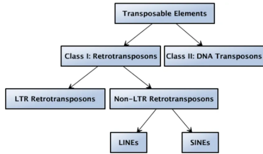
TEs can also be divided into several types on the basis of the structural features of their sequences: LTR

retrotransposons, LINEs, SINEs, and DNA transposons (summarized as in Figure 2.4). Note that this

classification is according to structural features of TEs as in Section 2.1.2, which is equivalent to the simplified

classification shown in the red subtree in Figure 2.1. Among the four types of TEs, non-LTR retrotransposons

(LINEs and SINEs) have been major factors of genome evolution by providing diversity and plasticity to the

genome [71].

Figure 2.4: The classification of transposable elements can be represented as a tree.

TEs are also described as beingautonomous ornon-autonomous based on whether or not they encode their own genes for transposition. Those transposable elements that possess a complete set of transposition protein

domains are calledautonomous. Transposable elements that lack an intact set of mobility-associated genes are called non-autonomous TEs. The transposition of non-autonomous TEs requires involvement of protein(s) from either autonomous element(s) or from the genome in which they reside. For example, the autonomous

Acelements in maize can transpose themselves regardless of the other TEs present in the genome ; in contrast, the non-autonomousDselements cannot transpose without the aids of one or more copies ofAcelements in the genome [50].

(23)

Nevertheless, the term autonomous does not indicate that a TE is active or functional. A TE is defined as ac-tiveif it can transpose either autonomously or non-autonomously. Typically, the lifespan of one transposable element starts from an activation of the transposon, followed by a burst of transpositions, while accumulating

mutations, followed by the slowing of mobile activity after additional mutations. The transposon then ebbs further until it becomes inactive. The inactive elements, referred to as fossil transposable elements, become relics and can get interrupted by the transpositions of other active elements [47]. Active elements comprise

only a tiny proportion of the TE content of the genomes of most organisms. The genomes of eukaryotes

are filled with thousands of copies of the remnants of inactive TEs. For example, there are roughly 50,000

autonomous and 200,000 non-autonomous fossil DNA transposons in the human genome, and none of them

are active any more [50].

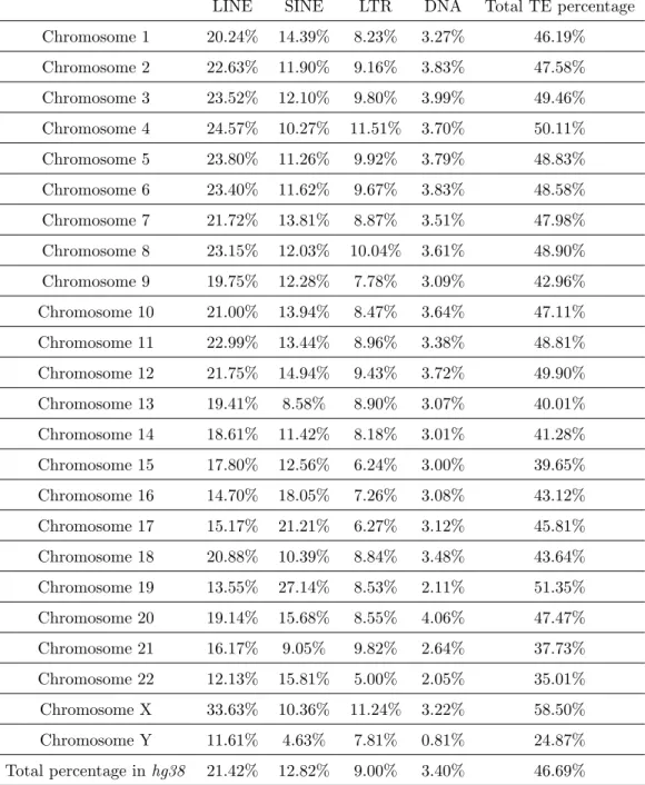
The human genome consists of a large amount of TEs and their remnants. Table 2.1 lists the percentage of

TE contents in each chromosome calculated from the hg38 assembly2 _{of the human genome. It should be}

noted that the total percentage of TEs we calculated onhg38 is 46.69% in the thesis, which is slightly higher than the 45% estimated in the year of 2009 [88] from a previous version of the human genome.

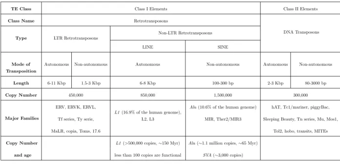
Within each type, TEs can be even further subdivided into families then subfamilies, based on their details

of the transposition mechanism, and sequence similarity. For example, L1, L2 are families under LINEs, while Alu, SVA are families under SINEs; furthermore, there are subfamiliesAluY, AluJ, AluS under the family of Alu. Table 2.2 (information from [84]) is a detailed summary of each type of TE in the human genome.

A gust of transposition of L1 and Alu elements in the primate lineage occurred about 40 million years ago (MYA), followed by a slowing of transpositional activity since then [73]. Recent evidence indicates that there are 35 to 40 subfamilies ofAlu,SVA, andL1 elements staying actively mobile in the human genome [104, 71], and all of the active transposable elements only comprise less than 0.05% of the nucleotides in the human

genome. It has been estimated that active human transposons generate about one insertion for every 10 to

100 live births [69, 89, 31]. The rate ofL1 retrotransposition is estimated as 1/140 live births per generation [38], and one newAlu insertion is generated for every 20 live human births [31]. The active TEs along with their copy numbers are listed in Table 2.2 as well.

2.1.2

Structural features of TE sequences

In mammals, almost all transposable elements fall into one of the four types listed in Figure 2.4, of which

three transpose through RNA intermediates and one transposes directly as DNA. Transposable elements use

different strategies for their evolutionary survival (summarized from [84]):

(24)

LINE SINE LTR DNA Total TE percentage Chromosome 1 20.24% 14.39% 8.23% 3.27% 46.19% Chromosome 2 22.63% 11.90% 9.16% 3.83% 47.58% Chromosome 3 23.52% 12.10% 9.80% 3.99% 49.46% Chromosome 4 24.57% 10.27% 11.51% 3.70% 50.11% Chromosome 5 23.80% 11.26% 9.92% 3.79% 48.83% Chromosome 6 23.40% 11.62% 9.67% 3.83% 48.58% Chromosome 7 21.72% 13.81% 8.87% 3.51% 47.98% Chromosome 8 23.15% 12.03% 10.04% 3.61% 48.90% Chromosome 9 19.75% 12.28% 7.78% 3.09% 42.96% Chromosome 10 21.00% 13.94% 8.47% 3.64% 47.11% Chromosome 11 22.99% 13.44% 8.96% 3.38% 48.81% Chromosome 12 21.75% 14.94% 9.43% 3.72% 49.90% Chromosome 13 19.41% 8.58% 8.90% 3.07% 40.01% Chromosome 14 18.61% 11.42% 8.18% 3.01% 41.28% Chromosome 15 17.80% 12.56% 6.24% 3.00% 39.65% Chromosome 16 14.70% 18.05% 7.26% 3.08% 43.12% Chromosome 17 15.17% 21.21% 6.27% 3.12% 45.81% Chromosome 18 20.88% 10.39% 8.84% 3.48% 43.64% Chromosome 19 13.55% 27.14% 8.53% 2.11% 51.35% Chromosome 20 19.14% 15.68% 8.55% 4.06% 47.47% Chromosome 21 16.17% 9.05% 9.82% 2.64% 37.73% Chromosome 22 12.13% 15.81% 5.00% 2.05% 35.01% Chromosome X 33.63% 10.36% 11.24% 3.22% 58.50% Chromosome Y 11.61% 4.63% 7.81% 0.81% 24.87% Total percentage inhg38 21.42% 12.82% 9.00% 3.40% 46.69%

Table 2.1: A summary of the percentage of TE content in the human genome (calculated onhg38). It also lists the percentage of TEs of four different types and summarized by chromosomes.

(25)

TE Class Class I Elements Class II Elements

Class Name Retrotransposons

DNA Transposons Type LTR Retrotransposons

Non-LTR Retrotransposons

LINE SINE

Mode of Autonomous Non-autonomous Autonomous Non-autonomous Autonomous Non-autonomous Transposition

Length 6-11 Kbp 1.5-3 Kbp 6-8 Kbp 100-300 bp 2-3 Kbp 80-3000 bp

Copy Number 450,000 850,000 1,500,000 300,000

Major Families

ERV, ERVK, ERVL,

L1(16.9% of the human genome),

Alu(10.6% of the human genome) hAT, Tc1/mariner, piggyBac, Tf series, Ty serie, L2, L3 MIR, Ther2/MIR3 Sleeping Beauty, Tn series, Mu, Mos1,

MaLR, copia, Toms, 17.6 Tol2, hobo, transits, MITEs

Copy Number L1(>500,000 copies,∼150 Myr) Alu(∼1.1 million copies,∼65 Myr) and age less than 100 copies are functional SVA(∼3,000 copies)

Table 2.2: Overview of different classes of transposable elements (reflecting the classification in Figure 2.4) in the human genome.

• LINEs and SINEs depend on vertical transmission, meaning that the new “offspring” TEs are produced from their “parent” TEs within the host genome.

• DNA transposons depend on horizontal transfer, meaning that the transfer between members of the same species are not in a parent-child relationship.

• LTR retrotransposons use both strategies.

It should be noted that it is beneficial to discuss the biological details in order to gain an understanding of the variation, since different parts of this thesis deal with different specific TEs and TE properties. Also, different

existing TE-related tools take into account specific features, which are worth discussing. The biological

insights of each type of TE is summarized as follows (information from [41], [84], [121], and [71]):

DNA transposons

DNA transposons are prevalent in bacteria, but are also found in the genomes of many metazoa, including

insects, worms, and humans [70]. These elements are generally excised from one genomic site and integrated

into another by a “cut-and-paste” mechanism (Figure 2.3).

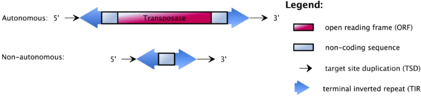
As shown in Figure 2.5, DNA transposons are usually composed of terminal inverted repeat sequences (TIRs;

in Figure 2.5, big blue arrows are in opposite directions) at their front and rear ends. Between TIRs is one

ORF3 _{sequence (red boxes in Figure 2.5, 2.6, and 2.7) that encodes a transposase protein that recognizes}

(26)

Figure 2.5: Structural features of DNA transposons, which may contain both autonomous and non-autonomous elements.

the TIRs and cuts the transposon out of its genomic site. The two ends of the transposon are then held

together by the transposase while it finds another site in the DNA to cut and insert into. Thus, the process

uses a so-called “cut-and-paste” mechanism. All DNA transposons, both autonomous and non-autonomous,

are surrounded by short duplications of the genomic sequence at their insertion sites, called target site duplications (TSDs)4. This occurs because the double-stranded target site is cut in a staggered manner, the single-stranded flanks are then repaired, and two repeats in the same orientation (called direct repeats, opposite to inverted repeats), are created on both sides of the integrated TE [50]. The TSDs can either be

of fixed or variable lengths, depending on the type of elements. In fact, the integration of almost all TEs

results in the target-site duplications as shown in black thin arrows flanking the element in Figure 2.5, 2.6,

and 2.7. In fact, non-autonomous DNA transposons are usually derived from an autonomous transposon by

an internal deletion.

There are nearly no known active DNA transposons in mammals (except bats5) [71]. It has been previously believed that DNA transposons have not been active in the mammalian lineage for at least 40 million years (Mys). There are only 15 superfamilies to which currently known eukaryotic DNA transposons belong

(de-spite their enormous diversity and abundance): hapaev, En/Spm (CACTA), hAT, Harbinger (Pif ), ISL2EU (IS4EU), Kolobok, Mariner, Merlin, Mirage, MuDR(MULE), Novosib, P, PiggyBac, Rehavkus,andTransib

[68].

The human genome contains the remnants of at least five major families of DNA transposons, which can be

subdivided into many transposons with independent origins. Table 2.3, derived from [112], is a summary of

currently recognizable DNA transposons in the human genome with copy number greater than 100.

DNA transposons generally transpose to genomic sites less than 100 Kbp from their original site, called

RNA that signals a termination of translation) in a given reading frame.

4_{When a transposon inserts itself into host DNA, a short (7-20bp) segment of host DNA is replicated at the site of insertion,}

which is called‘target site duplication’ or TSD.

5_{Eight different families of DNA transposons, including hAT family members and piggyBac-like elements, were found active}

(27)

Family DNA Transposons Number of Transposons Copy Number

hAT

Autonomous:

Blackjack, Charlie, Cheshire, Zaphod 19 46,133

Nonautonomous:

Arthur1, FordPrefect, MER102, MER106, MER107, MER112, MER113, MER115, MER117, MER119, MER1, MER20, MER3, MER30, MER33, MER45, MER58, MER5, MER63, MER69, MER81, MER91, MER94, MER96, MER99, ORSL

52 218,059 Total 71 264,192 MuDr Nonautonomous: Ricksha 3 985 Total 3 985 piggyBac Autonomous: Looper 1 521 Nonautonomous: MER75, MER85 3 1,569 Total 4 2,090 Tc1/mariner Autonomous:

HSMAR, Tigger, Kanga 22 53,320

Nonautonomous:

MADE, MARNA, MER104, MER2, MER44, MER46, MER53, MER6, MER8, MER82, MER97

23 54,718

Total 45 108,038

Unknown MER103, MER105 2 7,567

Total 2 7,567

Grand Total 125 382,872

Table 2.3: A summary of currently recognizable DNA transposons in the human genome with copy number greater than 100.

“local hopping” [70] (e.g., the Drosophila P element), and some are able to make distant “hops” (e.g., the fish Tc1/mariner element) as well. Moreover, DNA transposons are inclined to have short lifespans within a species compared to LINEs, and why DNA transposons have lost their ability to move for millions of years

of mammalian evolution requires further studies.

Retrotransposons

Retrotransposons are very different from DNA transposons. They replicate and mobilize through an RNA

intermediate via a “copy-and-paste” mechanism involving the enzyme reverse transcriptase and an endonu-clease.

Retrotransposons typically can be divided into long terminal repeat (LTR) retrotransposons (Figure 2.6) and

(28)

nuclear elements (LINEs) and short interspersed nuclear elements (SINEs). Most of retrotransposons are

no longer able to retrotranspose. Retrotransposons have taken over large portions of the genomes of most

plants and animals. In plants, most are LTR-retrotransposons , while in mammals non-LTR retrotransposons

predominate.

Some retrotransposons are site-specific (only insert at specific sites in the genome). For instance, the

non-LTR retrotransposons of the R1 and R2 families insert themselves only at specific sequences within the ribosomal RNA genes of insects [71]. In contrast, there are some non-LTR retrotransposons of theL1 family that insert at many different sites that are AT-rich (e.g., 5’-TTTT/AA-3’, where “/” signifies the cut site)

[71].

LTR Retrotransposons. The LTR retrotransposons have many characteristics akin to retroviruses. They

are called LTR retrotransposons because they have long terminal repeat (LTR) sequences of 300 to 1000

nucleotides at their two ends in direct orientation. These direct repeats have the same sequence in the same

order, e.g., ABCD. In contrast, inverted repeats in DNA transposons are ABCD at one end and DCBA at

the other (example from [70]). The LTRs contain promoters that stimulate transcription of the RNA of

the element. Figure 2.6 shows the structural features of both the autonomous and non-autonomous LTR

retrotransposons. Autonomous LTR retrotransposons have the products required for transposition encoded in

open reading frames (ORFs), while non-autonomous LTR retrotransposons lack most or all coding sequence for transposition, and their internal region can be variable in length and unrelated to the autonomous

elements.

Figure 2.6: Structural features of the autonomous and non-autonomous LTR retrotransposons (the genes in parentheses are optional).

According to [68], there are 6 superfamilies in LTR retrotransposons: Copia, Gypsy, BEL, ERV1, ERV2, and ERV3. Among a variety of LTR retrotransposons, only the vertebrate-specifc endogenous retroviruses (ERVs) appear to have been active in the mammalian genome. Most (85%) of the LTR

(29)

retrotransposon-derived TE remnants consist only of an isolated LTR, where the internal sequence has been lost by homologous

recombination [102].

Non-LTR Retrotransposons. Non-LTR retrotransposons are quite different from LTR-retrotransposons

in their mode of regulation, replication, and structure. They are divided into autonomous elements (LINEs)

and non-autonomous elements (SINEs). As shown in Figure 2.7, non-LTR retrotransposons have an internal promoter at their 5’ end (pol II for LINEs andpol III for SINEs) that is important for starting expression or transcription of the element RNA. Non-LTR Retrotransposons end by a simple sequence repeat at their

3’ end, usually a poly(A) tail (a region containing many A nucleotides in a row). All LINEs described so far usually encode two proteins necessary for their retrotransposition. The 3’ tail of some SINEs and the 3’

tail of LINEs present in the same genome are related to each other (share homology) [41], which indicates

that SINEs must be aided by the transposition machinery of partner LINEs in the process of transposition

[35].

Figure 2.7: Structural features of the non-LTR retrotransposons, that contain autonomous LINEs and non-autonomous SINEs.

In humans, LINEs are about 6 Kbplong, harbouring an internalpolymerase II promoter and encoding two open reading frames (ORFs3). ORF 1 encodes a nucleic acid binding protein (nabp) with chaperone6 and esterase7activities, and ORF 2 encodes apolprotein with reverse transcriptase1and endonuclease8activities. It is believed that the LINE machinery is responsible for most reverse transcription in the genome, that also

includes the transposition of the non-autonomous SINEs. Three distantly related LINE families are found in

the human genome: L1,L2, and L3, among which, onlyL1 is still active.

The non-autonomousAlus are thought to use the transposition machinery of LINEs. They are about 100−

300 bp with no terminal repeats, harbour an internal polymerase III promoter and encode no proteins. The human genome contains a few families of SINEs: the active Alu, SVA, and the inactive MIR and

6_{In molecular biology,}_{molecular chaperones}_{are proteins that assist the non-covalent folding or unfolding and the assembly}

or disassembly of other macromolecular structures, but do not occur in these structures when the structures are performing their normal biological functions, having completed the processes of folding and/or assembly.

7_An_esterase_{is a hydrolase enzyme that splits esters into an acid and an alcohol in a chemical reaction with water called}

hydrolysis.

(30)

Ther2/MIR3.

One of the key facts about human retrotransposons is that humans have active TEs, called L1s (the only active family in LINEs in humans), and these active TEs make an endonuclease and a reverse transcriptase

that drives the retrotransposition of themselves and of other TEs, calledAluandSVA(the active families in SINEs in humans).

2.2

Bioinformatics background

2.2.1

Sequence alignment

Many biological structures can be naturally represented by strings/sequences, such as DNA, RNA, and

proteins. Sequence alignment is a method for biological sequence comparison, which can reveal similarity between different sequences. There exist a number of sequence alignment methods/tools, and some of them

are based on dynamic programming alignment algorithms, such as the Needleman-Wunsch algorithm [109] or

the Smith-Waterman algorithm [133], which compute the optimal alignments between two sequences.

A multiple sequence alignment (MSA), a natural extension of two-sequence comparisons, is a sequence

align-ment of three or more sequences. MSAs are a powerful way to study biological sequences. In a MSA, similar

characters among a set of sequences are aligned together in columns. Often, the goal with aligning sequences

is to reveal homology, which indicates similar position, structure, function, or characteristics due to evolu-tionary relatedness [57]. Sequences can be aligned to visualize the effect of evolution across the whole family.

Ideally, a column of aligned characters all diverge from a common ancestor. The resulting MSA can infer

se-quence homology and guide phylogenetic analysis to assess the sese-quences’ shared evolutionary origins. From

this, aconsensus sequence can be calculated from the result of a MSA. The consensus sequence of a multiple alignment is, informally, a “best” single sequence to represent the alignment. For example, a consensus for

three DNA sequences

A C A G T A G

A C− −T C G A G− −G C G

isACAGT CG. Notice that it is possible to have more than one consensus.

It is computationally expensive to calculate the optimal alignment between multiple sequences, therefore,

(31)

2.2.2

Repbase Update — the database of repetitive sequences

Most eukaryotic repetitive sequences have been reconstructed into a database called Repbase Update (RU)

[63], a database of the consensus sequences of repetitive elements (not only TEs, but also other repeats),

that are present in diverse eukaryotic organisms. RU is the major reference database of repetitive sequences

used in DNA annotation and analysis. Each sequence in the database is accompanied by a short descrip-tion and references to the original contributors. It has been developed by Dr. Jerzy Jurka since 1990. It

continues to grow through its community-driven annotation and submission tools and now is widely used

in genome sequencing projects worldwide as a reference collection for masking and annotation of repetitive

DNA. Consequently, the repeat classification based on RU is used in many other databases (such as UCSC

genome database [120], Ensembl annotation [2]) and in secondary databases of repetitive elements. Some

TE discovery and annotation tools also use RU as their reference library, such as the ones discussed in

Section 2.2.3.

2.2.3

TE discovery tools

According to [13], there are usually two major goals in identifying TEs in genomic sequences:

• mask them as a preprocessing step in some bioinformatic tasks, such as gene finding;

• study them directly to make inferences about the biology or evolution of TEs.

These aims are incorporated into the most common systems used to detect individual instances of TEs in

genome sequences.

The detection of TEs can be conducted in different ways, depending on the level of knowledge about the

repeats that are taken into account when detecting them in a genome sequence. As suggested in [13], [121],

[88], and [91], the approaches can be classified into four categories as follows.

• Library-based approaches search the repetitive sequences by comparing input data to a set of reference sequences (known TEs) contained in a library.

• Signature-based approaches search TEs using knowledge from their known structures.

• Comparative-genomics approaches use the fact that transposition creates large insertions that can be detected in multiple sequence alignments and rely on neither library nor structural features.

• De novo approaches look for similar subsequences found at multiple positions within a sequence.

(32)

Library-based techniques

Library-based methods identify repetitive sequences by comparing input datasets against a set of reference

repeat sequences (known TEs) [121]. The library can either be user-defined, or it can be a general library,

such as the commonly used Repbase Update [63]. The advantages of library-based techniques are that this

method is usually efficient and effective at finding repeats in the library, whereas the disadvantages are that

it heavily depends on how much we already know, and fails to detect the repeats that do not exist in the

library.

The most widely used library-based program is RepeatMasker [131], which is the major library-based tool

used in repeat identification. It has been identified as one of the most accurate tools in detecting TEs

and it has become a standard tool for finding repeats in genomes [91]. Using precompiled repeat libraries,

RepeatMasker finds copies of known repeat families represented in Repbase Update. As the name implies, it

was designed to discover repeats and mask them. The program performs a similarity search based on local

alignments, then outputs masked genomic DNA and a tabular summary of TE content.

Table 2.4 is an example of the tabular summary output by RepeatMasker, which shows eight repeat fragments

identified in a query sequence named HSU08988, and each row represents one fragment. The columns are information about each fragment. For example, the first fragment in the list is from position 6563 to position

6781 in the query sequence. It is a fragment from position 103 to position 336 of the complementary

sequence of elementMER7A (belongs to a DNA transposonMER2 family), with 15.6% percent divergence, 6.2% deletion, and 0% insertion compared to theMER7Aconsensus in the Repbase Update.

position in query position in repeat

score % % % query C matching repeat left end begin

div. del. ins. sequence begin end left + repeat class/family begin end left 1306 15.6 6.2 0 HSU08988 6563 6781 -22462 C MER7A DNA/MER2 0 336 103 12204 10 2.4 1.8 HSU08988 6782 7714 -21529 C TIGGER1 DNA/MER2 0 2418 1493

279 3 0 0 HSU08988 7719 7751 -21492 + (TTTTA)n Simple repeat 1 33 0 1765 13.4 6.5 1.8 HSU08988 7752 8022 -21221 C AluSx SINE/Alu -23 289 1 12204 10 2.4 1.8 HSU08988 8023 8694 -20549 C TIGGER1 DNA/MER2 -925 1493 827

1984 11.1 0.3 0.7 HSU08988 8695 9000 -20243 C AluSg SINE/Alu -5 305 1 12204 10 2.4 1.8 HSU08988 9001 9695 -19548 C TIGGER1 DNA/MER2 -1591 827 2 711 21.2 1.4 0 HSU08988 9696 9816 -19427 C MER7A DNA/MER2 -224 122 2

Table 2.4: An example of a tabular output of RepeatMasker. In the tabular summary, there are eight repeat fragments listed, which were identified in the query sequence named HSU08988. Each row represents one fragment, and the columns are the detailed information about the fragments.

RepeatMasker uses multi-processor systems and a simple database search approach (e.g., BLAST [78]),

(33)

in the field of TE identification, in the thesis, TE fragments are defined with the aid of RepeatMasker in

Chapter 4.

In addition to the tabular output as in Table 2.4, there are several library-based repeat detection tools

that use visualization to display the repeat fragments, such as CENSOR [64]. It applies the same kind of

approach used in RepeatMasker, then graphically maps detected repeats with colour-coding of different types

of repeats.

Signature-based techniques

Unlike library-based tools, all signature-based tools employ prior knowledge about the common structural

features shared by different TEs in the same class as introduced in Section 2.1.2, and it is less biased by

similarity to the set of known elements. Given a particular repeat group, signature-based repeat detection

tools search query sequences for motifs9 _{and spatial arrangements characteristic of that group [121]. This}

approach can be used to find new elements of known groups, but not new groups of elements. The limitation

of such approaches is that it depends entirely on how much is known about the structure of elements belonging

to particular groups, and also on the existence of characteristic structures.

LTR retrotransposons are bordered by long terminal repeats (LTRs), with a more detailed structure shown in Figure 2.7. Based on the structure, there have been several tools developed to detect solely LTR

retro-transposons, by searching for the common structural signals existing in LTR retrotransposons as listed below.

Some of the features correspond to parameters that can be adjusted by the users of these tools, such as:

• a range of lengths of the LTR sequences;

• the distance between the two LTRs of an element;

• the presence of TSDs4_{at each end;}

• the presence of critical regions for replication, such as the primer binding site (PBSs)10 and the poly-purine tract (PPTs);

• the percent identity between the two LTRs;

• the existence of some conserved motifs corresponding to the genes they encode.

9_{A sequence}_motif_{means a sequence pattern of nucleotides in a DNA sequence or amino acids in a protein.}

10_A_{primer binding site} _{is a region of a nucleotide sequence where an RNA or DNA single-stranded primer binds to start}

replication. The primer binding site is on one of the two complementary strands of a double-stranded nucleotide polymer, in the strand which is to be copied, or is within a single-stranded nucleotide polymer sequence.

(34)

For example, the method LTR STRUC [98] searches a query sequence for pairs of similar LTRs separated

by a distance expected for this group of retrotransposons. The pairwise alignment of LTRs is then used to

calculate the boundaries of the LTRs on the original segment, which should span a full-length element from

the start of the 5’ LTR to the end of the 3’ LTR. LTR par [66] is a similar structure-based method to detect LTR retrotransposons, which improves on some of the weaknesses in LTR STRUC. Both LTR-detection tools

have significant advantages over the library-based methods in the case of LTR retrotransposon families; thus,

they are discovery tools that complement the library-based methods.

There are also some programs designed to detect non-LTR retrotransposons (SINEs, LINEs). For example,

as illustrated in Figure 2.7, LINES and SINEs are flanked by target site duplications (TSDs), so the tools

such as TSDfinder [137] are designed to precisely identify transposon boundaries and refine the coordinates of

L1 insertions that are detected by RepeatMasker [131], using the structural feature shared by theL1 family. The SINEDR [141] identification tool can detect known SINEs that are flanked by TSDs. The RTAnalyzer

[92] is designed to detect sequences of retrotransposed origin. It is used to detect the common signatures ofL1

transposition to find out if the sequences have been transposed by anL1, by calculating a transposition score on the basis of the common signatures, such as the presence of a poly(A) tail, TSDs, and an endonuclease cleavage site in the 5’ end of the sequence.

Comparative genomic method

An innovative method in [19] uses the fact that transposition creates large insertions to detect new TE families

and instances, depending on neither library nor structural features. These large insertions can be detected

in multiple sequence alignments. This method has two major advantages over other repeat-finding methods:

first, in contrast to determining the location of repeats using sequence similarity, this method utilizes the

genomic artifacts of the transposition mechanism itself in the context of multiple alignments; second, it can

derive the lifespan of each repeat instance with the aid of phylogenetic trees.

This method looks for insertion regions (IRs) in multiple alignments of orthologous genome sequences that are interrupted by a large insertion in one or more species. The large insertions detected are then filtered

and concatenated as IRs; then IRs are locally aligned with all other IRs to identify repeat IRs. This method

is useful in detecting new TE families and instances, especially in placing TEs to branches of a phylogenetic

tree.

In particular, this approach has the following three advantages: first, it depends less on the sequence

simi-larity than do the commonly used library-based methods, thus it provides a complementary approach to TE

identification; second, this method allows placing each insertion event to branches of a phylogeny, which is valuable information for understanding the transposition mechanism and the evolution of the host genomes;

(35)

and structure, which allows mining deep into the past of TEs of the genomes. However, there exists some

potential drawbacks caused by the huge difficulty in computing whole genome alignments.

De novo repeat discovery

De novorepeat discovery algorithms identify repetitive elements without using reference sequences or known structures in the repeat identification process. As the number of sequenced genomes increases, there is little

or no information about their repeat content, thus de novo repeat discovery approaches are proposed to discover new repeats using different kinds of methodology, with different final goals. These methods usually

use assembled sequence data, so both sequencing and assembly strategies are critical to the results [13]. The

major challenges are to characterize TEs from other TE classes and to distinguish new TE families.

All de novo discovery of repeat families starts with identifying relatively short sequences that are found multiple times in a sequence or sequence set using classical computational strategies. The following list briefly

describes some general approaches that have been utilized in identification and clustering of repeats.

• Self-comparison approaches

The self-comparison approach compares DNA sequence with itself to identify groups of similar se-quences. This approach is used by the Repeat Pattern Toolkit (RPT) [1], the first attempt to detect

repeats using the self-comparison approach. The RPT is based on a sequence similarity scoring system,

and uses BLAST [3] to perform the self-comparison. The grouping of repeats is then formed by

cluster-ing. RECON [6], one of the most commonly used programs, also uses the BLAST program to perform

the self-comparison, followed by a clustering method to form repeat families. PILER [37], repeat