Measuring Customer Lifetime Value:
Models and Analysis
_______________ Siddarth S. SINGH Dipak C. JAIN 2013/27/MKT
Measuring Customer Lifetime Value: Models and Analysis
Siddharth S. Singh* Dipak C. Jain**
* Associate Professor of Marketing, Indian School of Business, Gachibowli, Hyderabad - 500 032, India. Email: [email protected]
** INSEAD Chaired Professor of Marketing and Dean of INSEAD, Boulevard de Constance 77305 Fontainebleau Cedex, France. Email: [email protected]
A Working Paper is the author’s intellectual property. It is intended as a means to promote research to interested readers. Its content should not be copied or hosted on any server without written permission from [email protected]
Abstract
This paper focuses on the literature related to customer lifetime value measurement. It first discusses the issues related to the context of CLV measurement and presents a contextual framework for understanding and categorizing models of CLV. The paper then reviews some prominent models for measuring customer lifetime value (CLV) in different contexts and discusses the strengths and weaknesses of each. Finally, the paper discusses the key issues that need to be addressed to advance the literature.
1.
Introduction
The last few years have seen an explosion of research into Customer Lifetime Value (CLV).1 This has
followed the increased focus of firms on Customer Relationship Management (CRM) where firms consider their interactions with customers over the entire duration of the customer-firm relationship, also called customer lifetime, to improve profitability. To evaluate strategies in CRM, firms need to measure their impact. This is where CLV enters the picture. It is used as a metric to evaluate actions of the firm (Borle, Singh, and Jain 2008; Gupta and Zeithaml 2006). 2
Definition of Customer Lifetime Value (CLV):
The literature has generally defined CLV in ways that differ subtly. For example, Dwyer (1997) defines lifetime value as the present value of the expected benefits (e.g., gross margin) less the burdens (e.g., direct costs of servicing and communicating) from customers. Kumar, Ramani, and Bohling (2004) define CLV as the sum of cumulated cash flows—discounted using the weighted average cost of capital—of a customer over his or her entire lifetime with the firm. Berger and Nasr (1998) quote Kotler and
Armstrong (1996) to define a profitable customer as “a person, household, or company whore revenues over time exceed, by an acceptable amount, the company costs of attracting, selling, and servicing that customer”. They refer to this excess as customer lifetime value.
1 The numerous articles related to customer lifetime value address many issues within the field such as measurement
of customer lifetime value (e.g. Borle, Singh, and Jain 2008; Lewis 2005; Fader, Hardie, and Lee 2005 a; Gupta, Lehmann, and Stuart 2004; Libai, Narayandas, and Humby 2002; Reinartz and Kumar 2000); study of the drivers of customer value (e.g. Rust, Lemon, and Zeithaml 2004; Magi 2003; Berger, Bolton, Bowman, and Briggs 2002);
customer loyalty programs (e.g. Shugan 2005; Lewis 2004; Kim, Shi, Srinivasan 2001; Cigliano, Georgiadis, Pleasance, and Whalley 2000; Dowling and Uncles 1997); and customer acquisition and retention (e.g. Capraro, Broniarczyk, and Srivastava 2003; Thomas 2001; Blattberg, Getz, and Thomas 2001).
4
It is important to note the differences in the definitions although they appear to be similar at first glance. In the first definition by Dwyer (1997), expected benefits from a customer can be interpreted broadly to include both direct benefits through direct revenues from the customer and indirect benefit such as
through word-of-mouth effect. Also, since this definition considers only the expected benefits and costs, it ignores the past (e.g., cost of customer acquisition and realized revenues from a customer). While the definitions by Kumar, et al. (2004) focuses on the cash flows from a customer and does not consider costs, the definition by Berger and Nasr (1998) considers costs as well, including the cost of customer acquisition.
As far as benefits from a customer are concerned, the CLV models developed so far generally focus on the revenue stream from a customer and do not account for the network benefits from a customer, the next step in the development of these models has to consider important factors such as word-of-mouth and other network effects (e.g., participation in customer communities) in valuing a customer. It is well recognized in the literature and the popular press that such network effects due to a customer add to the value of a customer and are part of CLV (e.g., Lee, Lee, and Feick 2006). While some researchers have attempted to deal with this issue by separating CLV from the network effects such as the word-of-mouth effect (Kumar, Peterson, and Leone 2007), this only underscores the issue that we raise here. Since word-of-mouth and other network affects impact the value of a customer to the firm, these should be part of CLV.
The differences in the definitions of CLV--the basic foundation of this literature--highlight the need for developing clear definitions of key terms. We believe that the definition by Dwyer (1997) is broad enough to include important factors such as the word-of-mouth effect. Therefore, in this paper we will consider the CLV definition according to Dwyer (1997). In case of prospects (i.e., potential customers), we recommend using the term Prospect Lifetime Value (PLV) instead of customer lifetime value (CLV)
where PLV includes all the factors considered in CLV in addition to the cost of customer acquisition. In this article however, henceforth we will use the term CLV to include both CLV and PLV for simplicity.
Measurement of CLV:
For CLV to be effectively used as a metric, firms need to measure it. Therefore, as a logical next step in the development of this literature, many researchers have focused on developing models to measure CLV. These models provide a way to estimate CLV given the nature of the customer-firm relationship and the data available. The models incorporate factors that affect CLV to the extent possible for an accurate measure. However, this is a challenging task. Figure 1 shows the main factors that influence CLV underscoring the complexity underlying CLV and the challenges in measuring it accurately.
To aid the users of CLV models, there is a need to categorize these models/methods more clearly based on some reasonable criteria that can be used to easily choose between the alternative methods for any specific application. Understanding the strengths and limitations of each method within a proper context allows a user to apply them intelligently.
Customer Lifetime Interpurchase Time Purchases Returns Marketing Activities of Firm
Network Effects (e.g.
Word‐of‐Mouth) Discount Rate Cost of Customer Acquisition Cost of Customer Retention Cost of Returns Cost of Marketing Activities Customer Lifetime Value (CLV)
6
In this article, we discuss the contexts where some of the key proposed models can be used, the strengths and limitations of each model, and the challenges that lie ahead in further developing this literature. The paper is organized as follows. Section 2 discusses various contexts of the customer-firm relationship and why an understanding of these contexts is important for the measurement of CLV. This section also presents a contextual framework to organize the literature in a meaningful way. Section 3 discusses some prominent models proposed for measuring CLV in different contexts and the strengths and limitations of each. Section 4 discusses some important issues that need to be addressed in order to take the literature to the next level. Finally, Section 5 summarizes the paper with a discussion.
2. Context of Customer Lifetime Value Measurement
Going through the customer lifetime value literature (Borle, Singh, and Jain 2008; Fader, Hardie, and Lee 2006 a; Venkatesan and Kumar 2004; Reinartz and Kumar 2000 and 2003; Bolton 1998; Bhattacharya 1998), it becomes obvious very soon that the context of CLV measurement plays a key role in the methods proposed for measuring CLV and the issues that become important both from a modeling point of view and the managerial point of view. By context here we mean the context of the customer-firm relationship that generated the data to be used for estimating CLV. From a modeling perspective, the context defines the data available to estimate a CLV model, and from a managerial perspective, the context defines the issues that become important in managing customer profitability. The importance of the context of customer-firm relationship for modeling CLV however, is not well understood by both managers and educators, as is evident commonly both in the use and teaching of CLV (Fader, Hardie, and Lee 2006 a). We feel that this lack of understanding is a significant roadblock to providing prescriptions for use of different models in different managerial situations.
To understand the importance of context, consider the following examples: (a) grocery purchases from a retail outlet, (b) purchases from a direct marketing catalog, (c) childcare services, and (d) subscription services (e.g., magazine and cable television). In most contexts such as (a) and (b) the firm does not know when a customer defects. After purchasing, if a customer does not purchase for a long time, what does that mean? Is the customer still “active” or has the customer defected? One key implication of this uncertainty is that the firm has to manage both customer retention and purchases to enhance the lifetime value of a customer. The lack of knowledge of customer defections (i.e., customer lifetime duration) also makes modeling CLV in this context more challenging.
In contexts such as (c) (i.e., childcare services) the firm would know with certainty when a customer defects. Also, the firm knows that all customers will defect at some point in a few years time no matter what it does to retain them because children grow up and do not require childcare services. Therefore, the focus of the firm is more on up-selling/cross-selling. Similarly in contexts such as (d) (i.e., subscription services) a firm would know when a customer defects. Here longer customer lifetime implies higher lifetime value. Therefore, the primary focus of firms is on managing customer retention. In both (c) and (d), knowledge of customer lifetimes makes it relatively easier to estimate CLV. Note that customers have to be acquired before a firm can sell to them and retain them. Therefore, customer acquisition is always an important issue.
Let us now consider the revenue stream from customers in these example contexts. The revenue stream from a customer in the grocery purchases context (a) or direct marketing catalogue purchase (b) is likely to be stochastic from the firm’s point of view and therefore customer lifetimes and profitability
8
is more predictable. Thus, longer customer lifetime implies higher CLV.3 Clearly, the context dictates the type of data available to the researcher/firm (e.g., whether completed lifetimes are known or not) and the issues that become important.
Despite the importance of context in CLV research, there has been little systematic study of the contexts. Various researchers have attempted to divide the context into categories that conveniently suited their purpose. The three most common context classifications are:
(a) Lost-for-good and Always-a-share
Due to Jackson (1985) (see also Dwyer 1997),this categorization of industrial buyers proposes that in a “lost-for-good” case customers remain in business with the firm until they defect and once they defect, they never return, i.e. they are lost for good (e.g., telecommunication system purchases where buyers typically select one vendor). In the “always-a-share” case customers might do business with multiple vendors. Therefore, even if a customer temporarily does not do business with a firm, he/she has some probability of doing it in future (e.g., purchase of office supplies).
Dwyer (1997) explains the essence of this categorization and applies it to other businesses. It suggests that in an always-a-share case customers can generally evaluate products, adjust their purchase volume, try new vendors relatively easily, and can buy heavily even after periods of inactivity. An example of this case is catalogue buying. In the lost-for-good case on the other hand, more complex products are involved and buyers are looking for solutions to complex problems through the purchase. Therefore, these
customers also depend upon high quality and level of services that come with the purchase. It suggests that settings that involve significant resource commitment on part of the customer or contracts such as
financial services and magazine subscriptions are examples of lost-for-good cases. Customers who are lost (i.e., defect) return to the pool of prospects for possible reacquisition in future.
Although this categorization has been used by researchers (e.g., Rust, Lemon, and Zeithaml 2004; Pfeifer and Carraway 2000; Venkatesan and Kumar 2004), it has limitations and has not been developed beyond what was presented by Dwyer (1997). For example, consider product categories such as music, books, and packaged foods that can be purchased commonly through numerous retail outlets. In addition, several music clubs, book clubs, and purchase clubs such as the Sam’s Club also sell them. In case of these clubs, the nature of these products still implies an always-a-share case but there is a contract involved. Thus while the product characteristics suggest putting them in an always-a-share context, the contract and service characteristics suggest that they belong to a lost-for-good context, underscoring the limitations of this categorization.
From the perspective of modeling CLV, when a firm has data only on its interactions with its own customers, which is a very common scenario, the usefulness of this categorization is not clear. When data is available from multiple vendors who compete for the same customers, an always-a-share case can be modeled using something akin to the brand switching matrix commonly used in marketing. An example of such a model for estimating customer equity is Rust, Lemon, and Zeithaml (2004). Hazard rate models can be used to model lifetimes and subsequently CLV in a lost-for-good case. The important highlight in this categorization is the consideration of competition that is ignored in other classification schemes.
(b) Membership and Non-membership
This classification puts each context into one of the two categories—membership and non-membership. In the membership category, customers have to join a firm as a member before purchasing from the firm
10
or making use of its services. The other contexts fall under the Non-membership category. Examples are club memberships such as purchase clubs (e.g. Sams Club, Costco), health clubs (e.g. LA Fitness), and direct marketing clubs (e.g. book clubs, music clubs). Examples of studies in marketing focusing on the membership context are Borle, Singh, and Jain (2008), Bhattacharya (1998), and Bhattacharya, Rao, and Glynn (1995).
Although sometimes useful, this categorization has issues that make it less useful than others because it is based on neither clear customer behavioral differences that have significant implications for measuring CLV nor information that a firm has about its customer that could be used to estimate CLV. For example, membership is a form of contract however, all contracts are not memberships. Does a customer-firm relationship in a membership context lead to different customer purchase behavior than similar non-membership contexts where a purchase contract between a customer and firm exists? Consider a health club that requires membership (i.e., a membership context) and a newspaper subscription (i.e., a non-membership context). Both these are similar in many respects as far as measuring CLV is concerned. In both cases, the firm knows when a customer defects and it is relatively easier to make accurate forecast of the revenue stream from customers. Therefore, a context categorization that ignores such similarity is less useful.
(c) Contractual and Non-contractual
This is the most popular categorization of contexts in the CLV literature (e.g., Fader, Hardie, and Lee 2005 (a) and (b); Venkatesan et al., 2004; Reinartz et al., 2000 and 2003). Reinartz and Kumar (2000) defines a contractual context as one where the expected revenues can be forecast fairly accurately and given a constant usage of service, increasing cumulative profits over the customer’s lifetime would be expected. Noncontractual contexts are those where the firm must ensure that relationship stays alive
because customers typically split their category expenses among several firms, e.g., department store purchases or mail-order purchases in the catalog and direct marketing industry. The article further says that customer lifetime analyses have been conducted typically in contractual settings such as magazine subscriptions and cellular telephone services.
As we can see, the characteristics that define these categories are not clear. For example, the sharing of a customer’s business by multiple vendors is considered as a typical characteristic of a noncontractual context but nothing is said about this sharing in a contractual context. It seems that the categorization as proposed in its early development is loosely modeled after always-a-share and lost-for-good context categories where the former is similar to the noncontractual category and the later is similar to
contractual. One can easily find situations (such as a purchase club e.g., Costco and Sams club) where the customer-firm relationship possesses characteristics of both categories. A customer could be a member of multiple purchase clubs that sell similar items.
Other studies that have used this classification have attempted to further refine it. Reinartz and Kumar (2003)says that“…areas in need of research are noncontractual relationships—relationship between buyers and sellers that are not governed by a contract or membership. …Given that switching costs are low and customers choose to interact with the firms at their own volition, this is a nontrivial question for noncontractual relationships.” Thus this article considers a noncontractual relationship as one where there is (a) no contract or membership involved, i.e. firms do not observe customer defection; (b) switching costs are low; and (c) customers choose to interact with the firms as and when they desire. Again we can see that a noncontractual context is considered similar to an always-a-share context.
Fader, Hardie, and Lee (2005 b) says “…“noncontractual” setting (i.e., where the opportunities for transactions are continuous and the time at which customers become inactive is unobserved)” and
12
Venkatesan and Kumar (2004) considers the issues that become important for firms in different contexts and says that in contractual contexts managers are interested in predicting customer retention while in noncontractual contexts the focus is more on predicting future customer activity and the predicted
contribution margin from each customer because there is always a chance that the customer will purchase in the future. Therefore, implicitly Venkatesh and Kumar (2004) considers a contractual context where longer customer lifetime implies higher customer value. Borle, Singh, and Jain (2008) points out this lack of clarity in context categorization in the literature and attempts to summarize the definition of contractual and noncontractual contexts based on articles in the literature. However, it dwells on this issue just enough to highlight the unique characteristics of its data and does not attempt to provide a better classification scheme.
As we can see, researchers have not defined contractual and noncontractual contexts very clearly and subsequently this classification needs further refinement. This perhaps is due to the fact that no article has focused primarily on the context issue itself except Fader, Hardie, and Lee (2006 a) that we discuss later. The definitions of contexts in each paper have been provided on an ad hoc basis just to define the parameters of the particular study leading to the lack of clarity that we observe. Based on several articles in the CLV literature, we can summarize the definition of contractual and noncontractual contexts as follows.
In a Contractualcontext, the firm knows when a customer defects, thus lifetime of each customer is known with certainty once the customer defects. The buyer-seller relationship is governed by a contract or membership. The duration of the customer-firm relationship is closely tied to the revenue stream from the customer, thus customer lifetime is related to the CLV such that longer customer lifetime means higher CLV for the firm. Therefore, customer retention becomes the primary focus of the firms in managing customer relationship. Examples of such contexts would be utilities, insurance services, cable television,
magazine and newspaper subscription services, some cellular services, and some club memberships. Some examples of studies in contractual contexts are Borle, Singh, and Jain (2008), Thomas (2001), Bolton (1998), Bhattacharya (1998), and Bhattacharya, Rao, and Glynn (1995).
A noncontractual context is one where a firm does not know when a customer defects, and the relationship between customer lifetime and purchase behavior is uncertain (e.g., retailing, catalog purchases, and charity fund drives). Therefore, any model that measures CLV or investigates the factors driving CLV has to make some assumption about customer lifetime with the firm. A common approach is to assume exponential customer lifetime distribution (e.g., Schmittlein, Morrison, and Colombo 1987; Schmittlein and Petersen 1994; Fader, Hardie, and Lee 2005 a), which may be restrictive in many situations. Another alternative is to assume a fixed time horizon for CLV prediction. However, such a judgment is likely to vary from one situation to another leading to biases in estimation of CLV.
Are the contractual and noncontractual categories as defined in the literature so far adequate? We find this not to be the case. Please note that there is heterogeneity in contexts within each category that has
significant implications for estimating CLV. For example, within the contractual context, one can have situations such as a newspaper subscription or a cable TV subscription (where longer customer lifetime implies higher customer lifetime value) as well as membership contracts (e.g., purchase clubs) where customer spending has an unknown relationship with customer lifetime duration. Therefore, there is a need for further refinement of the categories to address these issues.
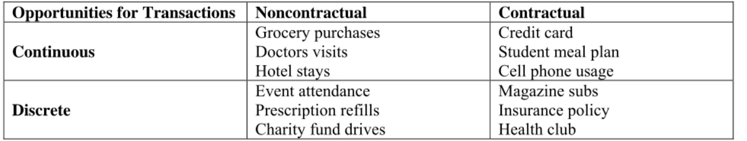
Fader Hardie, and Lee (2006 a) attempts to refine this categorization by considering contexts along two dimensions, i.e., “continuous-time and discrete-time” and “contractual and noncontractual”. It defines the notion of “continuous-time” where the customer-firm transaction can occur at any time, and “discrete-time” where transactions can occur only at discrete points in time. Also, it defines contractual case as one
14
where the time when a customer becomes inactive is observed and a noncontractual case as one where the time when a customer becomes inactive is not observed by the firm.4Based on these two dimensions (i.e., types of relationship with customers) it classifies customer base as shown in Table 1.
Table 1: Context Categorization proposed by Fader, Hardie, and Lee (2006 a)
Opportunities for Transactions Noncontractual Contractual Continuous
Grocery purchases Doctors visits Hotel stays
Credit card Student meal plan Cell phone usage
Discrete
Event attendance Prescription refills Charity fund drives
Magazine subs Insurance policy Health club
Although this categorization takes a significant step forward by using two dimensions, it can be refined further. It considers opportunities of transactions and customer defections because variations in customer behavior and the data available with the firm along these dimensions have significant implications for measuring CLV and the issues that become important for managers. However, spending by customers during a purchase occasion that is equally important has not been considered.
Let us focus on the discrete-noncontractual cell in Table 1. Prescription refills and Charity fund drives are both in this cell. However, for a relevant firm, the issues that are meaningful are not the same. In a charity fund drive, an organization soliciting funds has to make attempt to get funds, and get more of them. The amount donated can vary significantly from one occasion to another and across donors. In the prescription refill case, generally the amount remains the same or more predictable for any customer and similar to other customers with same illness. From a modeling point of view as well, a model of CLV in the case of charity fund drive is likely to include more complexity to deal with the uncertainty in the amount raised
4 Note that in Fader, Hardie, and Lee (2005 b), the definition of a noncontractual context would be the same as a
from a donor. The prescription refill case can do with a much simpler approach for modeling the spending component of the CLV model.
We believe that an adequate context categorization can result from a “bottom-up” approach that considers all the main drivers of CLV, namely, customer lifetime, interpurchase time, and spending. While the classification in Table 1 considers lifetime via the contractual-noncontractual dimension, and
interpurchase time via the continuous-discrete dimensions, it ignores the third critical dimension which is customer spending. Let us consider the money spent by a customer during each purchase occasion as falling into one of the following two categories: Fixed and Variable. In the Fixed category, the amount spent on each occasion is predictable easily, i.e., it is either the same or attains one of few possible discrete values and thus can be predicted relatively easily. For example, a magazine subscriber pays the same amount per time period for the magazine. In the Variable spending category, a customer can spend any amount.
For the firm in a context with Fixed spending, the issue of focus is the timing of purchase (i.e., interpurchase time) and/or customer defection (i.e., customer lifetime) whereas a firm in the Variable
spending category needs to focus on customer spending as well. From the point of view of estimating CLV, the latter (i.e., Variable spending) category poses more challenges. Examples of studies where spending falls in the Variable category are Borle, Singh, and Jain (2008) (where spending per transaction for each customer is modeled as Lognormal) and Fader, Hardie, and Lee (2005 a) (where spending per transaction is modeled as Gamma-Gamma).
Table 2 represents our refinement of the categorization in Table 1. Our aim is to propose a customer-firm relationship framework that adds to the existing framework in a meaningful manner and is reasonably comprehensive. It is noteworthy that a customer-firm transaction might not be monetary. For example, a
16
cell phone is used all the time which is a non-monetary transaction however payments for the phone services happen at fixed intervals. In developing the framework, we have focused on the monetary transactions as the key transactions of interest. This is reasonable because the timings of customer spending have a bearing on CLV and not the timing of product usage.5
Table 2: Proposed Context Categorization
Interpurchase Time Dimension
Customer Lifetime Dimension
Noncontractual Contractual Customer Spending Dimension
Fixed Variable Fixed Variable
Continuous (A) Offline movie rental (B) Grocery purchases Hotel stays Air travels (C) Student meal plan (D) Credit card Purchase clubs Discrete (E) Event attendance Prescription refills (F) Charity fund drives (G) Magazine subs Insurance policy Health club (H) Cell phone/PDA payments
Note: The examples in each cell are for illustration only and represent only the cases that are appropriate for the cell. Within each example, such as student mean plan, there could be examples that fall in another cell.
The context categorization presented in Table 2 is useful in understanding and prescribing models for use in a specific situation. Generally, it is most challenging to develop an accurate CLV model for context (B) and (D) where both the spending and interpurchase times are variable. Between these two, (B) presents a higher degree of difficulty due to lack of information about customer defection.
5 This is not to suggest that the timings of product usage do not affect CLV. Cost of managing customer
relationships, returns, etc. might occur at times different from the spending by a customer. These costs, if significant and when considered, would lead to further refinement of the categorization. Our purpose is to propose a
It is noteworthy that the two broad categories of the customer lifetime dimension (i.e., contractual and noncontractual) are the most interesting for modeling CLV. The other two components of a CLV model (i.e., spending and interpurchase time) can be suitably modeled relatively easily given the significant work in the general marketing literature on revenues from a customer and interpurchase time. Therefore, in presenting the models for CLV we focus on this lifetime dimension only. Any model proposed for a contractual or a noncontractual context can be modified relatively easily for use in any subcategory within these respective categories.
3.
Models for Measuring Customer Lifetime Value
In the general marketing literature, significant work has been done to investigate/forecast drivers of CLV such as customer lifetime, customer spending, interpurchase time, promotions and so on (e.g., Bolton 1998; Chintagunta 1993; Allenby, Leone, and Jen 1999; Bhattacharya 1998; Jain and Vilcassim 1991). As a result, numerous possibilities exist for combining models for different drivers of CLV to get its
estimate. In this section, we do not consider the individual models for a specific driver of CLV. Our focus here is on the prominent models proposed for estimating CLV. The CLV models that we discuss contain component models (or submodels) for the drivers of CLV considered. These submodels in turn are based on the extant research in the general marketing literature as mentioned earlier. Therefore, the CLV models discussed here have already considered the numerous possibilities for the component submodels, which justify our focus on these models only while ignoring the numerous other ad hoc possibilities.
We use the framework in Table 2 as a guide. To facilitate the descriptions, we categorize the models into two broad categories based on the context discussed earlier, namely, models for contractual and
noncontractual contexts. The models for each context can be modified suitably for use in any subcategory within the context. Therefore, a broad enough focus is more useful to keep the discussion parsimonious.
18
Table 3 presents the models that we discuss in this section. We first discuss models for contractual contexts followed by models for noncontractual contexts.
Table 3: Models of CLV discussed
CONTRACTUAL CONTEXT
1 Basic Structural Model of CLV (Jain and Singh 2002; Berger and Nasr 1998)
2 Regression/Recency, Frequency, and Monetary (RFM) Models (e.g., Donkers, Verhoef, and de Jong 2007) 3 Hazard Rate Models (Borle, Singh, and Jain 2008)
NONCONTRACTUAL CONTEXT
1 Pareto/NBD (Schmittlein, Morrison, and Colombo 1987)
2 Beta-Geometric/NBD or BG/NBD (Fader, Hardie, and Lee 2005 b)
3 Markov Chain Models (Pfeifer and Carraway 2000; Rust, Lemon, and Zeithaml 2004) 4 Markov Chain Monte Carlo (MCMC) Data Augmentation Based Estimation Framework (Singh, Borle, and Jain 2008)
3.1 Models for Contractual Contexts
In this context, firms know the time of customer defections. While a customer is in business with the firm, firms also have information on the realized purchase behavior of the customer. Donkers, Verhoef, and de Jong (2007) provide an excellent comparison of CLV models in a contractual context. Our discussion adds to their work. For a comprehensive picture of the models that can be used in a contractual context, we recommend reading both this section and Donkers et al. (2007). We first discuss the basic structural model of CLV now.
3.1.1 Basic structural model of CLV:
(
)
∑
= + − − = ni i i i d C R CLV 1 0.5 ) 1 (where i =the period of cash flow from customer transaction, Ri= revenue from the customer in period i,
Ci = total cost of generating the revenue Ri in period i, n = total number of periods of projected life of the
customer. Several variations of this basic model and their details can be found in Berger and Nasr (1998).
Using the basic structural model, one simple way to estimate CLV is to take the expected customer lifetime, the average inter-purchase time and dollar purchase amounts observed in the past and use them to predict the present value of future customer revenues assuming these average values for the inputs in the CLV model. Such a heuristic model would be a useful method to calculate customer lifetime value (CLV) in the absence of any better model (Borle, Singh, and Jain 2008).
Although the basic model (and its variations) is good to understand the essence of CLV, there are several issues with this formulation that relate to the assumptions it makes about customer purchase behavior. For example, it assumes fixed and known customer lifetime duration, revenues (both times and amounts), and costs of generating revenues. These restrictive assumptions make the model unattractive in most cases. Examples of cases where this model can be useful are newspaper or magazine subscriptions where the revenues from a customer are known and occur at fixed known times. The length of the subscription, i.e., customer lifetime, is the only unknown variable. The firm could use some rule of thumb for this length such as a fixed time period of say 3 years, or take the average subscription period for its past customers to get this time. Such simplistic measures will be biased but the low cost of applying this model might justify its use in the right situation.
In order to develop more accurate models one has to consider modeling customer lifetime better to reflect the variation in lifetime across customers. A good method would be to use hazard rate models for
20
modeling lifetime (Helsen and Schmittlein 1993). These models can provide more accurate information about the expected lifetime of each existing customer. This lifetime in turn can be used in the CLV models along with the revenues and cost information to get an estimate of the lifetime value of each customer. The models discussed in this section so far are most suitable for the cases that fall in cell (G) in
Table 2. In other situations within the contractual context, the assumptions of fixed revenues and costs cannot be justified. Therefore, researchers have developed ways to make the basic model more flexible or find alternatives to it.
3.1.2 Regression/RFM Models:
The regression/RFM methods are commonly used techniques to score customers for a variety of purposes (e.g. targeting customers for a direct mail campaign). An RFM framework uses information on a
customer’s past purchase behavior along three dimensions (recency of past purchase, frequency of past purchases, and the monetary value of past purchase) to “score” customers. Regression methods can use these and other variables as well to score customers as well as estimate CLV of each customer. The scores are related to the expected potential customer purchase behavior and hence can be considered as another measure of customer value to the firm. Scores generally serve a similar purpose as the CLV measure. Although we have discussed these methods in this section, they have been used in noncontractual contexts as well. Examples of application of such methods can be found in (Borle, Singh, and Jain 2008; Donkers, Verhoef, and de Jong 2007; Malthouse and Blattberg 2005; Reinartz and Kumar 2003; Colombo and Jiang 1999).
3.1.3 Hazard Rate Models:
Jain and Vilcassim (1991) and Helsen and Schmittlein (1993) provide a good introduction of hazard rate models in marketing. Hazard of an event means the risk of an event. Here, the event is customer defection or purchase. These models are well suited to model the risk of customer defection and the risk of purchase
happening when data about these events is available. The estimates from these models in turn provide the expected duration of customer lifetime and interpurchase time. Depending upon the characteristics of customer spending, a suitable model can be used for its estimation. The estimates from these three submodels (i.e., lifetime, interpurchase time, and spending) can provide estimates of CLV. A prominent example of this approach in a contractual context is provided in Borle, Singh, and Jain (2008) that we refer to as the BSJ 2008 model henceforth.
The BSJ 2008 Model:
This hierarchical Bayesian model proposed in Borle, Singh, and Jain (2008) jointly predicts a customer’s risk of defection, risk or purchase, and spending, at each purchase occasion. This information is then used to estimate the lifetime value of each customer of the firm at every purchase occasion. The firm can use this customer lifetime value information to segment customers and target them. Borle, Singh, and Jain (2008) develops and applies the model to data from a direct marketing company. It tests the model and shows that it performs significantly better in both predicting CLV and targeting valuable customers than a simple heuristic model, an advanced RFM model proposed by Reinartz and Kumar (2003), and two other models nested within the proposed BSJ 2008 model.
The BSJ 2008 model is a joint model of the three dependent drivers of CLV, namely the inter-purchase time, the purchase amount and the probability of leaving given that a customer has survived a particular purchase occasion (i.e., the hazard rate or the risk of defection). The model for each of these three quantities is specified along with a correlation structure across these three submodels leading to a joint model of these three quantities. In the model, the interpurchase time is assumed to follow a NBD process, the amount expended by a customer on a purchase occasion follows a lognormal process, and the hazard of lifetime i.e., the risk of customer defection in a particular interpurchase time spell is modeled using a discrete hazard model. The model also incorporates time-varying effects to improve the predictive
22
performance. Please see Borle, Singh, and Jain (2008) for more information. We now discuss models for noncontractual contexts.
3.2 CLV Models for Noncontractual Contexts
In this context, firms do not know whether a customer has defected or intends to remain in business with the firm. Since knowledge of customer lifetime is essential to estimate CLV, this becomes a challenging context for CLV measurement. Some users deal with this challenge by considering a future time period of a fixed duration, say 3 years and estimating the net present value of the profits from a customer during this period. The user can use regression models to estimate future timing and amount of spending by the customer during this period. Past purchase behavior and customer characteristics are some of the variables that can be included as explanatory variables in the regression model. Such methods can be applied in many ways (e.g., Malthouse and Blattberg 2005). It is noteworthy that such ad hoc approaches are best suited for forecasting an outcome during the next time period. As the forecasting horizon
increases, these methods produce more error.
The following discussion focuses primarily on stochastic models of CLV that assume some underlying customer purchase behavior characteristics. These models assume that the observed customer purchase behavior is generated due to these latent customer characteristics. Such models have advantages over other approaches as discussed in detail in Fader, Hardie, and Lee (2006 a).
3.2.1 The Pareto/NBD Model:
The Pareto/NBD model was developed by Schmittlein, Morrison, and Colombo (1987). The model uses observed past purchase behavior of customers to forecast their likely future purchase behavior. This
outcome is then used as input to estimate CLV (e.g., Reinartz and Kumar 2000 and 2003; Fader, Hardie, and Lee 2005 a; Singh, Borle, and Jain 2008).
When customer defections are not observed, the Pareto/NBD model is a very elegant way of getting the probability of a customer being alive in a relationship with a firm. This model can be used to estimate (a) the number of customers currently active; (b) how this number changes over time; (c) the likelihood of a specific customer being active; (e) how long is a customer likely to remain an active customer; and (f) the expected number of purchases from a customer during a future time interval. The model assumptions are as follows.
Model Assumptions:
a. While the customer is active in business relationship with the firm, he/she makes transactions with the firm that are randomly distributed in time with customer –specific rate λ. Therefore, the number of transactions X made by a customer in time period of length t is a Poisson random variable.
b. A customer has unobserved lifetime duration represented by τ which is an exponential random variable. Customer’s dropout or defect from the firm randomly according to a rate µ. c. The transaction rate λ follows a Gamma distribution across customers with parameters r, α>0.
The mean purchase rate across customers is E[λ]=r/α and the variance is r/α2.
d. The dropout rate µ follows a Gamma distribution across customers with parameters s, β>0. The mean dropout rate is E[µ] = s/β and the variance is s/β2.
e. The purchase rates λ and dropout rate µ vary independently across customers.
For a customer, the expected number of transactions made in T units of time following an initial purchase is
24
(
)
⎥
⎥
⎦
⎤
⎢
⎢
⎣
⎡
⎟⎟
⎠
⎞
⎜⎜
⎝
⎛
+
−
−
=
−11
1
]
,
,
,
,
/
[
sT
s
r
T
s
r
X
E
β
β
α
β
β
α
For α>β, the probability that a customer is still active, given an observed purchase history of X purchases in time (0,T) since the initial purchase with the latest purchase happening at time t is
(
)
(
( )
)
( )
(
)
1 1 1 1 1 1 1 1 1 ; ; , ; ; , 1 , , , , , , / − + ⎪ ⎪ ⎭ ⎪ ⎪ ⎬ ⎫ ⎪ ⎪ ⎩ ⎪ ⎪ ⎨ ⎧ ⎥ ⎥ ⎥ ⎥ ⎥ ⎦ ⎤ ⎢ ⎢ ⎢ ⎢ ⎢ ⎣ ⎡ ⎟ ⎠ ⎞ ⎜ ⎝ ⎛ + + − ⎟ ⎠ ⎞ ⎜ ⎝ ⎛ + + ⎟ ⎠ ⎞ ⎜ ⎝ ⎛ + + + + + = = T z c b a F T T t z c b a F t T t T s x r s T t x X s r Alive P s s x rα
β
α
β
α
α
β
α
where a1 = r + x + s; b1 = s + 1; c1 = r + x + s + 1; z1(y) = (α-β)/(α+y). For cases when α = β and α < β,
please see Schmittlein, Morrison, and Colombo (1987).
Extended Pareto/NBD Model: Schmittlein and Peterson (1994) empirically validate the Pareto/NBD
model and propose an extension to it by incorporating dollar volume of purchase. The key assumption here is that the distribution of average amount spent across customers is independent of the distribution of the transaction rate λ and the dropout rate µ. The expected future dollar volume per reorder is provided in Schmittlein and Peterson (1994). Note that for the estimation of CLV, the output of the Pareto/NBD model is used along with the output from a suitable model for customer spending.
Despite the significant merits of the Pareto/NBD model, it imposes strong assumptions on the underlying customer purchase behavior that might not be suitable for many situations (Borle, Singh, and Jain 2008). In addition, it is somewhat difficult to estimate as recommended thus restricting its usage in practice. Several researchers have attempted to generalize the Pareto/NBD model and/or suggest alternatives that are easier to estimate. For example, Abe (2008) extends the Pareto/NBD model using a hierarchical Bayesian (HB) framework. The extension maintains the three key assumptions of the Pareto/NBD model,
i.e., a Poisson purchase process, a memoryless dropout process, and heterogeneity across customers, and relaxes the independence assumption of the purchase and dropout rates.
3.2.2 The BG/NBD Model:
Proposed by Fader, Hardie, and Lee (2005 b) as an “easy to estimate” alternative to the Pareto/NBD model, the Beta-Geometric-NBD (BG/NBD) model makes slightly different assumptions about the underlying customer purchase behavior that make it significantly easier to implement and yet allow the user to obtain similar benefits. If ease of estimation is desired, the BG/NBD model is an excellent alternative to the well known Pareto/NBD model.
The assumptions underlying the BG/NBD model are as follows:
a. While active, the number of transactions made by a customer follows a Poisson process with transaction rate λ. Therefore, the time between transactions follows exponential distribution. b. λ follows Gamma distribution across customers with parameters r and α.
c. After any transaction a customer defects (becomes inactive) with probability p. Therefore the customer dropout is distributed across transactions as a (shifted) geometric distribution. d. p follows a beta distribution with parameters a and b.
e. λ and p vary independently across customers.
Note that assumptions (a) and (b) are identical to the Pareto/NBD model. While the Pareto/NBD model assumes that customers can defect at any time, the BG/NBD model assumes that defections occur immediately after a purchase. Using these assumptions, the expression for the expected number of transactions in a future time period of length t for an individual with observed past purchase behavior is obtained as
26
( )
(
)
r x x x x r x t T x b a t T t x b a x b x r F t T T a x b a b a r T t x X t Y E + > + ⎟⎟ ⎠ ⎞ ⎜⎜ ⎝ ⎛ + + − + + ⎥ ⎥ ⎦ ⎤ ⎢ ⎢ ⎣ ⎡ ⎟ ⎠ ⎞ ⎜ ⎝ ⎛ + + − + + + + ⎟ ⎠ ⎞ ⎜ ⎝ ⎛ + + + − − − + + = = α α δ α α α α 1 1 ; 1 ; , 1 1 1 , , , , , , / 0 1 2 where(
)
(
−)
∫
( ) (
− −)
> = 1 − −− − 0 1 1 1 2 1 1 , c b , 1 ; ; , t t zt dt b c b B z c b aF b c b a , is the Euler’s integral for the
Gaussian hypergeometric function, x is the number of transactions observed in time period (0,T] and tx (0
< tx≤ T) is the time of the last transaction.
Please see Fader, Hardie, and Lee (2005 b) for more details of the BG/NBD model. The article also compares the forecast of future purchasing using the BG/NBD model with that from the Pareto/NBD model and finds that both the models are accurate (both at the individual customer level and the aggregate level). Just as in the case of Pareto/NBD model, the outcome from the BG/NBD model in combination with the outcome from a suitable customer spending model can be used to estimate CLV of each customer.
3.2.3 MCMC Based Data Augmentation Algorithm by Singh, Borle, and Jain (2008):
The Pareto/NBD, the BG/NBD, and the Abe (2008) models discussed so far in this section have several advantages over the earlier used RFM scoring methods. The key advantages accrue as a result of the behavioral story underlying these models where the observed transactions are considered a manifestation of underlying latent customer characteristics (see Fader, Hardie, and Lee 2006 a). The problem is that the “story” underlying the modeling approach so far has been limited to strict assumptions imposed on customer characteristics such as the purchase behavior. For example, the Pareto/NBD model assumes that individual customer lifetimes and interpurchase times follow different exponential distributions. This is a restrictive assumption that might not be supported in many situations. In addition, the model assumes that
the outcomes of lifetime, interpurchase time, and spending are independent of each other. Since these outcomes belong to each customer, the assumption of independence between these outcomes is also restrictive. Finally, the estimation of these models (except the BG/NBD model) is challenging. The Markov Chain Monte Carlo (MCMC) based data augmentation framework proposed by Singh, Borle, and Jain (2008) (henceforth referred to as the SBJ framework for simplicity) addresses these issues
successfully.
The SBJ framework at its core has an algorithm for estimating CLV models in noncontractual contexts, and is not a specific model. Therefore it is fundamentally different from the models proposed so far in the literature. The SBJ framework can be used to estimate all the models discussed so far in addition to many different models with varying distributional assumptions for the underlying customer behavior. In fact any standard statistical distribution can be used for the underlying customer characteristics generating the data. Therefore the user is not restricted to assuming that the interpurchase times and lifetimes follow exponential distributions. The algorithm then allows forecast of future purchase transactions and the CLV using these.
Both the Pareto/NBD and the BG/NBD models assume that the underlying drivers of CLV (i.e., customer lifetime and interpurchase time) are independent. Also, when these models are used for estimating CLV by adding a model for customer spending, spending too is assumed to be independent of these other behaviors. In reality, this independence is very hard to justify as these outcomes are for the same customer. The SBJ framework allows for the estimation of correlation between the defection, purchase, and spending outcomes. Please see Singh, Borle, and Jain (2008) for applications of the framework including the estimation of the extended Pareto/NBD model, the BG/NBD model, and a number of other models that use different underlying distributions for customer lifetime and purchase behavior. The article finds that the assumptions of more flexible distributions for the underlying customer behavior yield more
28
accurate forecast. Some models compared yield significantly better performance that the Pareto/NBD and the BG/NBD underscoring the value of the framework. It is noteworthy that such flexibility in modeling of CLV in noncontractual contexts was not available to the users earlier. The advantages of the SBJ framework over existing alternatives are very significant and we recommend its usage for forecasting customer purchase behavior in this context.
We now describe the key algorithm in the SBJ framework using the example of the Pareto/NBD model. If we assume that customer purchase behavior follows the assumptions underlying the Pareto/NBD model and use the SBJ framework to estimate the Pareto/NBD model, the assumptions and the simulation/data augmentation steps involved are as shown in Tables 4 and 5:
Table 4: Notation used in the framework (using Pareto/NBD assumptions)
Notation Explanation
h A particular customer.
Th The total time for a customer h from the initial purchase occasion until the current time.
th The time from the initial purchase occasion until the last observed purchase occasion for customer h (Therefore th ≤ Th).
Xh The total number of purchases made by customer h since the initial purchase in time period Th, with the latest purchase being at time th.
IPThi The interpurchase time between the ith and the (i-1)th purchase for customer h.
totLIFEh Total lifetime of customer h from the initial purchase occasion until the customer defects. This is a latent variable, i.e. unobserved by the firm.
totLIFEh(old) and
totLIFEh(new)
Intermediate variables used in the simulation of the latent variable totLIFEh
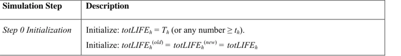
Table 5: Simulation/data augmentation steps involved in estimating the Pareto/NBD model using the SBJ algorithm
Simulation Step Description
Step 0Initialization Initialize: totLIFEh = Th (or any number ≥th). Initialize: totLIFEh(old) = totLIFEh(new) = totLIFEh
Initialize: The parameters(r,α)and(s,β)
Step 1 Draw totLIFEh(new) (such that totLIFEh(new)≥ th) from the Pareto distribution with the current parameters (s,β)
Step 2 Calculate two likelihoods for each customer—likeh(old) is the likelihood of the interpurchase time data for customer h conditional on the lifetime of h being
totLIFEh(old), and likeh(new) is the likelihood of the interpurchase time data for customer h conditional on the lifetime of h being totLIFEh(new) drawn in the previous step.
Step 3
Assign totLIFEh = totLIFEh(new) with probability ( ) ( ) ) ( old h new h new h h
like
like
like
prob
+
=
,else assign totLIFEh = totLIFEh(old)
Step 4 Estimate the Pareto distribution parameters (s,β) and the NBD distribution
parameters (r,α)conditioning on the total lifetime of the customer h being totLIFEh. That is, update NBD parameters (r,α)and Pareto parameters (s,β)
Step 5 Set totLIFEh(old) = totLIFEh Step 6 Go to Step 1
Source: Singh, Borle, and Jain (2008).
To estimate CLV, a model for customer spending is required as well. Please see Singh, Borle, and Jain (2008) for more details regarding estimating CLV using the framework, and modeling of covariates and correlations between the outcomes. The paper also shows many other application of the framework using different distributional assumptions for the drivers of CLV.
3.2.4 Markov Chain Models:
Markov chain models have been used in marketing for years to model brand switching (e.g., Kalwani and Morrison 1977). Their flexibility and ability to model competition allows their use in modeling CLV as well. Suitable modifications of these models can be used both in a contractual and noncontractual context. An early use of this class of models for modeling CLV can be found in Pfeifer and Carraway (2000) who illustrate the relationship between markov chain models and the commonly used recency, frequency, and
30
monetary (RFM) framework. Rust, Lemon, and Zeithaml (2004) presents a relatively sophisticated version of a markov chain model to model CLV that we discuss now.
Customer Equity Model of Rust, Lemon, and Zeithaml (2004):
When data is available from multiple vendors that compete for the same set of customers, this model is a very nice option for modeling the lifetime value of customers for specific brand/vendor. The flexibility of the model allows estimation of the impact of several drivers of customer lifetime value on the total lifetime value of a firm’s customers as well as that of its competitors. Another advantage of the model is that it can be estimated using cross sectional survey data as well as longitudinal panel data.
Using individual-level data from a cross-sectional sample of customers, combining it with purchase or purchase intentions data, each customer’s switching matrix is modeled. The individual choice
probabilities in the switching matrix, i.e. the probability that individual i chooses brand k given that brand
j was most recently chosen, is modeled using multinomial logit model. Therefore, each customer i has a
JXJ switching matrix where J is the number of brands.
The lifetime value of customer i to brand j is then calculated using these probabilities, the average purchase rate per unit time, the average purchase volume for brand j, and the per unit contribution margin for brand j. The other details can be found in Rust, Lemon, and Zeithaml (2004).
4.
Key Issues in Modeling CLV
The literature on CLV models has exploded in the past few years. So far, the models proposed to estimate CLV have generally considered the revenue stream from customers and some obvious costs involved. Underlying this revenue stream there are many complex and important factors that have generally not
been considered in depth while modeling CLV. In addition, there are other factors related to the customer that are still not well understood, and that can benefit the firm (e.g., network effects).
Consider revenues from a customer. These revenues might come from purchases in multiple categories and customer purchase behavior with respect to each category might vary. They might come in response to promotions with varying costs and effectiveness. Examples of such factors that can impact CLV are cross-selling, word-of-mouth effect, returns, and marketing actions and their impact on the revenues from different sources. To estimate CLV, one could potentially forecast the revenues directly using some sort of model for total revenues or one could model the revenues due to each underlying factor, such as purchases in each category, and build up the forecast for the total revenues.
Some other areas in marketing have focused on many of these underlying customer-level factors to understand and forecast them better (e.g., Hess and Mayhew 1997). However, within the CLV
measurement literature, models proposed so far have generally explicitly or implicitly made assumptions about many of these factors to deal with them. These assumptions take various forms such as a factor having no impact (i.e., when it is ignored) or a factor having the average value for all customers (e.g., Kumer, Ramani, and Bohling 2004). To take the CLV literature forward, bridges have to be built between the research on the drivers of CLV (and the factors that impact these drivers) and the literature on CLV measurement models such that the CLV measurement models can be refined further to provide better understanding of the effect of various factors on CLV and to forecast CLV more accurately. In this section we now discuss some of the key issues that need to be considered in models of CLV to advance the CLV measurement literature.
32
In analyzing the return on investment in customer relationships, how much a firm spends on acquiring a new customer is an important consideration. Acquiring customers at a price more than their lifetime value (i.e., acquiring customers with negative PLV) would obviously result in a loss. It is common to see the popular press talk about the average cost of acquiring a customer is a specific industry (e.g., Schmid 2001), however such average figures could be misleading. Experience of many direct marketing companies suggests that while some customers are quick to start business with the firm, others are reluctant and need many solicitations before starting business with the firm. Clearly then the cost of acquiring different customers can be different. Once acquired, how does the purchase behavior (and subsequently the lifetime value) of these different customers differ?
Research suggests that the value of customers acquired though different channels can be different
(Villanueva, Yoo, and Hanssens 2008; Lewis 2006). For example, Villanueva, Yoo, and Hanssens (2008) using a Web hosting company data finds that customers acquired through costly but fast-acting
marketing investments add more short-term value and customers acquired via word-of-mouth add nearly twice as much long-term value to the firm. Some other studies have linked acquisition and retention (e.g., Blattberg and Deighton 1996; Thomas 2001; Reinartz, Thomas, and Kumar 2005), however, to our knowledge no one has considered the total cost of individual customer acquisition (e.g., cost attributable to the channel of acquisition and promotions for acquisition) with the subsequent customer purchase behavior and CLV. The heterogeneity in the cost of acquiring different customers needs more research and should be accounted for in evaluating prospects.
2. Cost of Customer Relationship Management:
Once a prospect has been acquired as a customer, firms spend resources for managing relationship with the customer and selling to him/her. These resources involve costs that can be complex and hard to pin point. For example, while the cost of manufacturing a product or those associated with promotions are
relatively easier to obtain, the cost of employee time on an activity or the cost of managing returns are difficult to estimate. Since information about costs is generally not available to a researcher easily, most models of CLV make assumptions about these costs.
For example, Venkatesan and Kumar (2004) while discussing cost say that “The discounting of cost allocations is straightforward if we assume that there is a yearly allocation of resources (as is the case in most organizations) and that the cost allocation occurs at the beginning of the year (the present period).” The issue is that many organizations have aggregate cost figures and allocating them in any model for individual customers without considering the variation in costs across them is likely to provide biased CLV estimates. Research suggests that such average cost allocation might not be appropriate as cost of serving a customer might be different for different customer (see Reichheld and Teal 1996).
Some studies focus on net revenues from customers and ignore the cost part altogether due to lack of availability of cost data. For example, Borle, Singh, and Jain (2008) propose a sophisticated model for measuring CLV in a contractual context. Due to unavailability of cost data they use net spending by customers to apply their model. Although their approach can be modified easily to include cost data as well, application of their model without such cost data can reduce the accuracy of the model forecasts.
The cost of managing customer relationships and selling to them has several different sources. Following are some of the key sources that need consideration:
Cost of Customer Retention: Firms take various initiatives such as loyalty programs to retain customers.
The cost of such loyalty programs has yet to be adequately considered in models for CLV. This cost includes the cost of designing the program, launching it, and managing it in an ongoing fashion. While the first two components are part of the fixed cost of such programs and can be ignored, the cost of
34
managing the program is variable and should be considered if possible in evaluating customers. Within these cost components there is the cost of physical and employee resources expended. Given that CLV is a customer level measure, how does one allocate these costs to an individual customer? Should it be allocated equally or should some other factor such as the frequency of product usage, the time spent with a customer service representative, or a combination of these form the basis of cost allocation? To our knowledge, these questions have not been considered in this literature.
Cost of Marketing Activities: It is common to see models consider marketing activities as explanatory
variables in models for measuring CLV. The cost of such activities however is generally ignored. This cost might vary across customers and a model has to account for this variation to accurately forecast CLV (Kumar, Shah, and Venkatesan 2006). For example, while some customers would be sent many
promotions before they make a purchase, others might require just one.
Cost of Returns: Returns by customers has generally been ignored in developing CLV models. Given its
importance, we discuss it in greater detail here.
Return of purchased product by a customer is an undesirable activity for both the customer and the firm. Customers return an estimated $100 billion worth of products each year. The reasons for this trend include the rise of electronic retailing, the increase in catalogue purchases, and a lower tolerance among buyers for imperfection (Stock, Speh, and Shear, 2002). Hess and Mayhew, (1997) suggest that in direct marketing, the fact that customers do not physically evaluate a product before purchasing increases the risk of returns. Further, direct marketers should expect 4-25% of their sales returned. It is clear that returns are important but this importance is not reflected in the research output related to product returns.
In the CLV literature, some researchers have used returns as explanatory variables in a model for a specific driver of CLV (e.g., Venkatesan and Kumar 2004; Reinartz and Kumar 2003), however, returns have not been incorporated in CLV measurement models directly despite being one of its key drivers. Demonstrating the value of returns for measuring CLV, Singh and Jain (2008) uses data from a direct marketing company to segment customers on the basis of purchases and returns. It then estimates segment level CLV first while ignoring returns and then while accounting for returns by individual customers. It finds that consideration of returns significantly alters CLV. One segment of customers that is very attractive when returns are ignored becomes highly unattractive when returns are accounted for. The impact of returns on CLV varies significantly across segments underscoring the need for considering returns at the individual customer level in modeling CLV.
3. Cross-selling:
Many businesses such as retailers (e.g., Amazon.com), consumer products companies (e.g., Johnson & Johnson), banks (e.g., Citibank), and insurance companies (e.g., Allstate) attempt to sell different types of products and services to their existing customers. For example, consider a customer who purchases a digital camera from Amazon.com. As soon as she purchases the digital camera, she gets personalized promotions of camera accessories such as a camera bag from Amazon.com. These cross-selling opportunities to a customer are an important reason for firms investing in customer retention. If a firm acquires a customer who buys from one division, the firm has information about the customer and her purchase behavior that can be used to its advantage by more effectively selling other products/services to the customer. Further, cross-selling enhances customer retention due to higher switching costs for customers who purchase multiple products and services from a firm (Kumar, George, and Pancras 2008). This implies that cross-selling to customers is likely to increase revenues and reduce the cost of customer retention. Therefore, for the firm, part of the customer value lies in the potential for cross-selling.
36
The importance of cross-selling to customer value is well recognized by researchers (Kumar, George, and Pancras 2008; Verhoef and Donkers 2005; Ngobo 2004; Venkatesan and Kumar 2004; Reinartz and Kumar 2003; Blattberg, Getz, and Thomas 2001; Verhoef, Philip, and Hoekstra 2001; Kamakura, Ramaswami, and Srivastava 1991). However, how to measure and incorporate the cross-selling potential of a customer (that is likely to vary across customers) into CLV models remains a research question.
4. Word of Mouth Effect:
Word-of-mouth represents informal communication between customers/consumers about a firm and/or its product and services (Tax, Chandrashekaran, and Christiansen 1993). Such communication can be both positive and negative. The value of customer word-of-mouth for a firm is well recognized (Zeithaml 2000; Harrison-Walker 2001; Helm 2003; Rogers 1995; Danaher and Rust 1996; Herr, Kardes, and Kim 1991; Walker 1995; Murray 1991; Buttle 1998). The importance of customer referrals for new customer acquisition is also recognized by researchers (Mangold, Miller, Brockway 1999; Rogers 1995). The popularity of referral reward programs and viral marketing programs in practice reflects the value firms place on word-of-mouth effects. While some researchers have attempted to estimate word-of-mouth effects, the research is still in its early stages due to the complexity involved (e. g. Helm, 2003; Hogan, Lemon, and Libai 2004 ). Kumar, Petersen, and Leone (2007) use data from a telecommunications company and financial services firm to estimate the value of customer referrals and conclude that a firm’s best marketers may be worth far more to the firm than the most enthusiastic customers thus highlighting the importance of word-of-mouth in evaluating customers.
Despite the importance of word-of-mouth effects, it is only recently that these and other network effects (e.g., participation in customer communities) have started getting the attention of researchers in CLV (e.g. Lee, Lee, and Feick 2006; Kumar, Peterson, and Leone 2007; Hogan, lemon, and Libai 2004). It is obvious that these factors have an impact on customer value. What is not obvious is how to incorporate