A Simple Repeat Sales House Price Index: Comparative Properties Under Alternative Data Generation Processes.

A Simple Repeat Sales House Price

Index: Comparative Properties Under

Alternative Data Generation Processes

Arthur Grimes and Chris Young

Motu Economic and Public Policy Research September 2010

Author contact details

Motu Economic and Public Policy Research; and University of Waikato [email protected]

Chris Young

Motu Economic and Public Policy Research [email protected]

Acknowledgements

We thank the Foundation for Research, Science and Technology for funding assistance (FRST grant MOTU-0601 Infrastructure) and Steve Stillman, Dave Maré and Andrew Coleman for suggestions. We also thank Wei Zhang for assistance. The authors, however, are solely responsible for the views expressed.

Motu Economic and Public Policy Research

© 2010 Motu Economic and Public Policy Research Trust and the authors. Short extracts, not exceeding two paragraphs, may be quoted provided clear attribution is given. Motu Working Papers are research materials circulated by their authors for purposes of information and discussion. They have not necessarily undergone formal peer review or editorial treatment. ISSN 1176-2667 (Print), ISSN 1177-9047 (Online).

Abstract

We propose a new method to estimate a repeat-sales house price index. Our unbalanced panel method employs an OLS panel regression to estimate the (log) house price as a function of time fixed effects and house-specific fixed effects. Comparisons are made across three repeat-sales methods using actual data, and using simulated data with both stationary and non-stationary relative price innovations. The unbalanced panel method comprehensively utilises all sale information on a house rather than splitting sales into distinct pairs. It is the simplest of the methods to implement, and possesses superior properties to the other two methods under a wide range of data generation processes.

JEL codes

Keywords

Contents

1. Introduction ... 1

2. Prior Methods ... 1

3. Unbalanced Panel Method ... 4

4. Repeat-Sales House Price Index Comparison ... 5

4.1. Actual data ... 5

4.2. Simulated data ... 6

5. Conclusions ... 13

References ... 15

Appendix 1: House Price Index Results ... 16

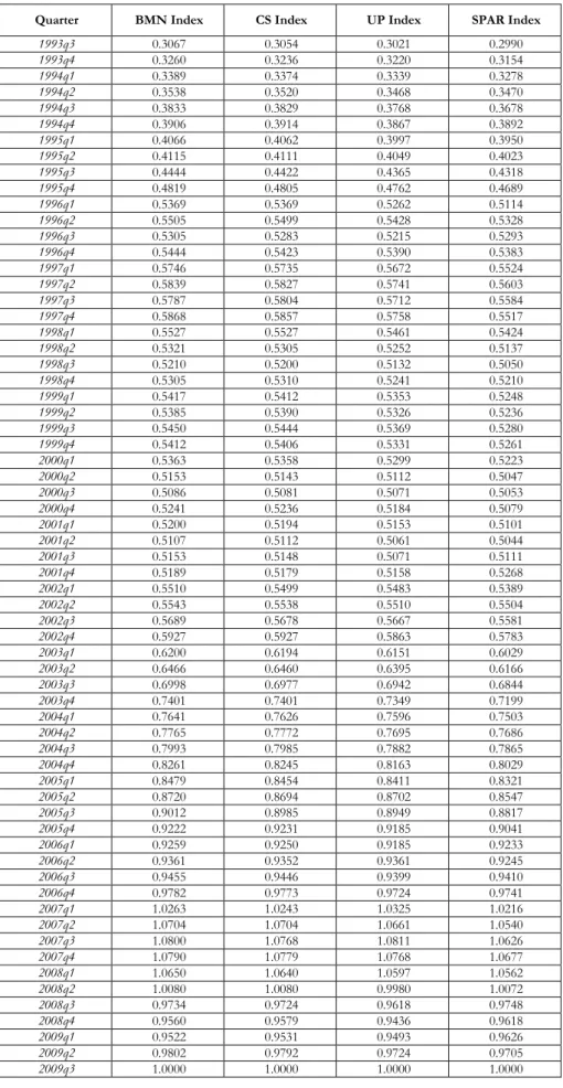
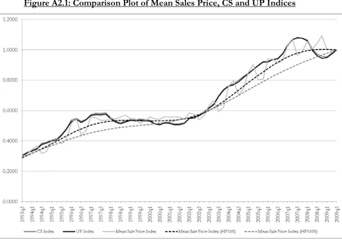
Appendix 2: Mean and Median Sales Price Comparison ... 19

1.

Introduction

Availability of a reliable house price index is vital for policy-makers, real estate and financial markets participants, and researchers into housing, macroeconomic and regional issues. House prices are volatile at both the micro and macro levels, and estimation of an index is complicated by the fact that individual houses are sold infrequently and that the composition of houses sold varies across time. These factors complicate the process of estimating a house price index that represents the “true” path of house prices in a given area over time.

Several methods have been proposed for producing a house price index. These include simple (mean and median) measures, hedonic pricing models, and repeat-sales methods. We focus on repeat-sales methods and propose a new method to estimate a repeat-sales index: the unbalanced panel method. This method utilises an OLS panel regression of log house price on a set of time fixed effects and house-specific fixed effects. It has the advantage over prior methods that it utilises all sale information on a house in a comprehensive manner rather than separating out distinct pairs of sales as in prior methods.

We compare the unbalanced panel method with methods proposed by Bailey et al (1963) and Case and Shiller (1987). We initially estimate house price indices using all three methods using actual repeat-sales data, observing that the estimated indices are very similar to each other; they are also similar to the related SPAR index proposed by Bourassa et al (2006). In order to rank the alternative repeat-sales methods, we estimate indices using each method based on simulated data with three different data generation processes (DGPs): serially uncorrelated, mean-reverting and a random walk. The unbalanced panel method is generally superior (i.e. more accurate over the whole period and within each period) to the other methods across a range of simulated DGPs, except where relative house prices follow a (near) random walk; this result is robust to changes in sales numbers and sample length. Furthermore, the unbalanced panel method is by far the easiest of the three methods to implement.

Section 2 of the paper provides a brief survey of prior methods to estimating house price indices. Section 3 describes the unbalanced panel method, before we compare the various methods in Section 4. Conclusions follow in Section 5.

2.

Prior Methods

A reliable house price index is required to measure housing market trends. A number of methods have been employed to produce such an index. One set of methods uses simple summary measures, such as the mean or median house sales price, to formulate an index. The

flaw of this approach is that there is no adjustment made for quality of houses sold; thus the measure cannot distinguish whether there has been an actual change in house price level or whether the change in observed prices is due to a different mix (quality) of houses sold.

A second set of methods is based on an hedonic regression equation. The premise is that observed house characteristics can be accurately used to predict the house price. House sale prices are regressed on a set of variables describing the characteristics of each house, and on a set of time fixed effects. The time fixed effects are used to compile the house price index, while the coefficients on the characteristic variables act like shadow prices, indicating the change in house price for a marginal change in a characteristic. Major challenges in using the hedonic method include specifying the correct functional form for the model, determining the correct set of explanatory variables, and obtaining data to accurately represent all relevant characteristics.

A third approach is to use a repeat-sales method, first proposed by Bailey et al (1963). The repeat-sales method uses data on properties that have been sold at least twice. The benefits of using a repeat-sales method are that it uses repeat observations of single housing units; thus, it controls for house characteristics more accurately than does the hedonic method which relies on the quality of measurement of housing characteristics (McMillen and McDonald, 2004). The only assumption is that the quality of individual houses remains constant over time (Case and Shiller, 1987). Reduced sample sizes and selection bias are two potential flaws of this method; the repeat-sales method only uses observations of houses that have sold more than once, meaning only a proportion of house sales are kept in the sample.

Bailey et al implement their repeat-sales method by using pooled ordinary least squares (OLS) to regress the difference in log house price, between the second and first sale, on a set of dummy variables; one for each time period in the sample except the first (base) period. Each dummy variable takes the value zero, excluding the two dummies corresponding to a sale period; the second sale period dummy takes value +1, while the dummy corresponding to the first sale period takes value -1. If the first sale period coincides with the base period, then there is no dummy corresponding to the first sale. The estimated coefficients on the dummy variables can be interpreted as the log house price index. Bailey et al estimate the following equation:

∑

where HPit is the sale price of house i in period t ; k and j represent the periods in which

the second and first sale occurred, respectively; rt represents the rate of appreciation in the house

Bailey et al assume that the variance of the error term in their model is constant, i.e. independent of the time between adjacent sales. Case and Shiller (1987) argue that the variance is likely to be related to the length of time between two sales. They suppose that there exists a random drift through time of house prices, due to unexplainable differences in the levels of maintenance across houses, or random changes in neighbourhood quality. Hence, Case and Shiller construct a weighted repeat-sales (WRS) index that accords houses sold after longer periods of time less weight in index construction.1

lnHPit = Ct + Hit + Nit (2)

They assume the log price of house i at time t

is given by:

where Ctis the log of the city-wide level of house prices at time t; Hit is a random walk

term that represents the drift in house prices over time (ΔHit has zero mean and constant

variance σh2; Hitis uncorrelated with Ctand Nit); and Nit is a sale specific, serially uncorrelated

random error term, with zero mean and constant variance σN2 for all i.

The goal of Case and Shiller was to estimate the movement in C, the city-wide level of house prices. The WRS method comprises three stages. The first stage is to estimate the Bailey et al regression model of differenced log house prices on the set of time dummy variables. A vector of regression residuals is obtained and a regression of the square of these residuals is run on a constant and the time interval between sales as the second stage. The constant term of the second stage regression is an estimate of 2σN2, and the slope coefficient is an estimate of σh2. The

third stage is a weighted generalized least squares regression of the first stage equation after each observation has been divided through by the square root of the fitted values from the second stage regression.2

Jansen et al (2008) also implement a WRS model, constructed similarly to that of Case and Shiller. As suggested by Abraham and Schaumann (1991), they include a quadratic time term into their second stage regression to account for the possibility that the variance of the error term may not necessarily increase linearly, but instead decrease as the period between sales increases.

An alternative index to both the hedonic and repeat-sales indices, suggested by Bourassa et al (2006), is a sale price appraisal ratio (SPAR) index. Like the repeat-sales index, the SPAR index is based on matched pairs, but it is not restricted to properties that have sold at least twice.

1 _{The Case-Shiller method (that underlies the S&P/Case-Shiller Home Price Indexes) forms the basis for the}

housing futures and options contracts on the Chicago Mercantile Exchange.

2 _{Goetzmann (1992) proposed an ex-post correction to the Case and Shiller model (adding half the variance in the} house price growth rate associated with the diffusion of house prices over time) to take account of the log transformation downwardly biasing the arithmetic mean. Wang and Zorn (1997) discuss the importance of heteroskedasticity in relation to the purposes of index construction.

This reduces the sample selection bias and sample size issue from which a repeat-sales method may suffer. The SPAR method uses the appraisal values (for property tax purposes) of each property to estimate the base period sales prices. The use of an appraised value, rather than a market value, for its base is however a potential drawback of the SPAR method since it relies on the quality of the initial appraisal for its accuracy.3

3.

Unbalanced Panel Method

Each of the existing repeat-sales methods relies on dual sales observations on the same house. Frequently, it is the case that over any reasonable data period, some houses will be sold more than twice. A focus only on neighbouring sales discards valuable information that can be used to better control for house characteristics. For instance, a house that is sold three times is treated by existing methods as two separate repeat sales rather than as a set of three sales. An unbalanced panel estimation method incorporates all information from extra house sales observations in a comprehensive manner.

Our unbalanced panel method utilises an OLS panel regression of log house price on a set of time dummies plus a full set of individual house-specific fixed effects. This method, which still requires that each property be sold at least twice, is simpler to compute than the other indices since the dummy variables do not have to be formulated. It has the key advantage over other repeat-sales methods that, in cases where a house has sold more than twice, each of these sales is used in computing the control for the house characteristics (i.e. the house fixed effect). Thus our method uses all available house sale information comprehensively when controlling for house characteristics, unlike prior methods. We use clustered errors in our estimations, with errors clustered by house to account for potential correlation across sale observations for the same house. The estimated coefficients on the time dummies give the log house price index values.

The model used to estimate the unbalanced panel is as follows: it t i it HP =α +µ +ε ln (3)

where lnHPit is the log of the sale price of house i in quarter t; αi represents the individual

house fixed-effect; μtrepresents the time fixed-effect (used to formulate the log house price

index); and εit is a residual. This residual represents the proportional deviation of the price of

3 _{Quotable Value New Zealand’s national and regional house price indices are calculated using the SPAR method;}

house i from the broader region-wide index (constructed from μt) after controlling for the

average value of the house’s characteristics (αi). We return to the interpretation of εit in the

concluding section; section 4.2 analyses how different DGPs for εit affect the accuracy of the

unbalanced panel estimates relative to other repeat-sales indices.

4.

Repeat-Sales House Price Index Comparison

4.1.

Actual data

Initially, we compare the unbalanced panel (UP) method with other methods by estimating repeat-sales indices using actual repeat-sales house price data for Waitakere City (within the Auckland urban area of New Zealand). Subsequently, we use simulated data to test the accuracy of the alternative methods. We choose two methods for calculating a repeat-sales house price index to compare with our UP method: the Bailey et al (BMN) method, and the Case and Shiller (CS) method. These two methods are described in Section 2. Additionally, we

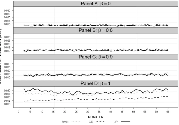
compare these indices with the official SPAR index for Waitakere City. The Waitakere City repeat-sales data, described in Grimes and Young (2010), is recorded quarterly from 1993q3 to 2009q3. The three estimated repeat-sales equations and the four house price indices (including the official SPAR index) are reported in the Appendix 1 (Tables A1.1 and A1.2, respectively). Figure 1 provides a comparison of the four indices, normalised to one in 2009q3.

The three repeat-sales methods track each other closely; the SPAR index is also very similar, albeit with a slightly greater degree of variation from the other measures.4

While the three repeat-sales price indices provide similar results in this case, we cannot rank them because we do not know the true underlying DGP. Nor can we tell whether some

Thus, the method proposed by Borassa et al does appear to provide a close approximation to a repeat-sales index. By contrast, as demonstrated in Appendix 2, simple mean and median sale price indices provide poor approximations, even after application of smoothing algorithms.

4 _{The SPAR index is calculated using data on all sales in the city whereas the repeat-sales indices rely on a random}

sample of houses (approximately 500 per quarter); one possible cause of deviation between the SPAR and repeat-sales measures is different underlying data.

Figure 1: Comparison of House Price Indices

repeat-sales methods out-perform others with alternative DGPs. In order to understand how the three repeat-sales methods compare with each other in terms of accuracy, the next section uses simulated data as a basis for estimating each of the three indices, enabling a ranking of these methods against the true data properties.

4.2.

Simulated data

Our approach compares the accuracy of the BMN, CS, and UP methods under different DGPs for εit.5

5 _{The Jansen et al method was also analysed, but its results were generally very similar to the CS method and so are}

not reported.

We do so since different time series properties of the residuals may be better handled by different repeat-sales methods. Before comparing the methods, a “true” underlying index series is generated. Our index values, corresponding to the μt in (3), are chosen so as to

replicate the average of the repeat-sales indices estimated for the Waitakere City data, but the results in no way hinge on these specific μt values; rather, it is the DGPs for εit that are crucial.

quarters. We apply a unique fixed-effect, αi, to each house, which is constant over time, but

varies across houses. These fixed-effects are uniformly distributed on (-0.1, 0.1) with mean zero. Each house has a residual, εit, that can be represented as follows:

it it

it βε φ

ε = ₋1+ (4)

where εi0 = φi0and φit ~ N(0, σ2)

We specifically consider three types of DGP:

i. β = 0, which implies that lnHPit – μt has serially uncorrelated residuals.

ii. 0 < β < 1, which implies that lnHPit – μt is mean-reverting (stationary), but

auto-correlated.

iii. β = 1, which implies that lnHPit – μt follows a random walk.

For ii, we choose a range of β values, but only present results for β = 0.8 and β = 0.9. Values of β< 0.8 produce results that are very similar to β = 0 and hence are not reported. For a given σ2_{, we then form a house price series for each house according to (3) and (4), with 100} replications for each house for each of the four values of β.6

The Grimes and Young (2010) repeat-sales data has an average of approximately 3.25 sales per house over their 65 quarter period. This equates, in any quarter, to a probability of sale of 0.05. To simulate this outcome, for each house we generate a series of 65 random numbers uniformly distributed on (0, 1) and flag any value that is less than 0.05. The flagged values represent the quarters in which a sale is deemed to occur; all other quarters have no sale for that house.

We employ each of the three methods to estimate repeat-sales indices using each of the 100 “observed” series. For a given β and σ2_{, we therefore obtain 100 estimated indices for each}

method. To compare the accuracy of each method, we compute two measures; one based on the difference between the estimated indices and the true aggregate index values across the whole time period, and one that analyses the coefficient of variation (COV) of each method for each individual quarter.

To calculate the first measure, denote the true index value for quarter t as * t I ; the estimated index value using estimation method k (k∈BMN, CS, UP) for sample j (j=1, …, 100) as jk

t

I ; and the difference between them as Dtjk(= jk t

I -It*). This measure concentrates on accuracy of the index over all observations, using the standard error of each difference series.

6

Denote the standard error of difference series jk t

D (over t=1, …, T) as D_sejk. We take the mean of jk

se

D over j=1, …, 100, denoted Dmsek ; a low value for k mse

D indicates that the index construction method on average closely replicates the true index over the full sample period.

Our second measure, k

t

COV , is defined as the ratio of the standard error across the 100 estimated indices for method k in quarter t to *

t

I . Smaller values of COVtkindicate smaller dispersion around the true index in quarter t for estimation method k. In addition, analysing

k t

COV over t enables us to observe how the dispersion of estimates changes for each k over time.

Table 1 presents the results for k mse

D for each method k, using two values for σ2: 0.01 and 0.05. For β = 0, σ2 _{= 0.05 implies that approximately one-third of house sales deviate by at} least 5% from their average value relative to the region-wide index, which seems intuitively broadly plausible. For β = 1, σ2 _{= 0.05 implies that one-third of relative house values change} permanently by at least 5% per quarter, which intuitively appears to represent a considerable over-estimate of relative house price variability over time. In interpreting our results for β = 1, we therefore consider that the σ2 _{= 0.01 results are more realistic than those using σ}2 _{= 0.05.} The results for the simulation described above, which we denote as “Case 1”, are found in Panel A of Table 1. We observe that as σ2 _increases, k

mse

D increases for all methods. This result is expected, given that σ2 _{represents the variance of the innovation, φ}

it. Also, as expected, when β

increases from 0 to 1, k mse

D increases for all k and σ2_.

A key result is that for β less than approximately 0.9, UP mse

D is smaller than the other methods, implying that the UP method is a better index estimator over all observations for a DGP that does not follow a (near) unit root. Once β approaches one (i.e. a random walk), the CS method becomes superior. This latter result reflects the benefits of the weighted estimation procedures of the CS method in dealing with a unit root process relative to the BMN or UP methods. In the presence of a random walk, the UP method is the least accurate of the methods.

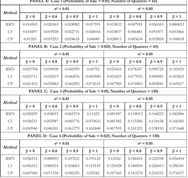
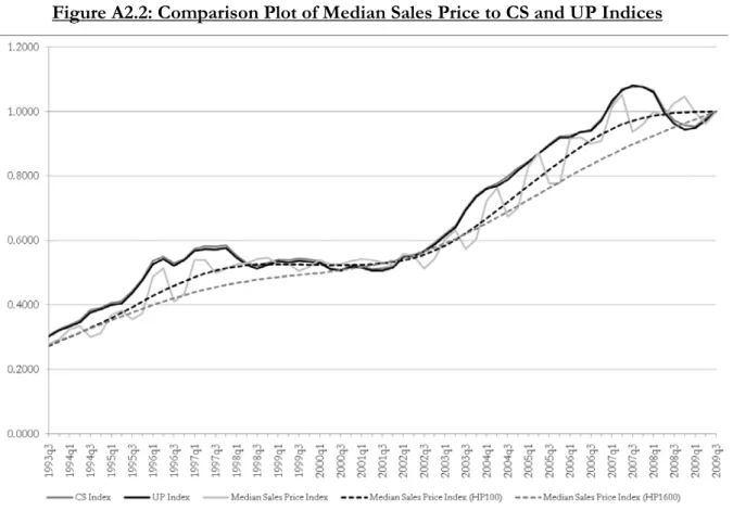
Our second measure produces results consistent with those of our first measure. Figure 2 depicts the Case 1 COV measures for all three methods when σ2_{=0.01; the four panels represent}

the four different β values.7 k

mse D

As was the case with , the magnitudes of the COV measures

across all methods increase as the value of β increases. Again, the UP method performs

Table 1: Repeat-Sales Indices Difference Measure

PANEL A: Case 1 (Probability of Sale = 0.05; Number of Quarters = 65) s Method σ2 = 0.01 σ2 = 0.05 β = 0 β = 0.8 β = 0.9 β = 1 β = 0 β = 0.8 β = 0.9 β = 1 BMN 0.014503 0.020563 0.024982 0.037591 0.033832 0.047931 0.056363 0.080652 CS 0.014497 0.019928 0.022731 0.026016 0.033837 0.046481 0.051871 0.053466 UP 0.01265 0.019253 0.024618 0.04449 0.028815 0.043634 0.055824 0.100618

PANEL B: Case 2 (Probability of Sale = 0.025; Number of Quarters = 65)

Method σ2 = 0.01 σ2 = 0.05

β = 0 β = 0.8 β = 0.9 β = 1 β = 0 β = 0.8 β = 0.9 β = 1

BMN 0.023704 0.034938 0.042959 0.06792 0.053416 0.078357 0.094728 0.155023

CS 0.023711 0.034219 0.040476 0.043949 0.053425 0.077055 0.089081 0.103823

UP 0.021452 0.032882 0.042493 0.074533 0.047985 0.074963 0.092841 0.169217

PANEL C: Case 3 (Probability of Sale = 0.05; Number of Quarters = 130)

Method σ2 = 0.01 σ2 = 0.05

β = 0 β = 0.8 β = 0.9 β = 1 β = 0 β = 0.8 β = 0.9 β = 1

BMN 0.038209 0.054015 0.065574 0.11225 0.081587 0.118012 0.144223 0.242406

CS 0.038231 0.052987 0.060776 0.070433 0.081582 0.115385 0.131638 0.166585

UP 0.030946 0.046301 0.061279 0.162448 0.067595 0.101325 0.138193 0.371648

PANEL D: Case 4 (Probability of Sale = 0.025; Number of Quarters = 130)

Method σ2 = 0.01 σ2 = 0.05

β = 0 β = 0.8 β = 0.9 β = 1 β = 0 β = 0.8 β = 0.9 β = 1

BMN 0.056512 0.080833 0.107652 0.195125 0.12542 0.186416 0.232108 0.456434

CS 0.056512 0.080214 0.104063 0.119159 0.125428 0.184954 0.224413 0.296341

UP 0.047686 0.071234 0.096335 0.25342 0.107345 0.163274 0.218331 0.576537

marginally better than the other methods for β values less than approximately 0.9. Once β reaches 0.9 (Figure 2 Panel C), the UP method loses its advantage over other methods and, in the presence of a random walk (Figure 2 Panel D), becomes the least accurate house price index. The CS method becomes the most accurate index when residuals follow a random walk.

The temporal behaviour of the COV measures for all methods is stable for stationary series. There is some evidence that sample length has an effect when β=1, with all measures rising towards the end of the time period, suggesting the deviation of estimates around the mean widens as time passes.

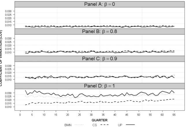
Further to Case 1 above, we test the robustness of the results against changes to two parameters: the average probability of sale and the length of the sample period. Firstly, we test a lower probability of sale for each house. The probability of sale is halved to 0.025 and we denote this as Case 2. Intuitively, fewer sales may decrease any advantage of the UP method over the

Figure 2: Case 1 COV Measures (σ2_=0.01)8

other two methods since there will be fewer occurrences when more than two sales are observed for a single house. Table 1 Panel B contains the k

mse

D measures for each method k, while Figure 3 depicts the COV measures for Case 2.

Results for Case 2 parallel those for Case 1. The UP method remains the most accurate method for β < 0.9, but surrenders this advantage once the DGP approaches a random walk, with the CS method preferable in the presence of a random walk. The effect of reducing sales numbers causes each method’s overall accuracy to drop. This result is expected since with a probability of sale of 0.025, houses sell, on average, only 1.63 times over the 65 quarters, leading to fewer sale observations per quarter from which to estimate an index.

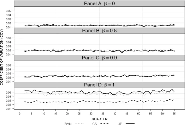
The second adjustment is to double the sample length from 65 to 130 periods, whilst keeping the probability of sale constant at 0.05 (Case 3). Comparable results (Table 1 Panel C and Figure 4) are observed for Case 3 to those in the two previous cases; however, we observe a greater drop in the overall accuracy of all methods with the longer sample length than for the

Figure 3: Case 2 COV Measures (σ2_=0.01)

reduction in average sales. With a β of 0.9, the UP method now out-performs the other methods (Figure 4), possibly due to the higher average number of sales per house and the UP method’s ability to comprehensively consider all sales of a particular house, rather than splitting them into distinct pairs. Once the DGP follows a random walk, the CS method is again superior.

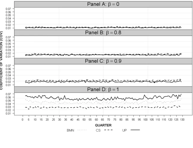
Finally, we alter both parameters by halving the probability of sale and doubling the time length to 130 periods (Case 4). Case 4 contains the same average number of sales per house as Case 1, but over a longer sample length. According to values in Table 1 Panel D, estimates of all methods are substantially less accurate than Case 1. A constant average number of sales per house over a longer period of time effectively means there are fewer sales per quarter from which to estimate the true house price index, leading to the drop in accuracy.9 _{Similar to Case 3,} the COV measures in Figure 5 show that the UP method remains more accurate than the other methods with β=0.9, suggesting the UP method is better at estimating a house price index over longer time periods provided the DGP is stationary.

Figure 5: Case 4 COV Measures (σ2_=0.01)

9

For Case 1, there are approximately 500 sales observations per quarter; comparably, Case 4 only has around 250 sales observations per quarter.

In addition to the two measures used above (Dmseand COVt), the potential for long-term bias in the estimated indices (i.e. in the growth of house prices) is an important consideration. Calculating the mean growth of the difference series (i.e. the last value less the first) for each estimation method indicates virtually zero long-term bias in any of the methods; that is, mean growth of all the difference series is approximately zero.

In-depth analysis of the properties of the different methods finds that the UP method is superior to the BMN and CS methods when relative house prices follow a stationary DGP other than one displaying a near unit root; the superiority of the UP method is magnified over longer sample periods. If relative house price shocks are (near) permanent, i.e. the residuals follow a (near) random walk, the CS method is superior due to its inherent ability to deal with

pronounced serial correlation.

5.

Conclusions

We introduce a new method for calculating a house price index using a repeat-sales approach. This new method is much simpler to compute than previously documented methods. Aside from being less demanding to compute, it is also more accurate under a wide range of conditions.

Simulations using data from differing DGPs (with relative house price innovations) are used to deduce which of the three repeat-sales methods is most accurate. Different DGPs may result in some methods being preferred to others in specific cases. This pattern is observed across the two prior methods, with the BMN and CS methods producing broadly equivalent results when house characteristics are stationary, but with the CS methodout-performing BMN when innovations to relative prices follow a non-stationary process. This result is expected given that the CS method was specifically designed to improve on BMN in such circumstances.

Comparing the two prior methods to the UP method, we find that the UP method out-performs the BMN and CS methods for stationary DGPs other than those that exhibit a near random walk.. Once residuals approach a random walk, the CS method is most accurate and the UP method becomes the least accurate. These results are robust to changes in sales numbers and time length. Additionally, we consider the potential for long-term bias in each method and find virtually no bias for any of the methods.

For a given sample of house sales, a researcher cannot know the true time series properties of the value of an individual house relative to the regional index (i.e. of εit). It is

unlikely that εit actually follows a random walk (β=1) since that would imply that an individual

house price could rise or fall indefinitely relative to its regional index. However some degree of persistence (β>0) is likely; for instance, maintenance of a house may only be carried out infrequently. In that case, the rise in value of a particular house may lag behind local area

increases for a period and then be restored to the broader regional value when the house is again fully maintained. Thus some degree of mean reversion in εit is plausible. It is then an empirical

matter whether the resulting β is greater than or less than 0.9 which we find to be the approximate cut-off value favouring the UP relative to the CS method.

In practice, the three repeat-sales methods produce very similar results to one another (and similar results to a SPAR index) when using actual data. Undoubtedly, however, the UP method is computationally the simplest of the methods to implement and so represents a new, simpler and accurate method for those wishing to estimate a mix-adjusted housing index.

References

Abraham, Jesse M. and William S. Schauman. 1991. “New evidence on home prices from Freddie Mac repeat-sales,” Journal of the American Real Estate & Urban Economics Association, 19, 333-352.

Bailey, Martin J., Richard F. Muth and Hugh O. Nourse. 1963. “A regression method for real estate price index construction,” Journal of the American Statistical Association, 58, 933-942.

Bourassa, Steven C., Martin Hoesli, and Jian Sun. 2006. “A simple alternative house price index method,” Journal of Housing Economics, 15, 80-97.

Case, Karl E. and Robert J. Shiller. 1987. “Prices of single-family homes since 1970: New indexes for four cities,” New England Economic Review, Sep, 45-56.

de Vries, Paul, Jan de Haan, Erna van der Wal and Gust Mariën. 2009. “A house price index based on the SPAR method,” Journal of Housing Economics, 18, 214-223.

Grimes, Arthur and Chris Young. 2010. “Anticipatory Effects of Rail Upgrades: Auckland’s Western Line” Motu Working Paper, Motu Economic and Public Policy Research, Wellington. Jansen, S. J. T., P. de Vries, H. C. C. H. Coolen, C. J. M. Lamain, and P.J. Boelhouwer. 2008. “Developing a house price index for The Netherlands: A practical application of weighted repeat-sales,” The Journal of Real Estate Finance and Economics, 37, 163-186.

McMillen, Daniel P. and John McDonald. 2004. “Reaction of house prices to a new rapid transit line: Chicago’s Midway Line, 1983-1999,” Real Estate Economics, 32, 463-486.

Wang, Ferdinand T. and Peter M. Zorn. 1997. “Estimating house price growth with repeat-sales data: What’s the aim of the game?” Journal of Housing Economics, 6, 93-118.

Appendix 1: House Price Index Results

Table A1.1: Regression Results for House Price Indices

BMN Index CS Index UP Index

1993q4 0.0612 0.0579 0.0639 (0.0156) (0.0160) (0.0145) 1994q1 0.100 0.0995 0.100 (0.0149) (0.0151) (0.0141) 1994q2 0.143 0.142 0.138 (0.0144) (0.0146) (0.0136) 1994q3 0.223 0.226 0.221 (0.0151) (0.0152) (0.0144) 1994q4 0.242 0.248 0.247 (0.0145) (0.0146) (0.0140) 1995q1 0.282 0.285 0.280 (0.0149) (0.0150) (0.0142) 1995q2 0.294 0.297 0.293 (0.0144) (0.0144) (0.0140) 1995q3 0.371 0.370 0.368 (0.0141) (0.0142) (0.0136) 1995q4 0.452 0.453 0.455 (0.0140) (0.0141) (0.0136) 1996q1 0.560 0.564 0.555 (0.0134) (0.0135) (0.0129) 1996q2 0.585 0.588 0.586 (0.0145) (0.0146) (0.0144) 1996q3 0.548 0.548 0.546 (0.0146) (0.0147) (0.0146) 1996q4 0.574 0.574 0.579 (0.0146) (0.0148) (0.0145) 1997q1 0.628 0.630 0.630 (0.0138) (0.0139) (0.0135) 1997q2 0.644 0.646 0.642 (0.0139) (0.0141) (0.0138) 1997q3 0.635 0.642 0.637 (0.0141) (0.0143) (0.0141) 1997q4 0.649 0.651 0.645 (0.0145) (0.0147) (0.0146) 1998q1 0.589 0.593 0.592 (0.0152) (0.0153) (0.0155) 1998q2 0.551 0.552 0.553 (0.0157) (0.0158) (0.0158) 1998q3 0.530 0.532 0.530 (0.0146) (0.0147) (0.0147) 1998q4 0.548 0.553 0.551 (0.0146) (0.0148) (0.0147) 1999q1 0.569 0.572 0.572 (0.0144) (0.0145) (0.0143) 1999q2 0.563 0.568 0.567 (0.0146) (0.0147) (0.0146) 1999q3 0.575 0.578 0.575 (0.0145) (0.0146) (0.0146) 1999q4 0.568 0.571 0.568 (0.0144) (0.0145) (0.0143) 2000q1 0.559 0.562 0.562 (0.0146) (0.0147) (0.0148) 2000q2 0.519 0.521 0.526 (0.0154) (0.0155) (0.0158) 2000q3 0.506 0.509 0.518 (0.0159) (0.0160) (0.0164) 2000q4 0.536 0.539 0.540 (0.0148) (0.0149) (0.0151) 2001q1 0.528 0.531 0.534 (0.0149) (0.0150) (0.0152) 2001q2 0.510 0.515 0.516 (0.0153) (0.0154) (0.0156) 2001q3 0.519 0.522 0.518 (0.0147) (0.0148) (0.0152) 2001q4 0.526 0.528 0.535 (0.0144) (0.0145) (0.0145) 2002q1 0.586 0.588 0.596 (0.0138) (0.0139) (0.0139) 2002q2 0.592 0.595 0.601 (0.0138) (0.0139) (0.0139)

2002q3 0.618 0.620 0.629 (0.0137) (0.0138) (0.0137) 2002q4 0.659 0.663 0.663 (0.0133) (0.0134) (0.0132) 2003q1 0.704 0.707 0.711 (0.0132) (0.0134) (0.0131) 2003q2 0.746 0.749 0.750 (0.0129) (0.0131) (0.0127) 2003q3 0.825 0.826 0.832 (0.0129) (0.0131) (0.0126) 2003q4 0.881 0.885 0.889 (0.0127) (0.0129) (0.0124) 2004q1 0.913 0.915 0.922 (0.0131) (0.0132) (0.0130) 2004q2 0.929 0.934 0.935 (0.0132) (0.0133) (0.0130) 2004q3 0.958 0.961 0.959 (0.0136) (0.0136) (0.0136) 2004q4 0.991 0.993 0.994 (0.0134) (0.0135) (0.0135) 2005q1 1.017 1.018 1.024 (0.0131) (0.0132) (0.0129) 2005q2 1.045 1.046 1.058 (0.0134) (0.0135) (0.0134) 2005q3 1.078 1.079 1.086 (0.0131) (0.0132) (0.0129) 2005q4 1.101 1.106 1.112 (0.0136) (0.0136) (0.0135) 2006q1 1.105 1.108 1.112 (0.0136) (0.0137) (0.0136) 2006q2 1.116 1.119 1.131 (0.0138) (0.0138) (0.0138) 2006q3 1.126 1.129 1.135 (0.0135) (0.0135) (0.0135) 2006q4 1.160 1.163 1.169 (0.0133) (0.0134) (0.0133) 2007q1 1.208 1.210 1.229 (0.0130) (0.0131) (0.0122) 2007q2 1.250 1.254 1.261 (0.0130) (0.0131) (0.0122) 2007q3 1.259 1.260 1.275 (0.0129) (0.0131) (0.0121) 2007q4 1.258 1.261 1.271 (0.0130) (0.0132) (0.0121) 2008q1 1.245 1.248 1.255 (0.0131) (0.0134) (0.0122) 2008q2 1.190 1.194 1.195 (0.0133) (0.0136) (0.0125) 2008q3 1.155 1.158 1.158 (0.0134) (0.0136) (0.0125) 2008q4 1.137 1.143 1.139 (0.0136) (0.0140) (0.0127) 2009q1 1.133 1.138 1.145 (0.0131) (0.0135) (0.0122) 2009q2 1.162 1.165 1.169 (0.0131) (0.0135) (0.0122) 2009q3 1.182 1.186 1.197 (0.0131) (0.0135) (0.0122) Observations 10516 10516 16245 R-squared 0.893 0.877 0.922 Number of houses 5729 5729 5729

Quarter

Table A1.2: House Price Indices

BMN Index CS Index UP Index SPAR Index 1993q3 0.3067 0.3054 0.3021 0.2990 1993q4 0.3260 0.3236 0.3220 0.3154 1994q1 0.3389 0.3374 0.3339 0.3278 1994q2 0.3538 0.3520 0.3468 0.3470 1994q3 0.3833 0.3829 0.3768 0.3678 1994q4 0.3906 0.3914 0.3867 0.3892 1995q1 0.4066 0.4062 0.3997 0.3950 1995q2 0.4115 0.4111 0.4049 0.4023 1995q3 0.4444 0.4422 0.4365 0.4318 1995q4 0.4819 0.4805 0.4762 0.4689 1996q1 0.5369 0.5369 0.5262 0.5114 1996q2 0.5505 0.5499 0.5428 0.5328 1996q3 0.5305 0.5283 0.5215 0.5293 1996q4 0.5444 0.5423 0.5390 0.5383 1997q1 0.5746 0.5735 0.5672 0.5524 1997q2 0.5839 0.5827 0.5741 0.5603 1997q3 0.5787 0.5804 0.5712 0.5584 1997q4 0.5868 0.5857 0.5758 0.5517 1998q1 0.5527 0.5527 0.5461 0.5424 1998q2 0.5321 0.5305 0.5252 0.5137 1998q3 0.5210 0.5200 0.5132 0.5050 1998q4 0.5305 0.5310 0.5241 0.5210 1999q1 0.5417 0.5412 0.5353 0.5248 1999q2 0.5385 0.5390 0.5326 0.5236 1999q3 0.5450 0.5444 0.5369 0.5280 1999q4 0.5412 0.5406 0.5331 0.5261 2000q1 0.5363 0.5358 0.5299 0.5223 2000q2 0.5153 0.5143 0.5112 0.5047 2000q3 0.5086 0.5081 0.5071 0.5053 2000q4 0.5241 0.5236 0.5184 0.5079 2001q1 0.5200 0.5194 0.5153 0.5101 2001q2 0.5107 0.5112 0.5061 0.5044 2001q3 0.5153 0.5148 0.5071 0.5111 2001q4 0.5189 0.5179 0.5158 0.5268 2002q1 0.5510 0.5499 0.5483 0.5389 2002q2 0.5543 0.5538 0.5510 0.5504 2002q3 0.5689 0.5678 0.5667 0.5581 2002q4 0.5927 0.5927 0.5863 0.5783 2003q1 0.6200 0.6194 0.6151 0.6029 2003q2 0.6466 0.6460 0.6395 0.6166 2003q3 0.6998 0.6977 0.6942 0.6844 2003q4 0.7401 0.7401 0.7349 0.7199 2004q1 0.7641 0.7626 0.7596 0.7503 2004q2 0.7765 0.7772 0.7695 0.7686 2004q3 0.7993 0.7985 0.7882 0.7865 2004q4 0.8261 0.8245 0.8163 0.8029 2005q1 0.8479 0.8454 0.8411 0.8321 2005q2 0.8720 0.8694 0.8702 0.8547 2005q3 0.9012 0.8985 0.8949 0.8817 2005q4 0.9222 0.9231 0.9185 0.9041 2006q1 0.9259 0.9250 0.9185 0.9233 2006q2 0.9361 0.9352 0.9361 0.9245 2006q3 0.9455 0.9446 0.9399 0.9410 2006q4 0.9782 0.9773 0.9724 0.9741 2007q1 1.0263 1.0243 1.0325 1.0216 2007q2 1.0704 1.0704 1.0661 1.0540 2007q3 1.0800 1.0768 1.0811 1.0626 2007q4 1.0790 1.0779 1.0768 1.0677 2008q1 1.0650 1.0640 1.0597 1.0562 2008q2 1.0080 1.0080 0.9980 1.0072 2008q3 0.9734 0.9724 0.9618 0.9748 2008q4 0.9560 0.9579 0.9436 0.9618 2009q1 0.9522 0.9531 0.9493 0.9626 2009q2 0.9802 0.9792 0.9724 0.9705 2009q3 1.0000 1.0000 1.0000 1.0000

Appendix 2: Mean and Median Sales Price Comparison

We compare the raw mean and median sales prices in Waitakere City, with the CS and UP indices over the same time period. The raw series contain significant quarter to quarter fluctuation. To smooth the series, HP filters are applied with two different smoothing parameters, 1600 (often used to extract cycles from quarterly data) and 100. All series are normalised to one in 2009q3 and the trends from 1993q3 to 2009q3 are plotted, along with the CS and UP indices. The mean sales price series are seen in Figure A2.1, and the median sales price series in Figure A2.2. The mean and median price trends broadly follow the CS and UP indices; however, they fluctuate much more on a quarterly basis and are generally lower than the CS and UP indices. This latter feature implies that the raw (mean and median) series overstate house price appreciation over the full time period. The HP filtered series with smoothing parameter 100 are the closer of the two HP filtered series to the CS and UP indices.

Figure A2.1: Comparison Plot of Mean Sales Price, CS and UP Indices

Appendix 3: COV Measures for σ

_=0.05

Figure A3.1: Case 1 COV Measures

Figure A3.3: Case 3 COV Measures

Recent Motu Working Papers

All papers in the Motu Working Paper Series are available on our website www.motu.org.nz, or by

contacting us o

10-09 Evans, Lewis; Greame Guthrie and Andrea Lu. 2010. "A New Zealand Electricity Market Model: Assessment of the Effect of Climate Change on Electricity Production and Consumption".

10-08 Coleman, Andrew and Hugh McDonald. 2010. "“No country for old men”: a note on the trans-Tasman income divide".

10-07 Grimes, Arthur; Mark Holmes and Nicholas Tarrant. 2010. "New Zealand Housing Markets: Just a Bit-Player in the A-League?"

10-06 Le, Trinh; John Gibson and Steven Stillman. 2010. "Household Wealth and Saving in New Zealand: Evidence from the Longitudinal Survey of Family, Income and Employment".

10-05 Grimes, Arthur. 2010. "The Economics of Infrastructure Investment: Beyond Simple Cost Benefit Analysis".

10-04 van Benthem, Arthur and Suzi Kerr. 2010. “Optimizing Voluntary Deforestation Policy in the Face of Adverse Selection and Costly Transfers”.

10-03 Roskruge, Matthew; Arthur Grimes; Philip McCann and Jacques Poot. 2010. "Social Capital and Regional Social Infrastructure Investment: Evidence from New Zealand”.

10-02 Coleman, Andrew. 2010. "Uncovering uncovered interest parity during the classical gold standard era, 1888-1905".

10-01 Coleman, Andrew. 2010. "Squeezed in and squeezed out: the effects of population ageing on the demand for housing".

09-17 Todd, Maribeth and Suzi Kerr. 2009. "How Does Changing Land Cover and Land Use in New Zealand relate to Land Use Capability and Slope?"

09-16 Kerr, Suzi and Wei Zhang. 2009. "Allocation of New Zealand Units within Agriculture in the New Zealand Emissions Trading System”.

09-15 Grimes, Arthur; Cleo Ren and Philip Stevens. 2009. "The Need for Speed: Impacts of Internet Connectivity on Firm Productivity”.

09-14 Coleman, Andrew and Arthur Grimes. 2009. "Fiscal, Distributional and Efficiency Impacts of Land and Property Taxes”.

09-13 Coleman, Andrew. 2009. "The Long Term Effects of Capital Gains Taxes in New Zealand”.

09-12 Grimes, Arthur and Chris Young. 2009. "Spatial Effects of 'Mill' Closure: Does Distance Matter?"

09-11 Maré, David C and Steven Stillman. 2009. "The Impact of Immigration on the Labour Market Outcomes of New Zealanders”.

09-10 Stillman, Steven and David C Maré. 2009. "The Labour Market Adjustment of Immigrants in New Zealand”.

09-09 Kerr, Suzi and Kelly Lock. 2009. “Nutrient Trading in Lake Rotorua: Cost Sharing and Allowance Allocation”.