Object-Oriented Type Inference

(1)

Object-Oriented Type Inference

Jens Palsberg and Michael I. Schwartzbach

Computer Science Department, Aarhus University Ny Munkegade, DK-8000 ˚Arhus C, Denmark

Abstract

We present a new approach to inferring types in un-typed object-oriented programs with inheritance, assignments, and late binding. It guarantees that all messages are understood, annotates the pro-gram with type information, allows polymorphic methods, and can be used as the basis of an op-timizing compiler. Types are finite sets of classes and subtyping is set inclusion. Using atrace graph, our algorithm constructs a set of conditional type constraints and computes the least solution by least fixed-point derivation.

1 Introduction

Untyped object-oriented languages with assign-ments and late binding allow rapid prototyping be-cause classes inherit implementation and not spec-ification. Late binding, however, can cause pro-grams to be unreliable, unreadable, and inefficient [27]. Type inference may help solve these prob-lems, but so far no proposed inference algorithm has been capable of checking most common, com-pletely untyped programs [9].

We present a new type inference algorithm for a basic object-oriented language with inheritance, as-signments, and late binding.

In Proc. ACM Conference on Object-Oriented Programming: Systems, Languages, and Applications (OOPSLA) October 6-11, 1991, pages 146–161.

c

1991 ACM. Copied by permission.

The algorithm guarantees that all messages are un-derstood, annotates the program with type infor-mation, allows polymorphic methods, and can be used as the basis of an optimizing compiler. Types are finite sets of classes and subtyping is set in-clusion. Given a concrete program, the algorithm constructs a finite graph of type constraints. The program istypable if these constraints are solvable. The algorithm then computes the least solution in worst-case exponential time. The graph contains all type information that can be derived from the program without keeping track ofnilvalues or flow analyzing the contents of instance variables. This makes the algorithm capable of checking most com-mon programs; in particular, it allows for polymor-phic methods. The algorithm is similar to previous work on type inference [18, 14, 27, 1, 2, 19, 12, 10, 9] in using type constraints, but it differs in handling late binding by conditional constraints and in re-solving the constraints by least fixed-point deriva-tion rather than unificaderiva-tion.

The example language resembles Smalltalk [8] but avoids metaclasses, blocks, and primitive meth-ods. Instead, it provides explicit new and if-then-else expressions; classes like Natural can be pro-grammed in the language itself.

In the following section we discuss the impacts of late binding on type inference and examine previ-ous work. In later sections we briefly outline the example language, present the type inference algo-rithm, and show some examples of its capabilities.

(2)

2 Late Binding

Late binding means that a message send is dynam-ically bound to an implementation depending on the class of the receiver. This allows a form of poly-morphism which is fundamental in object-oriented programming. It also, however, involves the danger that the class of the receiver doesnot implement a method for the message—the receiver may even be nil. Furthermore, late binding can make the control flow of a program hard to follow and may cause a time-consuming run-time search for an implemen-tation.

It would significantly help an optimizing compiler if, for each message send in a program text, it could infer the following information.

• Can the receiver be nil?

• Can the receiver be an instance of a class which does not implement a method for the message? • What are the classes of all possible non-nil

re-ceivers in any execution of the program? Note that the available set of classes is induced by the particular program. These observations lead us to the following terminology.

Terminology:

Type: A type is a finite set of classes.

Induced Type: The induced type of an ex-pression in a concrete program is the set of classes of all possible non-nil values to which it may evaluate in any execution of that particular program.

Sound approximation: A sound approxima-tion of the induced type of an expression in a concrete program is a superset of the induced type.

Note that a sound approximation tells “the whole truth”, but not always “nothing but the truth” about an induced type. Since induced types are

generally uncomputable, a compiler must make do with sound approximations. An induced type is a subtype of any sound approximation; subtyp-ing is set inclusion. Note also that our notion of type, which we also investigated in [22], differs from those usually used in theoretical studies of types in object-oriented programming [3, 7]; these theories have difficulties with late binding and assignments. The goals of type inference can now be phrased as follows.

Goals of type inference:

Safety guarantee: A guarantee that any mes-sage is sent to either nil or an instance of a class which implements a method for the message; and, given that, also

Type information: A sound approximation of the induced type of any receiver.

Note that we ignore checking whether the receiver isnil; this is a standard data flow analysis problem which can be treated separately.

If a type inference is successful, then the program istypable; the errormessageNotUnderstood will not occur. A compiler can use this to avoid inserting some checks in the code. Furthermore, if the type information of a receiver is a singleton set, then the compiler can do early binding of the message to the only possible method; it can even do in-line substitution. Similarly, if the type information is anempty set, then the receiver is known to always be nil. Finally, type information obtained about variables and arguments may be used to annotate the program for the benefit of the programmer.

Smalltalkand other untyped object-oriented lan-guages are traditionally implemented by interpret-ers. This is ideal for prototyping and exploratory development but often too inefficient and space de-manding for real-time applications and embedded systems. What is needed is an optimizing compiler that can be used near the end of the programming phase, to get the required efficiency and a safety guarantee. A compiler which produces good code

(3)

can be tolerated even it is slow because it will be used much less often than the usual programming environment. Our type inference algorithm can be used as the basis of such an optimizing com-piler. Note, though, that both the safety guaran-tee and the induced types are sensitive to small changes in the program. Hence, separate compi-lation of classes seems impossible. Typed object-oriented languages such as Simula[6]/Beta [15],

C++[26], andEiffel[17] allow separate compila-tion but sacrifice flexibility. The relacompila-tions between types and implementation are summarized in fig-ure 1.

When programs are: Their implementation is:

Untyped Interpretation

Typable Compilation

Typed Separate Compilation

Figure 1: Types and implementation. Graver and Johnson [10, 9], in their type system forSmalltalk_{, take an intermediate approach}

be-tween “untyped” and “typed” in requiring the pro-grammer to specify types for instance variables whereas types of arguments are inferred. Suzuki [27], in his pioneering work on inferring types in

Smalltalk, handles late binding by assuming that each message send may invoke all methods for that message. It turned out, however, that this yields an algorithm which is not capable of checking most common programs.

Both these approaches include a notion of method type. Our new type inference algorithm abandons this idea and uses instead the concept ofconditional constraints, derived from a finite graph. Recently, Hense [11] addressed type inference for a language

O’Smallwhich is almost identical to our example language. He uses a radically different technique, with type schemes and unification based on work of R´emy [24] and Wand [29]. His paper lists four pro-grams of which his algorithm can type-check only the first three. Our algorithm can type-check all

four, in particular the fourth which is shown in figure 11 in appendix B. Hense uses record types which can be extendible and recursive. This seems to produce less precise typings than our approach, and it is not clear whether the typings would be useful in an optimizing compiler. One problem is that type schemes always correspond to either sin-gletons or infinite sets of monotypes; our finite sets can be more precise. Hense’s and ours approaches are similar in neither keeping track of nil values nor flow analyzing the contents of variables. We are currently investigating other possible relations. Before going into the details of our type inference algorithm we first outline an example language on which to apply it.

3 The Language

Our example language resembles Smalltalk_{, see}

figure 2.

Aprogram is a set of classes followed by an expres-sion whose value is the result of executing the pro-gram. Aclass can be defined using inheritance and contains instance variables and methods; amethod is a message selector (m1 . . . mn ) with formal

pa-rameters and an expression. The language avoids metaclasses, blocks, and primitive methods. In-stead, it provides explicit new and if-then-else ex-pressions (the latter tests if the condition is non-nil). The result of a sequence is the result of the last expression in that sequence. The expression “self class new” yields an instance of the class of self. The expression “E instanceOf ClassId” yields a run-time check for class membership. If the check fails, then the expression evaluates to nil.

The Smalltalk system is based on some primi-tive methods, written in assembly language. This dependency on primitives is not necessary, at least not in this theoretical study, because classes such asTrue,False,Natural, andListcan be programmed in the language itself, as shown in appendix A.

(4)

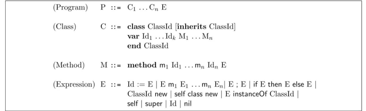
(Program) P ::= C1 . . . Cn E

(Class) C ::= class ClassId [inherits ClassId] varId1 . . . Idk M1 . . . Mn

end ClassId

(Method) M::= method m1 Id1 . . .mn Idn E

(Expression) E ::= Id:= E | Em1 E1 . . .mn En| E; E | ifE thenE elseE |

Figure 2: Syntax of the example language.

4 Type Inference

Our type inference algorithm is based on three fun-damental observations.

Observations:

Inheritance: Classes inherit implementation and not specification.

Classes: There are finitely many classes in a program.

Message sends: There are finitely many syn-tactic message sends in a program.

The first observation leads to separate type infer-ence for a class and its subclasses. Notionally, this is achieved by expanding all classes before doing type inference. This expansion means removing all inheritance by

• Copying the text of a class to its subclasses • Replacing each message send to super by a

message send to a renamed version of the in-herited method

• Replacing each “self class new” expression by a “ClassIdnew” expression where ClassId is the enclosing class in the expanded program. This idea of expansion is inspired by Graver and Johnson [10, 9]; note that the size of the expanded

program is at most quadratic in the size of the orig-inal.

The second and third observation lead to a finite representation of type information about all execu-tions of the expanded program; this representation is called the trace graph. From this graph a finite set of type constraints will be generated. Typa-bility of the program is then solvaTypa-bility of these constraints. Appendix B contains seven example programs which illustrate different aspects of the type inference algorithm, see the overview in fig-ure 3. The program texts are listed together with the corresponding constraints and their least solu-tion, if it exists. Hense’s program in figure 11 is the one he gives as a typical example of what he cannot type-check [11]. We invite the reader to consult the appendix while reading this section.

A trace graph contains three kinds of type infor-mation.

Three kinds of type information:

Local constraints: Generated from method bodies; contained in nodes.

Connecting constraints: Reflect message sends; attached to edges.

Conditions: Discriminate receivers; attached to edges.

(5)

Example program in: Illustrates: Can we type it?

Figure 10 Basic type inference Yes

Figure 11 Hense’s program Yes

Figure 12 A polymorphic method Yes

Figure 13 A recursive method Yes

Figure 14 Lack of flow analysis No

Figure 15 Lack of nildetection No

Figure 16 A realistic program Yes

Figure 3: An overview of the example programs.

4.1 Trace Graph Nodes

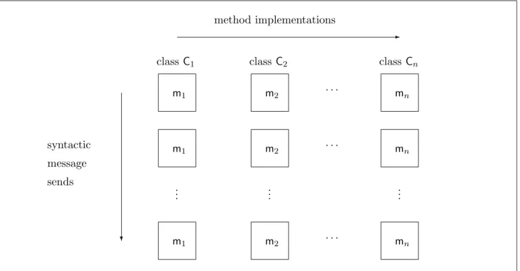
The nodes of the trace graph are obtained from the various methods implemented in the program. Each method yields a number of different nodes: one for each syntactic message send with the cor-responding selector. The situation is illustrated in figure 4, where we see the nodes for a method m that is implemented in each of the classes C1,C2,. . . ,Cn. Thus, the number of nodes in the

trace graph will at most be quadratic in the size of the program. There is also a single node for the main expression of the program, which we may think of as a special method without parameters. Methods do not have types, but they can be pro-vided with type annotations, based on the types of their formal parameters and result. A particu-lar method implementation may be represented by several nodes in the trace graph. This enables it to be assigned several different type annotations—one for each syntactic call. This allows us effectively to obtain method polymorphism through a finite set of method “monotypes”.

4.2 Local Constraints

Each node contains a collection oflocal constraints that the types of expressions must satisfy. For each syntactic occurrence of an expression E in the im-plementation of the method, we regard its type as

an unknown variable [[E]]. Exact type information is, of course, uncomputable. In our approach, we will ignore the following two aspects of program ex-ecutions.

Approximations:

Nil values: It does not keep track ofnilvalues. Instance variables: It does not flow analyze

the contents of instance variables.

The first approximation stems from our discussion of the goals of type inference; the second corre-sponds to viewing an instance variable as having a single possibly large type, thus leading us to iden-tify the type variables of different occurrences of the same instance variable. In figures 14 and 15 we present two program fragments that are typical for what we cannot type because of these approxi-mations. In both cases the constraints demand the false inclusion{True} ⊆ {Natural}. Suzuki [27] and Hense [11] make the same approximations.

For an expression E, the local constraints are gener-ated from all the phrases in its derivation, accord-ing to the rules in figure 5. The idea of generat-ing constraints on type variables from the program syntax is also exploited in [28, 25].

The constraints guarantee safety; only in the cases 4) and 8) do the approximations manifest them-selves. Notice that the constraints can all be

(6)

ex-? -.. . .. . .. . · · · · · · · · · sends message syntactic method implementations m2 m1 m1 m2 mn mn mn m2 m1 classCn classC2 classC1

Figure 4: Trace graph nodes. pressed as inequalities of one of the three forms:

“constant ⊆ variable”, “variable ⊆ constant”, or “variable⊆variable”; this will be exploited later. Each different node employs unique type variables, except that the types of instance variables are com-mon to all nodes corresponding to methods imple-mented in the same class. A similar idea is used by Graver and Johnson [10, 9].

4.3 Trace Graph Edges

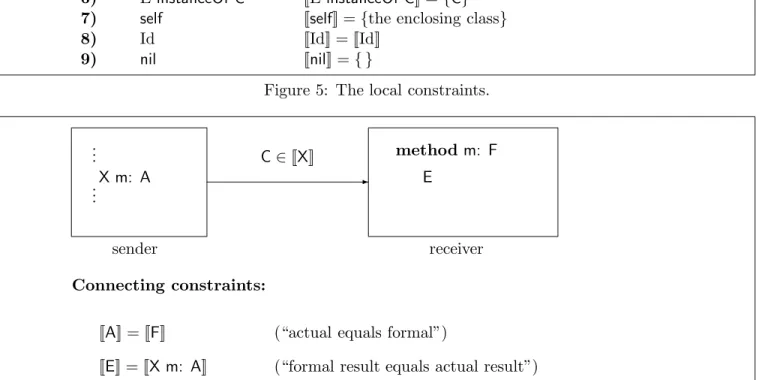
Theedgesof the trace graph will reflect the possible connections between a message send and a method that may implement it. The situation is illustrated in figure 6.

If a node corresponds to a method which contains a message send of the formX m: A, then we have an edge from that sender node to any other receiver node which corresponds to an implementation of a method m. We label this edge with the condition that the message send may be executed, namely C∈[[X]] whereCis the class in which the particular

methodmis implemented. With the edge we asso-ciate the connecting constraints, which reflect the relationship between formal and actual parameters and results. This situation generalizes trivially to methods with several parameters. Note that the number of edges is again quadratic in the size of the program.

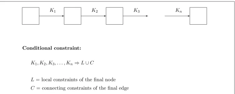
4.4 Global Constraints

To obtain the global constraints for the entire pro-gram we combine local and connecting constraints in the manner illustrated in figure 7. This pro-duces conditional constraints, where the inequali-ties need only hold if all the conditions hold. The global constraints are simply the union of the con-ditional constraints generated by all paths in the graph, originating in the node corresponding to the main expression of the program. This is a finite set, because the graph is finite; as shown later in this section, the size of the constraint set may in (ex-treme) worst-cases become exponential.

(7)

Expression: Constraint:

1) Id:= E [[Id]]⊇[[E]] ∧ [[Id:= E]] = [[E]] 2) Em1 E1 . . .mn En [[E]]⊆ {C|C implements m1. . .mn}

3) E1 ; E2 [[E1 ; E2]] = [[E2]]

4) ifE1 thenE2 elseE3 [[ifE1 thenE2 elseE3]]⊇[[E2]]∪[[E3]]

5) C new [[C new]] ={C}

6) EinstanceOf C [[E instanceOf C]] ={C} 7) self [[self]] ={the enclosing class}

8) Id [[Id]] = [[Id]]

9) nil [[nil]] ={ }

Figure 5: The local constraints.

-sender receiver

(“formal result equals actual result”) (“actual equals formal”)

[[E]] = [[X m: A]] [[A]] = [[F]] Connecting constraints: C∈[[X]] E method m: F .. . X m: A .. .

Figure 6: Trace graph edges. this provides approximate information about the

dynamic behavior of the program.

Consider any execution of the program. While ob-serving this, we can trace the pattern of method executions in the trace graph. Let E be some ex-pression that is evaluated at some point, letval(E) be its value, and let class(b) be the class of an object b. If L is some solution to the global con-straints, then the following result holds.

Soundness Theorem:

If val(E)6=nil thenclass(val(E))∈L([[E]]) It is quite easy to see that this must be true. We sketch a proof by induction in the number of mes-sage sends performed during the trace. If this is zero, then we rely on the local constraints alone;

given a dynamic semantics [4, 5, 23, 13] one can eas-ily verify that their satisfaction implies the above property. If we extend a trace with a message send X m: A implemented by a method in a class C, then we can inductively assume that C ∈ L([[X]]). But this implies that the local constraints in the node corresponding to the invoked method must hold, since all their conditions now hold and L is a solution. Since the relationship between actual and formal parameters and results is soundly rep-resented by the connecting constraints, which also must hold, the result follows.

Note that an expression E occurring in a method that appears k times in the trace graph has k type variables [[E]]1,[[E]]2, . . . ,[[E]]k in the global

(8)

-C = connecting constraints of the final edge L= local constraints of the final node K1, K2, K3, . . . , Kn⇒L∪C Conditional constraint: Kn K3 K2 K1

Figure 7: Conditional constraints from a path. type of E is obtained as

[ i

L([[E]]i)

Appendix C gives an efficient algorithm to compute the smallest solution of the extracted constraints, or to decide that none exists. The algorithm is at worst quadratic in the size of the constraint set. The complete type inference algorithm is summa-rized in figure 8.

4.5 Type Annotations

Finally, we will consider how a solution L of the type constraints can produce a type annotation of the program. Such annotations could be provided for the benefit of the programmer.

An instance variable x has only a single associ-ated type variable. The type annotation is sim-ply L([[x]]). The programmer then knows an upper bound of the set of classes whose instances may reside inx.

A method has finitely many type annotations, each of which is obtained from a corresponding node in the trace graph. If the method, implemented in the classC, is

Input: A program in the example language. Output: Either: a safety guarantee and type

information about all expressions; or: “un-able to type the program”.

1) Expand all classes.

2) Construct the trace graph of the expanded program.

3) Extract a set of type constraints from the trace graph.

4) Compute the least solution of the set of type constraints. If such a solution exists, then output it as the wanted type information, together with a safety guarantee; otherwise, output “unable to type the program”. Figure 8: Summary of the type inference algorithm.

method m1: F1 m2: F2 . . . mn: Fn

E

then each type annotation is of the form {C} ×L([[F1]])× · · · ×L([[Fn]])→L([[E]])

The programmer then knows the various manners in which this method may be used.

(9)

informa-tion about methods than the method types used by Suzuki. Consider for example the polymorphic identity function in figure 12. Our technique yields both of the method type annotations

id: {C} × {True} → {True} id: {C} × {Natural} → {Natural}

whereas the method type using Suzuki’s framework is

id: {C} × {True,Natural} → {True,Natural} which would allow neither the succ nor the isTrue message send, and, hence, would lead to rejection of the program.

4.6 An Exponential Worst-Case

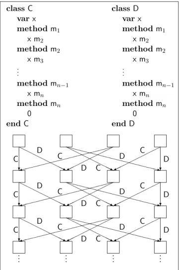
The examples in appendix B show several cases where the constraint set is quite small, in fact linear in the size of the program. While this will often be the situation, the theoretical worst-case allows the constraint set to become exponential in the size of the program. The running time of the inference algorithm depends primarily on the topology of the trace graph.

In figure 9 is shown a program and a sketch of its trace graph. The induced constraint set will be ex-ponential since the graph has exex-ponentially many different paths. Among the constraints will be a family whose conditions are similar to the words of the regular language

(CCC+DCC)n3

the size of which is clearly exponential in n. Note that this situation is similar to that of type inference in ML, which is also worst-case exponen-tial but very useful in practice. The above scenario is in fact not unlike the one presented in [16] to il-lustrate exponential running times in ML. Another similarity is that both algorithms generate a po-tentially exponential constraint set that is always solved in polynomial time.

class C class D varx var x method m1 method m1 x m2 x m2 method m2 method m2 x m3 x m3 .. . ... method mn−1 method mn−1 x mn x mn method mn method mn 0 0 endC end D ? HH HH HHHj HH HH HHHj XXXX_XXXX XXXXXz 9 ? ? 9 XXXX_XXXX XXXXXz HH HH HHHj HH HH HHHj ? ? HH HH HHHj HH HH HHHj XXXX_XXXX XXXXXz 9 ? .. . .. . .. . .. . D D D C C C C D D D D D D C C C C C C C C D D D

Figure 9: A worst-case program.

5 Conclusion

Our type inference algorithm is sound and can han-dle most common programs. It is also conceptually simple: a set of uniform type constraints is con-structed and solved by fixed-point derivation. It can be further improved by an orthogonal effort in data flow analysis.

The underlying type system is simple: types are finite sets of classes and subtyping is set inclusion. An implementation of the type inference algorithm is currently being undertaken. Future work in-cludes extending this into an optimizing compiler. The inference algorithm should be easy to modify to work for full Smalltalk, because metaclasses

(10)

are simply classes, blocks can be treated as objects with a single method, and primitive methods can be handled by stating the constraints that the ma-chine code must satisfy. Another challenge is to extend the algorithm to produce type annotations together with type substitution, see [20, 21, 22].

Appendix A: Basic classes

class Object end Object class True method isTrue Object new end True class False method isTrue nil end False

Henceforth, we abbreviate “True new” as “true”, and “Falsenew” as “false”.

class Natural varrep

method isZero

ifrep thenfalse elsetrue method succ

(Natural new) update: self method update: x

rep := x; self method pred

if(self isZero) isTrue thenself elserep method less: i

if(i isZero) isTrue thenfalse

else if (self isZero) isTruethen true else(self pred) less: (i pred)

end Natural

Henceforth, we abbreviate “Natural new” as “0”, and, recursively, “nsucc” as “n+ 1”.

class List

var head, tail

method setHead: h setTail: t head := h; tail := t

method cons: x

(self class new) setHead: x setTail: self method isEmpty

ifhead thenfalse elsetrue method car

head method cdr

tail

method append: aList if(self isEmpty) isTrue thenaList

else(tail append: aList) cons: head method insert: x

if(self isEmpty) isTrue thenself cons: x else

if(head less: x) isTrue thenself cons: x

else(tail insert: x) cons: head method sort

if(self isEmpty) isTrue thenself else(tail sort) insert: head method merge: aList

if(self isEmpty) isTrue thenaList

else

if(head less: (aList car)) isTrue then(tail merge: aList) cons: head

else(self merge: (aList cdr)) cons: (aList car) end List class Comparable var key method getKey key method setKey: k key := k method less: c key less: (c getKey) end Comparable

(11)

Appendix B: Example Programs

class A method f 7 end A class B method f true end B x := Anew; (x f) succ Constraints: [[A new]] ={A} [[x]]⊇[[A new]] [[x := A new]] = [[Anew]] [[x]]⊆ {A,B} A∈[[x]]⇒[[x f]] = [[7]] A∈[[x]]⇒[[7]] ={Natural} B∈[[x]]⇒[[x f]] = [[true]] B∈[[x]]⇒[[true]] ={True} [[x f]]⊆ {Natural}

Natural∈[[x f]]⇒[[(x f) succ]] ={Natural} [[x := A new; (x f) succ]] = [[(x f) succ]] Smallest Solution:

[[x]] = [[A new]] = [[x := Anew]] ={A} [[x f]] = [[(x f) succ]] =

[[x := A new; (x f) succ]] = [[7]] ={Natural} [[true]] ={True}

Trace graph sketch:

"! # "! # "! # @ @ @_@_R fB fA

Figure 10: Conditions at work.

class A method m 0 endA class Binherits A method n 0 endB a := Anew; b := Bnew; a := b; a m Constraints: [[A new]] ={A} [[a]]⊇[[Anew]] [[B new]] ={B} [[b]]⊇[[B new]] [[a]]⊇[[b]] [[a]]⊆ {A,B} A∈[[a]]⇒[[a m]] = [[0]] B∈[[a]]⇒[[a m]] = [[0]] [[0]] ={Natural} .. . Smallest Solution: [[a]] ={A,B} [[b]] ={B} [[a m]] ={Natural} [[A new]] ={A} [[B new]] ={B} .. .

Trace graph sketch:

"! # "! # "! # "! # @ @ @_@_R nB mB mA

(12)

classC

method id: x x

endC

((Cnew) id: 7) succ; ((Cnew) id: true) isTrue

Constraints: [[C new]]1 ={C} [[C new]]1 ⊆ {C}

C∈[[C new]]1⇒[[7]] = [[x]]1

C∈[[C new]]1⇒[[x]]1 = [[(Cnew) id: 7]] [[7]] ={Natural}

[[(Cnew) id: 7]]⊆ {Natural}

Natural∈[[(C new) id: 7]]⇒ {Natural}= [[((Cnew) id: 7) succ]] [[C new]]2 ={C}

[[C new]]2 ⊆ {C}

C∈[[C new]]2⇒[[true]] = [[x]]2

C∈[[C new]]2⇒[[x]]2 = [[(Cnew) id: true]] [[true]] ={True}

[[(Cnew) id: true]]⊆ {True,False}

True∈[[(C new) id: true]]⇒ {Object}= [[((Cnew) id: true) isTrue]] False∈[[(C new) id: true]]⇒ {}= [[((Cnew) id: true) isTrue]] Smallest Solution:

[[C new]]1 = [[C new]]2 ={C}

[[7]] = [[x]]1 = [[(Cnew) id: 7]] = [[((C new) id: 7) succ]] ={Natural} [[true]] = [[x]]2 = [[(C new) id: true]] ={True}

[[((C new) id: true) isTrue]] ={Object} Trace graph sketch:

"! # "! # "! # @ @ @_@_R id2 C id1 C

(13)

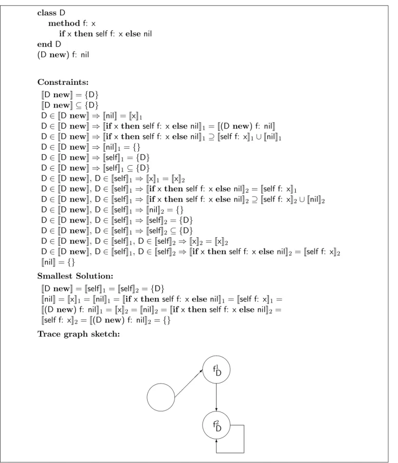
classD

method f: x

ifxthen self f: xelsenil endD (Dnew) f: nil Constraints: [[Dnew]] ={D} [[Dnew]]⊆ {D} D∈[[Dnew]]⇒[[nil]] = [[x]]1

D∈[[Dnew]]⇒[[ifxthen self f: xelsenil]]1= [[(D new) f: nil]]

D∈[[Dnew]]⇒[[ifxthen self f: xelsenil]]1⊇[[self f: x]]1∪[[nil]]1

D∈[[Dnew]]⇒[[nil]]1={}

D∈[[Dnew]]⇒[[self]]1 ={D}

D∈[[Dnew]]⇒[[self]]1 ⊆ {D}

D∈[[Dnew]], D∈[[self]]1 ⇒[[x]]1 = [[x]]2

D∈[[Dnew]], D∈[[self]]1 ⇒[[if xthenself f: xelse nil]]2= [[self f: x]]1

D∈[[Dnew]], D∈[[self]]1 ⇒[[if xthenself f: xelse nil]]2⊇[[self f: x]]2∪[[nil]]2

D∈[[Dnew]], D∈[[self]]1 ⇒[[nil]]2 ={}

D∈[[Dnew]], D∈[[self]]1 ⇒[[self]]2 ={D}

D∈[[Dnew]], D∈[[self]]1 ⇒[[self]]2 ⊆ {D}

D∈[[Dnew]], D∈[[self]]1, D∈[[self]]2⇒[[x]]2 = [[x]]2

D∈[[Dnew]], D∈[[self]]1, D∈[[self]]2⇒[[if xthenself f: x elsenil]]2= [[self f: x]]2 [[nil]] ={}

Smallest Solution:

[[Dnew]] = [[self]]1= [[self]]2={D}

[[nil]] = [[x]]1 = [[nil]]1 = [[if xthenself f: xelse nil]]1= [[self f: x]]1= [[(D new) f: nil]]1 = [[x]]2 = [[nil]]2 = [[if xthenself f: xelse nil]]2= [[self f: x]]2 = [[(D new) f: nil]]2 ={}

Trace graph sketch:

"! # "! # "! # 6 ? f2 D f1 D

(14)

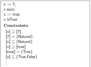
x := 7; x succ; x := true; x isTrue Constraints: [[x]]⊇[[7]] [[7]] ={Natural} [[x]]⊆ {Natural} [[x]]⊇[[true]] [[true]] ={True} [[x]]⊆ {True,False} .. .

Figure 14: A safe program rejected. (ifnil thentrue else7) succ

Constraints:

[[if nil thentrueelse 7]]⊆ {Natural} [[if nil thentrueelse 7]]⊇[[true]]∪[[7]] [[true]] ={True}

[[7]] ={Natural} ..

.

Figure 15: Another safe program rejected. class Studentinherits Comparable

. . . endStudent

class ComparableListinherits List method studentCount

if (self isEmpty) isTrue then 0

else

if(self car) instanceOf Student then((self cdr) studentCount) succ else(self cdr) studentCount

endComparableList

Figure 16: An example program.

Appendix C: Solving Systems of

Conditional Inequalities

This appendix shows how to solve a finite system of conditional inequalities in quadratic time. Definition C.1: A CI-system consists of

• a finite setA ofatoms. • a finite set{αi} of variables.

• a finite set of conditional inequalities of the form

C1, C2, . . . , Ck⇒Q

Each Ci is a condition of the form a ∈ αj,

wherea∈ Ais an atom, andQis aninequality of one of the following forms

A ⊆ αi

αi ⊆ A

αi ⊆ αj

whereA⊆ Ais a set of atoms.

Asolution Lof the system assigns to each variable αi a set L(αi) ⊆ A such that all the conditional

inequalities are satisfied. 2

In our application, A models the set of classes oc-curring in a concrete program.

Lemma C.2: Solutions are closed under intersec-tion. Hence, if a CI-system has solutions, then it has a unique minimal one.

Proof: Consider any conditional inequality of the form C1, C2, . . . , Ck ⇒ Q, and let {Li} be all

so-lutions. We shall show that ∩iLi is a solution. If

a condition a ∈ ∩iLi(αj) is true, then so is all of

a ∈ Li(αj). Hence, if all the conditions of Q are

true in ∩iLi, then they are true in each Li;

fur-thermore, since they are solutions, Q is also true in each Li. Since, in general, Ak ⊆ Bk implies

∩kAk ⊆ ∩kBk, it follows that ∩iLi is a solution.

Hence, if there are any solutions, then ∩iLi is the

unique smallest one. 2

(15)

6 @ @ @ @ @ @ I @ @ @ @ @ @ I error (A,A, . . . ,A) (∅,∅, . . . ,∅)

Figure 17: The lattice of assignments. Aandndistinct variables. Anassignment is an el-ement of (2A)n_{∪ {error}} _{ordered as a lattice, see}

figure 17. If different from error, then it assigns a set of atoms to each variable. IfV is an assignment, then ˜C(V) is a new assignment, defined as follows. If V =error, then ˜C(V) =error. An inequality is enabled if all of its conditions are true underV. If for any enabled inequality of the form αi ⊆ A we

do not have V(αi)⊆A, then ˜C(V) =error;

other-wise, ˜C(V) is the smallest pointwise extension ofV such that

• for every enabled inequality of the form A ⊆ αj we have A⊆C(V˜ )(αj).

• for every enabled inequality of the form αi ⊆

αj we have V(αi)⊆C(V˜ )(αj).

Clearly, ˜C is monotonic in the above lattice. 2

Lemma C.4: An assignment L6=error is a solu-tion of a CI-system C iff L = ˜C(L). If C has no solutions, then error is the smallest fixed-point of

˜ C.

Proof: If L is a solution of C, then clearly ˜C will not equal error and cannot extend L; hence, L is a fixed-point. Conversely, if L is a fixed-point of

˜

C, then all the enabled inequalities must hold. If

there are no solutions, then there can be no fixed-point below error. Since error is by definition a fixed-point, the result follows. 2

This means that to find the smallest solution, or to decide that none exists, we need only compute the least fixed-point of ˜C.

Lemma C.5: For any CI-systemC, the least fixed-point of ˜C is equal to

lim

k→∞ ˜

Ck_(∅,_{∅, . . . ,}_∅)

Proof: This is a standard result about monotonic functions on complete lattices. 2

Lemma C.6: Let n be the number of different conditions in a CI-systemC. Then

lim

k→∞ ˜

Ck_(∅,_{∅, . . . ,}_{∅) = ˜}_Cn+1

(∅,∅, . . . ,∅) Proof: When no more conditions are enabled, then the fixed-point is obtained by a single application. Once a condition is enabled in an assignment, it will remain enabled in all larger assignments. It follows that after n iterations no new conditions can be enabled; hence, the fixed-point is obtained in at most n+ 1 iterations. 2

Lemma C.7: The smallest solution to any CI-system, or the decision that none exists, can be obtained in quadratic time.

Proof: This follows from the previous lemmas. 2

References

[1] Alan H. Borning and Daniel H. H. Ingalls. A type dec-laration and inference system for Smalltalk. InNinth Symposium on Principles of Programming Languages, pages 133–141, 1982.

[2] Luca Cardelli. A semantics of multiple inheri-tance. In Gilles Kahn, David MacQueen, and Gordon Plotkin, editors,Semantics of Data Types, pages 51–68. Springer-Verlag (LNCS 173), 1984.

[3] Luca Cardelli and Peter Wegner. On understanding types, data abstraction, and polymorphism. ACM Computing Surveys, 17(4):471–522, December 1985.

(16)

[4] William Cook and Jens Palsberg. A denotational se-mantics of inheritance and its correctness. Information and Computation, 114(2):329–350, 1994. Also in Proc. OOPSLA’89, ACM SIGPLAN Fourth Annual Confer-ence on Object-Oriented Programming Systems, Lan-guages and Applications, pages 433–443, New Orleans, Louisiana, October 1989.

[5] William R. Cook. A Denotational Semantics of Inher-itance. PhD thesis, Brown University, 1989.

[6] Ole-Johan Dahl, Bjørn Myhrhaug, and Kristen Ny-gaard. Simula 67 common base language. Technical report, Norwegian Computing Center, Oslo, Norway, 1968.

[7] Scott Danforth and Chris Tomlinson. Type theories and object-oriented programming. ACM Computing Sur-veys, 20(1):29–72, March 1988.

[8] Adele Goldberg and David Robson.Smalltalk-80—The Language and its Implementation. Addison-Wesley, 1983.

[9] Justin O. Graver and Ralph E. Johnson. A type system for Smalltalk. InSeventeenth Symposium on Principles of Programming Languages, pages 136–150, 1990. [10] Justin Owen Graver.Type-Checking and Type-Inference

for Object-Oriented Programming Languages. PhD the-sis, Department of Computer Science, University of Illi-nois at Urbana-Champaign, August 1989. UIUCD-R-89-1539.

[11] Andreas V. Hense. Polymorphic type inference for a simple object oriented programming language with state. Technical Report No. A 20/90, Fachbericht 14, Universit¨at des Saarlandes, December 1990.

[12] Ralph E. Johnson. Type-checking Smalltalk. InProc. OOPSLA’86, Object-Oriented Programming Systems, Languages and Applications, pages 315–321. Sigplan Notices, 21(11), November 1986.

[13] Samuel Kamin. Inheritance in Smalltalk–80: A denota-tional definition. InFifteenth Symposium on Principles of Programming Languages, pages 80–87, 1988. [14] Marc A. Kaplan and Jeffrey D. Ullman. A general

scheme for the automatic inference of variable types. InFifth Symposium on Principles of Programming Lan-guages, pages 60–75, 1978.

[15] Bent B. Kristensen, Ole Lehrmann Madsen, Birger Møller-Pedersen, and Kristen Nygaard. The BETA pro-gramming language. In Bruce Shriver and Peter Weg-ner, editors, Research Directions in Object-Oriented Programming, pages 7–48. MIT Press, 1987.

[16] Harry G. Mairson. Decidability of ML typing is com-plete for deterministic exponential time. InSeventeenth Symposium on Principles of Programming Languages, pages 382–401, 1990.

[17] Bertrand Meyer. Object-Oriented Software Construc-tion. Prentice-Hall, Englewood Cliffs, NJ, 1988.

[18] Robin Milner. A theory of type polymorphism in pro-gramming. Journal of Computer and System Sciences, 17:348–375, 1978.

[19] Prateek Mishra and Uday S. Reddy. Declaration-free type checking. InTwelfth Symposium on Principles of Programming Languages, pages 7–21, 1985.

[20] Jens Palsberg and Michael I. Schwartzbach. Type sub-stitution for object-oriented programming. In Proc. OOPSLA/ECOOP’90, ACM SIGPLAN Fifth Annual Conference on Object-Oriented Programming Systems, Languages and Applications; European Conference on Object-Oriented Programming, pages 151–160, Ottawa, Canada, October 1990.

[21] Jens Palsberg and Michael I. Schwartzbach. What is type-safe code reuse? InProc. ECOOP’91, Fifth Eu-ropean Conference on Object-Oriented Programming, pages 325–341. Springer-Verlag (LNCS 512), Geneva, Switzerland, July 1991.

[22] Jens Palsberg and Michael I. Schwartzbach. Static typ-ing for object-oriented programmtyp-ing. Science of Com-puter Programming, 23(1):19–53, 1994.

[23] Uday S. Reddy. Objects as closures: Abstract semantics of object-oriented languages. InProc. ACM Conference on Lisp and Functional Programming, pages 289–297, 1988.

[24] Didier R´emy. Typechecking records and variants in a natural extension of ML. In Sixteenth Symposium on Principles of Programming Languages, pages 77–88, 1989.

[25] Michael I. Schwartzbach. Type inference with inequal-ities. InProc. TAPSOFT’91, pages 441–455. Springer-Verlag (LNCS 493), 1991.

[26] Bjarne Stroustrup. The C++ _{Programming Language}_.

Addison-Wesley, 1986.

[27] Norihisa Suzuki. Inferring types in Smalltalk. InEighth Symposium on Principles of Programming Languages, pages 187–199, 1981.

[28] Mitchell Wand. A simple algorithm and proof for type inference.Fundamentae Informaticae, X:115–122, 1987. [29] Mitchell Wand. Type inference for record concatenation and multiple inheritance. InLICS’89, Fourth Annual Symposium on Logic in Computer Science, pages 92–97, 1989.