Measures of explained variance and pooling in multilevel models

Measures of explained variance and pooling in multilevel models

Andrew Gelman, Columbia University

Iain Pardoe, University of Oregon

Contact: Iain Pardoe, Charles H. Lundquist College of Business,

University of Oregon, Eugene, OR 97403–1208 ([email protected])

infer-ence; Hierarchical model; Multilevel regression; Par-tial pooling; Shrinkage.

Abstract:

Explained variance (R-squared) has been general-ized in various ways to multilevel models for hi-erarchical data structures in which individuals are grouped into units, and there are variables measured on individuals and each grouping unit. The mod-els are based on regression relationships at different levels, with the first level corresponding to the in-dividual data, and subsequent levels corresponding to between-group regressions of individual predic-tor effects on grouping unit variables. We present an approach to defining R-squared at each level of the multilevel model, rather than attempting to cre-ate a single summary measure of fit, by compar-ing variances within the model. In simple regres-sion, our measure generalizes the classical adjusted R-squared. We also discuss a related variance com-parison to summarize the degree to which estimates at each level of the model are pooled together based on the level-specific regression relationship, rather than estimated separately. This pooling factor is re-lated to the concept of shrinkage in simple hierarchi-cal models. We illustrate the methods on a dataset of radon in houses within counties using a series of multilevel models.

1.

Introduction

1.1 Explained variation in linear models Consider a linear regression written asyi= (Xβ)i+

²i, i = 1, . . . , n. The fit of the regression can be

summarized by the proportion of variance explained:

R2_{= 1−} V n i=1²i Vn i=1yi , (1)

where V represents the finite-sample variance op-erator, Vn i=1xi = 1 n−1 P_n i=1(xi−x¯)2. In a multilevel

model (that is, a hierarchical model with group-level error terms or with regression coefficientsβthat vary

by group), the predictors “explain” the data at dif-ferent levels, and R2 _{can be generalized in a}

vari-ety of ways (for textbook summaries, see Kreft and De Leeuw, 1998; Snijders and Bosker, 1999; Rauden-bush and Bryk, 2002; Hox, 2002). Xu (2003) reviews some of these approaches, their connections to in-formation theory, and similar measures for general-ized linear models and proportional hazards models. Hodges (1998) discusses connections between hier-archical linear models and classical regression.

The definitions of “explained variance” that we have seen are based on comparisons with a null model, so that R2 _{is equal to 1 −}

residual variance under the larger model

residual variance under the null model , with var-ious choices of the null model corresponding to pre-dictions at different levels.

In this paper we shall propose a slightly different approach, computing (1) at each level of the model and thus coming up with several R2 _{values for any}

particular multilevel model. This approach has the virtue of summarizing the fit at each level and re-quiring no additional null models to be fit. In defin-ing this summary, our goal is not to dismiss other definitions of R2 _{but rather to add another tool to}

the understanding of multilevel models. 1.2 Pooling in hierarchical models

Multilevel models are often understood in terms of “partial pooling,” compromising between un-pooled and completely un-pooled estimates. For ex-ample, the basic hierarchical model involves data

yj ∼ N(αj, σy2), with population distribution αj ∼

N(µα, σα2) and known hyperparameters µα, σy, σα.

For each group j, the multilevel estimate of αj is

ˆ αmultilevel j =ωµα+ (1−ω)yj, (2) where ω= 1− σ 2 α σ2 α+σy2 (3) is a “pooling factor” that represents the degree to which the estimates are pooled together (that is, based on µα) rather than estimated separately

(based on the raw data yj). The extreme

possi-bilities, ω = 0 and 1, correspond to no pooling (ˆαj =yj) and complete pooling (ˆαj =µα),

is var(αj) = (1−ω)σ2y. The statistical literature

sometimes labels 1−ω as the “shrinkage” factor, a notation we find confusing since a shrinkage factor of zero corresponds to complete shrinkage towards the population mean. To avoid ambiguity, we use the term “pooling factor” in this paper. The form of expression (3) matches the form of the definition (1) ofR2_{, a parallelism we shall continue throughout.}

The concept of pooling aids understanding of mul-tilevel models in two distinct ways: comparing the estimates of different parameters in a group, and summarizing the pooling of the model as a whole. When comparing, it is usual to consider several pa-rametersαj with a common population (prior)

dis-tribution but different data variances; thus, yj ∼

N(αj, σy j2 ). Then ωj can be defined as in (3), with

σy j in place of σy. Parameters with more precise

data are pooled less towards the population mean, and this can be displayed graphically by a parallel coordinate plot showing the raw estimatesyjpooled

toward the posterior means ˆαmultilevel

j , or a

scatter-plot of ˆαmultilevel

j vs. yj. Pooling of the model as a

whole makes use of the fact that the multilevel esti-mates of the individual parametersαj, if treated as

point estimates, understate the between-group vari-ance (Louis, 1984). See Efron and Morris (1975) and Morris (1983) for discussions of pooling and shrink-age in hierarchical or “empirical Bayes” inference.

In this paper we present a summary measure, λ, for the average amount of pooling at each level of a multilevel model. We shall introduce an example to motivate the need for such summaries, and then discuss the method and illustrate its application. 1.3 Example: home radon levels

In general, each level of a multilevel model can have regression predictors and variance components. In this paper, we propose summary measures of ex-plained variation and pooling that are defined and computed at each model level. We demonstrate with an example adapted from our own research— a varying-intercept, varying-slope model for radon gas levels in houses clustered within counties. The model has predictors for both houses and counties, and we introduce it here in order to show the chal-lenges in definingR2 _{andλin a multilevel context.}

Radon is a carcinogen—a naturally occurring radioactive gas whose decay products are also radioactive—known to cause lung cancer in high concentration, and estimated to cause several thou-sand lung cancer deaths per year in the United States. The distribution of radon levels in U.S. houses varies greatly, with some houses having dan-gerously high concentrations. In order to identify

the areas with high radon exposures, the Environ-mental Protection Agency coordinated radon mea-surements in each of the 50 states.

We illustrate here with an analysis of measured radon in 919 houses in the 85 counties of Min-nesota. In performing the analysis, we use a house predictor—whether the measurement was taken in a basement (radon comes from underground and can enter more easily when a house is built into the ground). We also have an important county predictor—a county-level measurement of soil ura-nium content. We fit the following model,

yij ∼ N(αj+βj·basementij, σy2),

fori= 1, . . . , nj, j = 1, . . . , J

αj ∼ N(γ0+γ1uj, σα2), forj= 1, . . . , J

βj ∼ N(δ0+δ1uj, σβ2), forj = 1, . . . , J, (4)

whereyijis the logarithm of the radon measurement

in house i in county j, basementij is the indicator

for whether the measurement was in a basement, and

uj is the logarithm of the uranium measurement in

countyj. The errors in the first line of (4) represent within-county variation, which in this case includes measurement error, natural variation in radon lev-els within a house over time, and variation among houses (beyond that explained by the basement in-dicator). The errors in the second and third lines represent variations in radon levels and basement effects between counties, beyond that explained by the county-level uranium predictor. The between-county errors, αj and βj, are modeled as

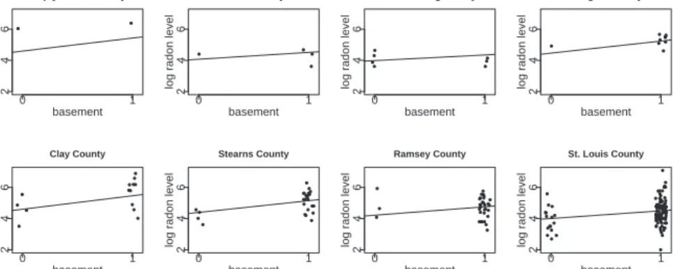
indepen-dent (see Section 5 for discussion of this point). The hierarchical model fits a regression to the in-dividual measurements while accounting for system-atic unexplained variation among the 85 counties. Figure 1 shows the data and fitted regression lines within counties, and Figure 2 shows the estimated county parameters and county-level regression lines. This example illustrates some of the challenges of measuring explained variance and pooling. The model has three levels, with a different variance com-ponent at each level. Here, “levels” correspond to the separate variance components rather than to the more usual measurement scales (of which there are two in this case, house and county). Uncertainty in the αand β parameters affects the computation of explained variance for the data-level model—the simple measure of R2 _{from least-squares regression}

will not be appropriate—and also for the county-level models, since these are regressions with out-comes that are estimated, not directly observed.

In summarizing the pooling of a batch of param-eters in a multilevel model, expression (3) cannot in

Laq Qui Parle County

basement

log radon level

0 1 2 4 6 Aitkin County basement

log radon level

0 1 2 4 6 Koochiching County basement

log radon level

0 1 2 4 6 Douglas County basement

log radon level

0 1 2 4 6 Clay County basement

log radon level

0 1 2 4 6 Stearns County basement

log radon level

0 1 2 4 6 Ramsey County basement

log radon level

0 1 2 4 6 St. Louis County basement

log radon level

0 1

2

4

6

Figure 1: Jittered data and estimated regression lines from the multilevel model, y =αj+βj·basement,

for radon data, displayed for 8 of the 85 counties j in Minnesota. Both the intercept and the slope vary by county. Because of the pooling of the multilevel model, the fitted lines do not go through the center of the data, a pattern especially noticeable for counties with few observations.

3.8 4.0 4.2 4.4 4.6 4.8

county−level uranium measure

regression intercept −0.5 0.0 0.5 0.2 0.4 0.6 0.8 1.0

county−level uranium measure

regression slope

−0.5 0.0 0.5

Figure 2: (a) Estimates ±standard errors for the county intercepts αj, plotted vs. county-level uranium

measurement uj, along with the estimated multilevel regression line, α = γ0+γ1u. (b) Estimates ± standard errors for the county slopesβj, plotted vs.uj, along with the estimated multilevel regression line, β=δ0+δ1u. For each graph, the county coefficients roughly follow the line but not exactly; the discrepancies of the coefficients from the line are summarized by the hierarchical standard deviation parametersσα, σβ. general be used directly—the difficulty is that it

re-quires knowledge of the unpooled estimates, yj, in

(2). In the varying-intercept, varying-slope radon model, the unpooled estimates are not necessarily available, for example in a county where all the mea-sured houses have the same basement status.

These difficulties inspire us to define measures of explained variance and pooling that do not depend on fitting alternative models but rather summarize variances within a single fitted multilevel model.

2.

Summaries based on variance

com-parisons within a single model

fac-tors for each level of a multilevel model and then in Section 2.5 describe how to compute these

sum-maries using Bayesian posterior simulation draws. 2.1 Notation

We begin by defining a standard notation for a mul-tilevel model with M levels. (For example, M = 3 in the radon model of Section 1.3.) At each levelm, we write the model as,

θ_k(m)=µ(_km)+²_k(m), fork= 1, . . . , K(m)_{, (5)}

where the µ(_km)’s are the linear predictors at that level of the model and the errors ²(_km) come from a distribution with mean zero and standard deviation

σ(m)_{. At the lowest (data) level of the model, the} θ(_km)’s correspond to the individual data points (the

yij’s in the radon model). At higher levels of the

model, the θ(_km)’s represent batches of effects or re-gression coefficients (county interceptsαjand slopes

βj in the radon model). Because we work with each

level of the model separately, we shall suppress the superscripts (m) for the rest of the paper.

The striking similarity of expressions (1) and (3), which define R2 _{and λ, respectively, suggests that}

the two concepts can be understood in a common framework. We consider each to represent the frac-tion of variance explained, first by the linear predic-torµand then by the hierarchical model for². 2.2 Variance explained at each level

For each level (5) of the model, we first consider the variance explained by the linear predictors µk.

Generalizing from the classical expression (1), we define R2= 1− E µ VK k=1²k ¶ E µ VK k=1θk ¶. (6) In a Bayesian simulation context, the expectations in the numerator and denominator of (6) can be eval-uated by averaging over posterior simulation draws, as we discuss in Section 2.5.

R2 _{will be close to 0 when the average residual}

error variance is approximately equal to the average variance of the θk’s. R2 will be close to 1 when

the residual errors²k are each close to zero for each

posterior sample. Thus R2 _{is larger when the µ}

k’s

more closely approximate theθk’s.

In classical least-squares regression, (6) reduces to the usual definition ofR2_{: the numerator of the ratio}

becomes the residual variance, and the denominator is simply the variance of the data. Averaging over uncertainty in the regression coefficients leads to a lower value for R2_{, as with the classical “adjusted} R2_{” measure (Wherry, 1931). We discuss this}

con-nection further in Section 3.1. It is possible for our measure (6) to be negative, much like adjustedR2_,

if a model predicts so poorly that, on average, the residual error variance is larger than the variance of the data.

2.3 Pooling factor at each level

The next step is to summarize the extent to which the variance of the residuals ²k is reduced by the

pooling of the hierarchical model. We define the pooling factor as λ= 1− V K k=1E(²k) E µ VK k=1²k ¶. (7) The denominator in this expression is the numerator in expression (6)—the average variance in the ²k’s,

that is, the unexplained component of the variance of theθk’s. The numerator in the ratio term of (7) is

the variance among the point estimates (the shrink-age estimators) of the ²k’s. If this variance is high

(close to the average variance in the ²k’s), then λ

will be close to 0 and there is little pooling. If this variance is low, then the estimated ²k’s are pooled

closely together, and the pooling factor λ will be close to 1.

In Section 3.2, we discuss connections between the pooling factor (7) and the pooling factor ω defined in (3) for the basic hierarchical model.

2.4 Properties of the summary measures Since R2 _{and λare based on finite-population}

vari-ances, they are well-defined for each level of a mul-tilevel model, and automatically work even in the presence of predictors at that level. An alternative approach based on hyperparameters could run into difficulties in such situations since the hyperparame-ters may not correspond exactly to the variance com-parisons we are interested in.

As a model improves (by adding better predictors and thus improving the µk’s), we would generally

expect both R2 _{and λ to increase for all levels of}

the model. Increasing R2 _{corresponds to more of}

the variation being explained at that level of the regression model, and a high value ofλimplies that the model is pooling the ²k’s strongly towards the

population mean for that level.

Adding a predictor at one level doesnot necessar-ily increase R2 _{and λat other levels of the model,}

however. In fact, it is possible for an individual-level predictor to improve prediction at the data level but decrease R2 _{at the group level (see Kreft and De}

Leeuw, 1998; Gelman and Price, 1998; Hox, 2002, for discussion and examples of this phenomenon). For the purpose of this paper, we merely note that a model can have different explanatory power at dif-ferent levels.

2.5 Posterior simulation computations Multilevel models are increasingly evaluated in a Bayesian framework and computed using posterior simulation, in which inferences for the vector of pa-rameters are summarized by a matrix of simulations (see, e.g., Gilks et al., 1996; Carlin and Louis, 2000; Gelman et al., 2003).

We can then evaluate R2 _{and λ at each level m}

of the model using the posterior simulations (not simply the parameter estimates or posterior means), as follows:

Evaluate R2 _{from (6):}

1. From each simulation draw of the model param-eters:

(a) Compute the vector ofθk’s, predicted

val-ues µk and the vector of residuals, ²k =

θk−µk.

(b) Compute the sample variances, VK

k=1θk and

VK

k=1²k.

2. Average over the simulation draws to estimate E µ V K k=1θk ¶ and E µ V K k=1²k ¶

, and then use these to calculateR2_.

Evaluate λ from (7) using these same simulation draws in a different way:

1. For each k, estimate the posterior mean E(²k)

of each of the errors ²k as defined in step 1(a)

above.

2. Compute the variance of the K values of E(²k), V

K

k=1E(²k), and then use this, along with

E( VK

k=1²k) from step 2 above to calculateλ.

3.

Connections to classical definitions

The classical normal linear regression model can be written asyi = (Xβ)i+²i, i= 1, . . . , n, with linear

predictors (Xβ)i and errors²i that are normal with

zero mean and constant varianceσ2_.

If we plug in the least-squares estimate, ˆβ = (XT_X)−1_XT_{y, then the proportion of variance}

ex-plained (6) simply reduces to the classical definition,

R2_{= 1−}E ³ Vn i=1²i ´ E ³ Vn i=1yi ´ = 1−yT(I−H)y yT_I cy ,

where I is the n × n identity matrix, H =

X(XT_X)−1_XT_{, and I}

c is the n×n matrix with

1−1/nalong the diagonal and 1/noff the diagonal. In a Bayesian context, to fully evaluate our expres-sion (6) forR2_{, one would also average over posterior}

uncertainty inβ andσ. Under the standard nonin-formative prior density that is uniform on (β,logσ), the proportion of variance explained (6) becomes,

R2= 1− µ n−3 n−p−2 ¶ yT_(I−H)y yT_I cy ,

wherepis the number of columns ofX.

This is remarkably similar to the classical adjusted

R2_{. In fact, if we plug in the classical estimate,}

ˆ

σ2_=yT_{(I−H)y/(n−p), rather than averaging over}

the marginal posterior distribution forσ2_{, then (6)}

becomes R2_{= 1−} µ n−1 n−p ¶ yT_(I−H)y yT_Icy ,

which is exactly classical adjusted R2_{. Since}

n−3

n−p−2>nn−−1p for p >1, our “Bayesian adjustedR2”

leads to a lower measure of explained variance than the classical adjusted R2_{. This makes sense, since}

the classical adjusted R2 _{could be considered too}

high since it does not account for uncertainty inσ. The pooling factor defined in (7) also has a simple form. Evaluating the expectations over the poste-rior distribution yields λ= 1−(n−p−2)/(n−3). If we plug in the classical estimate, ˆσ2 _{= y}T_(I−

H)y/(n−p), rather than averaging over the marginal posterior distribution for σ2_{, then (7) becomesλ=}

1−(n−p)/(n−1). We can see that in the usual setting where the number of regression predictors,p, is small compared to the sample size,n, this pooling factorλfor the regression errors will be close to zero. This makes sense because, in this case, the classical residuals (y−Xβˆ)iare nearly independent, and they

closely approximate the errors²i= (y−Xβ)i. Thus,

very little shrinkage is needed to estimate these un-observed²i’s.

3.2 One-way hierarchical model

The one-way hierarchical model has the form,yij∼

N(αj, σ2y), i= 1, . . . , nj, j= 1, . . . , J, with

popula-tion distribupopula-tion αj ∼N(µα, σα2), and we can

deter-mine the appropriate variance comparisons at each of the two levels of the model. For simplicity, we assume that the within-group sample sizesnjare all

equal to a common value n, so that the total sam-ple size isN =nJ. The basic hierarchical model of Section 1.2 corresponds to the special case ofn= 1. We use the usual noninformative prior density that is uniform on (µα,logσy, σα). It is not possible

to derive closed-form expressions for (6) and (7) av-eraging over the full posterior distribution. Instead, we present plug-in expressions using the method-of-moments estimators, ˆ σ2 α+ ˆσy2/n = yT_I¯ cy N , ˆ σ2 y = yT_(I c−I¯c)y N , (8)

wherey= (y11, . . . , yn1, . . . , y1J, . . . , ynJ)T is theN

-vector of responses, ¯Ic is the N×N block-diagonal

matrix with n × n matrices containing elements 1/n−1/N along the diagonal and n×n matrices containing elements −1/N off the diagonal, and Ic

is theN×N matrix with 1−1/N along the diagonal and −1/N off the diagonal. Thus, the first esti-mator in (8) is the sample variance of the J group means (rescaled by (J−1)/J), while the second esti-mator is the pooled within-group variance (rescaled by (n−1)/n).

Conditional onσy andσα, the proportion of

vari-ance explained, (6), at the data level is

R2_{= 1−}yT(Ic−I¯c)y+ω2yTI¯cy+J(1−ω)σy2

yT_I cy

.

Plugging in the estimators (8) leads to

R2 = 1− µ n+ 1 n ¶ yT_(I c−I¯c)y yT_I cy = 1− σˆ 2 y/n ˆ σ2 α/(n+ 1) + ˆσy2/n .

Subject to finite-sample size adjustments, this is ap-proximately equal to the usual value forR2 _{in this}

model, 1−σ2

y/(σ2α+σy2).

Conditional onσy andσα, the pooling factor, (7),

at the data level is

λ= 1− y T_(I c−I¯c)y+ω2yTI¯cy yT_(Ic−I¯_c)y+ω2_yT_I¯_{cy+J(1−ω)σ}2 y .

Plugging in the estimators (8) leads to

λ = 1−n 2_yT_I¯ cy+yT(Ic−I¯c)y n(n+ 1)yT_I¯ cy = 1− n n+1σˆ2α+ ˆσ2y/n ˆ σ2 α+ ˆσ2y/n .

If the within-group sample sizes n are reason-ably large, this data-level pooling factor λ is close to zero, which makes sense because the data-level residuals are good approximations to the data-level errors (similar to the case of classical regression as discussed in Section 3.1).

At the group level, the one-way hierarchical model has no predictors, and soR2_{= 0.}

Conditional onσy andσα, the pooling factor, (7),

at the group level is

λ= 1− (1−ω)yTI¯cy

(1−ω)yT_I¯_{cy+J σ}2

y

.

Plugging in the estimators in (8) leads to

λ = 1−n y T_I¯ cy−yT(Ic−I¯c)y n yT_I¯ cy = 1− ˆσ 2 α ˆ σ2 α+ ˆσy2/n .

This expression reduces to (3) by settingnequal to 1 for the basic hierarchical model of Section 1.2.

4.

Applied example

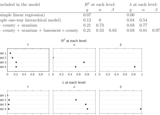
We fit four models to the example from Section 1.3 of home radon levels. Figure 3 shows the proportion of explained variance and pooling factor for each level of each model, as computed directly from posterior simulation draws as described in Section 2.5. We discuss the results for each model in turn:

Model 1. A simple linear regression of log radon level on basement indicators, illustrating the theo-retical calculations of Section 3.1:

R2 _{is very low, suggesting a poorly fitting model,}

and λ is essentially zero, indicating that the errors are estimated almost independently (which gener-ally holds for a data-level regression model in which there are many more data points than predictors). By comparison, the classical R2 _{for this}

regres-sion, plugging in the least-squares estimate for β, is 1−yT_(I−H)y/yT_I

cy = 0.07. The theoretical

value forλfor this model, is 1−(n−3)/(n−p−2) = 0.07. These results are all essentially the same be-cause there is very little uncertainty inβandσwhen fitting this simple model, hence little is changed by moving to fully-Bayesian inference.

Model 2. A simple one-way hierarchical model of houses within counties, extending the theoretical calculations of Section 3.2 to account for unequal sample sizes and variance parameter uncertainty:

At the data level, R2 _{shows some improvement}

over the simple linear regression model but is still quite low. The pooling factor λ remains close to zero. If there were equal sample sizes within each county, the theoretical value for R2 _{for this data}

level model, based on plugging in the estimators (8), comes to 0.13. Using the posterior simulations ac-counts for unequal sample sizes and uncertainty in the variance parameters. Similarly, the approximate value forλfor this data level model, plugging in the estimators (8), comes to 0.05.

At the county level,R2_{= 0 since this model has no}

county-level predictors. The pooling factorλ= 0.54 indicates that county mean estimates are weighted about equally between county sample means and the overall population mean. If there were equal sample sizes within each county, the calculated value for λ

for this county level model, plugging in the estima-tors (8), comes to 0.37. In this case, accounting for unequal sample sizes and variance parameter uncer-tainty leads to a very different result.

Model 3. A varying-intercept hierarchical model, with basement as an individual-level predictor and log uranium as a county-level predictor:

At the data level, R2 _{improves further over the}

one-way hierarchical model but still remains quite low. The pooling factor λremains close to zero.

For the intercept model,R2_{= 0.73 indicates that}

when we restrict basement effects to be the same in all counties, uranium level explains about three-quarters of the variation among counties. The pool-ing factor implies that county mean estimates are pooled on average about 80% toward the regression line predicting county means from uranium levels.

Predictors included in the model R2 _{at each level: λat each level:}

y α β y α β

Basement (simple linear regression) 0.07 0.00

County (simple one-way hierarchical model) 0.12 0 0.04 0.54

Basement + county + uranium 0.21 0.73 0.03 0.77

Basement + county + uranium + basement×county 0.21 0.53 0.83 0.03 0.81 0.97

y Model 4 Model 3 Model 2 Model 1 0 0.2 0.4 0.6 0.8 1 α 0 0.2 0.4 0.6 0.8 1 β 0 0.2 0.4 0.6 0.8 1 R2 at each level: y Model 4 Model 3 Model 2 Model 1 0 0.2 0.4 0.6 0.8 1 α 0 0.2 0.4 0.6 0.8 1 β 0 0.2 0.4 0.6 0.8 1 λ at each level:

Figure 3: Proportion of variance explained and pooling factor at the level of datay, county-level intercepts

α, and county-level slopesβ, for each of four models fit to the Minnesota radon data. Blank entries indicate variance components that are not present in the given model. Results shown in tabular and graphical forms.

Model 4. The full intercept, varying-slope model (4), in which the basement effect β is allowed to vary by county:

At the data level,R2 _{is still quite low, indicating}

that much of the variation in the data remains un-explained by the model (as can be seen in Figure 1), andλis still close to zero.

For the intercept modelR2_{close to 50% indicates}

that uranium level explains about half the varia-tion among counties, and λ close to 80% implies that there is little additional information remaining about each county’s intercept. The estimates are pooled on average about 80% toward the regression line (as is apparent in Figure 2a). R2 _{at the}

inter-cept level has decreased from the previous model in which basement effects are restricted to be the same in all counties; allowing the basement effects to vary by county means that there is less variation remain-ing between counties for uranium level to explain.

For the slope model, R2 _{is over 80%, implying}

that the uranium level explains much of the system-atic variation in the basement effects across counties. The pooling factorλis almost all the way to 1, which tells us that the slopes are almost entirely estimated from the county-level model, with almost no addi-tional information about the individual counties (as

can be seen in Figure 2b).

The fact that much of the information in R2 _and λis captured in Figures 1 and 2 should not be taken as a flaw of these measures. Just as the correlation is a useful numerical summary of information available in a scatterplot, the explained variance and pooling measures quickly summarize the explanatory power and actions of a multilevel model, without being a substitute for more informative graphical displays.

5.

Discussion

We suggest computing our measures for the propor-tion of variance explained at each level of a multi-level model, (6), and the pooling factor at each multi-level, (7). These can be easily calculated using posterior simulations as detailed in Section 2.5. The mea-sures of R2 _{andλconveniently summarize the fit at}

each level of the model and the degree to which esti-mates are pooled towards their population models. Together, they clarify the role of predictors at differ-ent levels of a multilevel model. They can be derived from a common framework of comparing variances at each level of the model, which also means that they do not require the fitting of additional null models.

usual definitions of adjustedR2 _{in simple linear}

re-gression and shrinkage in balanced one-way hierar-chical models. From this perspective, they unify the data-level concept ofR2_{and the group-level concept}

of pooling or shrinkage, and also generalize these concepts to account for uncertainty in the variance components. Further, as illustrated for the home radon application in Section 4, they provide a useful tool for understanding the behavior of more complex multilevel models.

We define R2 _{and λat each level of a multilevel}

model, where the error terms at each level are mod-eled as independent. However, models such as the full varying-intercept, varying-slope model used in the home radon application can be generalized to allow for correlated intercepts and slopes. The as-sumption of uncorrelated intercepts and slopes is of-ten reasonable when there are useful predictors avail-able for each grouping unit (as is the case for the home radon application). Nevertheless, it would be useful to extendR2_{andλfor use in situations where}

such an assumption was not reasonable.

We have presented our R2 _{and λ measures in a}

Bayesian framework. However, they could also be evaluated in a non-Bayesian framework using sim-ulations from distributions representing estimates and measures of uncertainty for the predicted values

µk and the residuals ²k. For example, these might

be represented by multivariate normal distributions with a point estimate for the mean and estimated covariance matrix for the variance, or alternatively by bootstrap simulations.

We have derived connections to classical defini-tions of explained variance and shrinkage for models with normal error distributions, and illustrated our methods using a multilevel model with normal errors at each level. However, (6) and (7) do not depend on any normality assumptions, and, in principle, these measures are appropriate variance summaries for models with nonnormal error distributions (see also Goldstein et al., 2002; Browne et al., 2003). It may be possible to develop analogous measures us-ing deviances for generalized linear models.

References

Browne, W. J., S. V. Subramanian, K. Jones, and H. Goldstein (2003). Variance partitioning in mul-tilevel logistic models that exhibit over-dispersion. Technical report, School of Mathematical Sci-ences, University of Nottingham.

Carlin, B. P. and T. A. Louis (2000). Bayes and Empirical Bayes Methods for Data Analysis (2nd ed.). Boca Raton, FL: Chapman & Hall/CRC.

Efron, B. and C. Morris (1975). Data analysis using stein’s estimator and its generalizations. Journal of the American Statistical Association 70, 311– 319.

Gelman, A., J. B. Carlin, H. S. Stern, and D. B. Rubin (2003). Bayesian Data Analysis (2nd ed.). Boca Raton, FL: Chapman & Hall/CRC.

Gelman, A. and P. N. Price (1998). Discussion of “Some algebra and geometry for hierarchical models, applied to diagnostics,” by J. S. Hodges.

Journal of the Royal Statistical Society, Series B (Methodological).

Gilks, W. R., S. Richardson, and D. J. Spiegelhal-ter (Eds.) (1996). Markov Chain Monte Carlo in Practice. Boca Raton, FL: Chapman & Hall/CRC.

Goldstein, H., W. J. Browne, and J. Rasbash (2002). Partitioning variation in multilevel models. Un-derstanding Statistics 1, 223–232.

Hodges, J. S. (1998). Some algebra and geometry for hierarchical models, applied to diagnostics. JRSS-B 60, 497–536.

Hox, J. (2002). Multilevel Analysis: Techniques and Applications. Mahwah, NJ: Lawrence Erlbaum Associates.

Kreft, I. and J. De Leeuw (1998). Introducing Mul-tilevel Modeling. London: Sage.

Louis, T. A. (1984). Estimating a population of pa-rameter values using bayes and empirical bayes methods. Journal of the American Statistical As-sociation 78, 393–398.

Morris, C. (1983). Parametric empirical bayes in-ference: theory and applications (with discus-sion). Journal of the American Statistical Associ-ation 78, 47–65.

Raudenbush, S. W. and A. S. Bryk (2002). Hierar-chical Linear Models (2nd ed.). Thousand Oaks, CA: Sage.

Snijders, T. A. B. and R. J. Bosker (1999).Multilevel Analysis. London: Sage.

Wherry, R. J. (1931). A new formula for predicting the shrinkage of the coefficient of multiple corre-lation. Annals of Mathematical Statistics 2, 440– 457.

Xu, R. (2003). Measuring explained variation in linear mixed effects models. Statistics in Medicine 22, 3527–3541.