The learnability of voting rules

Contents lists available atScienceDirect

Artificial Intelligence

www.elsevier.com/locate/artint

The learnability of voting rules

✩

Ariel D. Procaccia

a

,

∗

,

1

, Aviv Zohar

b

,

a

, Yoni Peleg

b

, Jeffrey S. Rosenschein

b

a_{Microsoft Israel R&D Center, 13 Shenkar Street, Herzeliya 46725, Israel}

b_{School of Computer Science and Engineering, The Hebrew University of Jerusalem, Jerusalem 91904, Israel}

a r t i c l e i n f o a b s t r a c t

Article history: Received 16 May 2008

Received in revised form 25 March 2009 Accepted 27 March 2009

Available online 9 April 2009 Keywords:

Computational social choice Computational learning theory Multiagent systems

Scoring rules and voting trees are two broad and concisely-representable classes of voting rules; scoring rules award points to alternatives according to their position in the preferences of the voters, while voting trees are iterative procedures that select an alternative based on pairwise comparisons. In this paper, we investigate the PAC-learnability of these classes of rules. We demonstrate that the class of scoring rules, as functions from preferences into alternatives, is efficiently learnable in the PAC model. With respect to voting trees, while in general a learning algorithm would require an exponential number of samples, we show that if the number of leaves is polynomial in the size of the set of alternatives, then a polynomial training set suffices. We apply these results in an emerging theory: automated design of voting rules by learning.

©2009 Elsevier B.V. All rights reserved.

1. Introduction

Voting is a well-studied method of preference aggregation, in terms of its theoretical properties, as well as its computa-tional aspects [6,21]; various practical, implemented applications that use voting exist [9,12,13].

In an election,n voters express their preferences over a set ofm alternatives. To be precise, each voter is assumed to

reveal linear preferences—a ranking of the alternatives. The outcome of the election is determined according to avoting rule.

In this paper we will consider two families of voting rules: scoring rules and voting trees.

Scoring rules. The predominant—ubiquitous, even—voting rule in real-life elections is thePluralityrule. Under Plurality, each voter awards one point to the alternative it ranks first, i.e., its most preferred alternative. The alternative that accumulated

the most points, summed over all voters, wins the election. Another example of a voting rule is theVetorule: each voter

“vetoes” a single alternative; the alternative that was vetoed by the fewest voters wins the election. Yet a third example

is theBordarule: every voter awardsm

−

1 points to its top-ranked alternative, m

−

2 points to its second choice, and so

forth—the least preferred alternative is not awarded any points. Once again, the alternative with the most points is elected.

The above-mentioned three voting rules all belong to an important family of voting rules known asscoring rules. A scoring

rule can be expressed by a vector of parameters

α

=

α

1

,

α

2

, . . . ,

α

m

, where each

α

l is a real number and

α

1

α

2

· · ·

α

m. Each voter awards

α

1 points to its most-preferred alternative,

α

2 to its second-most-preferred alternative, etc.

Predictably, the alternative with the most points wins. Under this unified framework, we can express our three rules as:

✩ _{This paper subsumes two earlier conference papers [A.D. Procaccia, A. Zohar, Y. Peleg, J.S. Rosenschein, Learning voting trees, in: Proceedings of the 22nd}

AAAI Conference on AI (AAAI), 2007, pp. 110–115; A.D. Procaccia, A. Zohar, J.S. Rosenschein, Automated design of scoring rules by learning from examples, in: Proceedings of the 7th International Joint Conference on Autonomous Agents and Multiagent Systems (AAMAS), 2008, pp. 951–958].

*

Corresponding author.

E-mail addresses:[email protected](A.D. Procaccia),[email protected](A. Zohar),[email protected](Y. Peleg),[email protected](J.S. Rosenschein). 1 _{The author was supported in this work by the Adams Fellowship Program of the Israel Academy of Sciences and Humanities.}

0004-3702/$ – see front matter ©2009 Elsevier B.V. All rights reserved. doi:10.1016/j.artint.2009.03.003

Fig. 1.A binary voting tree.

•

Plurality:

α

=

1

,

0

, . . . ,

0

.

•

Borda:

α

=

m

−

1

,

m

−

2

, . . . ,

0

.

•

Veto:

α

=

1

, . . . ,

1

,

0

.

A good indication of the importance of scoring rules is given by the fact that they are exactly the family of voting rules that are anonymous (indifferent to the identities of the voters), neutral (indifferent to the identities of the alternatives), and consistent (an alternative that is elected by two separate sets of voters is elected overall) [26].

Voting trees. Some voting rules rely on the concept ofpairwise elections: alternativea beats alternativeb in the pairwise

election betweena andbif the majority2 _{of voters prefersatob. Ideally, we would like to select an alternative that beats}

every other alternative in a pairwise election, but such an alternative (called aCondorcet winner) does not always exist.

However, there are other prominent voting rules that rely on the concept of pairwise elections, which select an alterna-tive in a sense “close” to the Condorcet winner. In the Copeland rule, for example, the score of an alternaalterna-tive is the number of alternatives it beats in a pairwise election; the alternative with the highest score wins. In the Maximin rule, the score of an alternative is the number of votes it gets in its worst pairwise election (the least number of voters that prefer it to some alternative), and, predictably, the winner is the alternative that scores highest.

When discussing such voting rules, it is possible to consider a more abstract setting. Atournament T over A is a

com-plete binary asymmetric relation over A (that is, for any two alternativesa andb,aT b orbT a, but not both). Clearly, the

aforementioned majority relation induces a tournament (a beats b in the pairwise election iffaT b). More generally, this

relation can reflect a reality that goes beyond a strict voting scenario. For example, the tournament can represent a

basket-ball league, where aT b if teama is expected to beat teamb in a game. We denote the set of all tournaments over A by

T

=

T

(

A

)

.

So, for the moment let us look at (pairwise) voting rules as simply functions f

:

T

→

A. The most prominent class of

such functions is the class of binary voting trees. Each function in the class is represented by a binary tree, with the leaves

labeled by alternatives. At each node, the alternatives at the two children compete; the winner ascends to the node (so

ifa andb compete and aT b,a ascends). The winner-determination procedure starts at the leaves and proceeds upwards

towards the root; the alternative that survives to the root is the winner of the election.

For example, assume that the alternatives area,b, andc, and bT a,cT b, andaT c. In the tree given in Fig. 1,b beatsa

and is subsequently beaten by cin the right subtree, whileabeatsc in the left subtree.aandcultimately compete at the

root, makingathe winner of the election.

Notice that we allow an alternative to appear in multiple leaves; further, some alternatives may not appear at all (so, for example, a singleton tree is a constant function).

Motivation and setting. We consider the following setting: an entity, which we refer to as thedesigner, has in mind a voting rule (which may reflect the ethics of a society). We assume that the designer is able, for each constellation of voters’ preferences with which it is presented, to designate a winning alternative (perhaps with considerable computational effort). In particular, one can think of the designer’s representation of the voting rule as a black box that matches preference profiles to winning alternatives. This setting is relevant, for example, when a designer has in mind different properties it wants its rule to satisfy; in this case, given a preference profile, the designer can specify a winning alternative that is compatible with these properties.

We would like to find a concise and easily understandable representation of the voting rule the designer has in mind. We

refer to this process asautomated design of voting rules: given a specification of properties, or, indeed, of societal ethics, find

an elegant voting rule that implements the specification. In this paper, we do so by learning from examples. The designer is presented with different preference profiles, drawn according to a fixed distribution. For each profile, the designer answers with the winning alternative. The number of queries presented to the designer must intuitively be as small as possible: the computations the designer has to carry out in order to handle each query might be complex, and communication might be costly.

Now, we further assume that the “target” voting rule the designer has in mind, i.e., the one given as a black box, is

known to belong to some family

R

of voting rules. We would like to produce a voting rule from

R

that is as “close” as

possible to the target rule.

By “close,” we mean close with respect to the fixed distribution over preference profiles. More precisely, we would like

to construct an algorithm that receives pairs of the form (preferences, winner) drawn according to a fixed distribution D

over preferences, and outputs a rule from

R

, such that the probability according toDthat our rule and the target rule agree

is as high as possible. We wish, in fact, to learn rules from

R

in the framework of the formal PAC (Probably Approximately

Correct) learning model; a concise introduction to this model is given in Section 2.

In this paper, we look at two options for the choice of

R

: the family of scoring rules, and the family of voting trees.

These are natural choices, since both are broad classes of rules, and both have concise representations. Choosing

R

as above,

the designer could in principle translate the possibly cumbersome, unknown representation of a voting rule into a succinct one that can be easily understood and computed.

Further justification for our agenda is given by noting that it might be difficult to compute a voting rule on all instances,

but it might be sufficient to simply calculate the election’s result on typical instances. The distributionD can be chosen, by

the designer, to concentrate on such instances.

Our results. The dimension of a function class is a combinatorial measure of the richness of the class; this dimension is closely related to the number of examples needed to learn the class. We give almost tight bounds on the dimension of the

class of scoring rules, providing an upper bound ofm, and a lower bound ofm

−

3, wheremis the number of alternatives in

an election. In addition, we show that, given a set of examples, one can efficiently construct a scoring rule that is consistent with the examples, if one exists. Combined, these results imply the following theorem:

Theorem 3.1.The class of scoring rules over n voters and m alternatives is efficiently learnable for all values of n and m.

In other words, given a combination of properties that is satisfied by some scoring rule, it is possible to construct a “close” scoring rule in polynomial time.

The situation with respect to the learnability of voting trees is two-fold: in general, due to the expressiveness and

possible complexity of binary trees, the number of examples required is exponential in m. However, if we assume that

the number of leaves is polynomial inm, then the required number of examples is also polynomial inm. In addition, we

investigate the computational complexity of problems associated with the learning process.

It is also worthwhile to ask whether it is possible to extend this approach. Specifically, we pose the question: given a

class of voting rules

R

, if the designer has some general voting rule in mind (rather than a voting rule that is known to

belong to

R

), is it possible to learn a “close” rule from

R

? We prove, for a natural definition of approximation:

Theorem 5.3.Let

R

n

mbe a family of voting rules of size exponential in n and m. Let

, δ >

0. For large enough values of n and m, at least a

(

1

−

δ)

-fraction of the voting rules f:

L

n

→ {

x1

, . . . ,

xm

}

satisfy the following property:no voting rule in

R

nmis a

(

1

/

2

+

)

-approximation of f .

In particular, we show that the theorem holds for scoring rules and small voting trees, thus answering the question posed above in the negative with respect to these classes.

Related work. Currently there exists a small body of work on learning in economic settings. Kalai [16] explores the learn-ability (in the PAC model) of rationalizable choice functions. These are functions which, given a set of alternatives, choose the element that is maximal with respect to some linear order. Similarly, PAC learning has very recently been applied to computing utility functions that are rationalizations of given sequences of prices and demands [2].

Another prominent example is the paper by Lahaie and Parkes [17], which considers preference elicitation in combina-torial auctions. The authors show that preference elicitation algorithms can be constructed on the basis of existing learning algorithms. The learning model used, exact learning, differs from ours (PAC learning).

Conitzer and Sandholm [3] have studied automated mechanism design, in the more restricted setting where agents have numerical valuations for different alternatives. They propose automatically designing a truthful mechanism for every preference aggregation setting. However, they find that, under two solution concepts, even determining whether there exists

a deterministic mechanism that guarantees a certain social welfare is an

N P

-complete problem. The authors also show

that the problem is tractable when designing a randomized mechanism. In more recent work [5], Conitzer and Sandholm put forward an efficient algorithm for designing deterministic mechanisms, which works only in very limited scenarios. In short, our setting, goals, and methods are completely different—in the general voting context, even framing computational complexity questions is problematic, since the goal cannot be specified with reference to expected social welfare.

Some authors have studied the computational properties of scoring rules. For instance, Conitzer et al. [6] have in-vestigated the computational complexity of the coalitional manipulation problem in several scoring rules; Procaccia and Rosenschein [21] generalized their results, and finally, Hemaspaandra and Hemaspaandra [14] gave a full characterization.

Many other papers deal with the complexity of manipulation and control in elections, and,inter alia, discuss scoring rules

The computational properties of voting trees have also been investigated. One prominent example is the work of Lang et al. [18], which studied the computational complexity of selecting different types of winners in elections governed by voting trees. Fischer et al. [10] investigated the power of voting trees in approximating the maximum degree in a tournament.

Structure of the paper. In Section 2 we give an introduction to the PAC model. In Section 3, we present our results with respect to scoring rules. In Section 4, we investigate voting trees. In Section 5, we discuss a possible extension of our approach. We conclude in Section 6.

2. Preliminaries

In this section we give a very short introduction to the PAC model and the generalized dimension of a function class. A more comprehensive (and slightly more formal) overview of the model, and results concerning the dimension, can be found in [20].

In the PAC model, the learner is attempting to learn a function f:Z

→

Y, which belongs to a class

F

of functions

from Z toY. The learner is given atraining set—a set

{

z1

,

z2

, . . . ,

zt

}

of points in Z, which are sampled i.i.d. (independently

and identically distributed) according to a distribution D over the sample space Z. D is unknown, but is fixed throughout

the learning process. In this paper, we assume the “realizable” case, where a target function f∗

(

z

)

exists, and the given

training examples are in fact labeled by the target function:

{

(

zk

,

f∗

(

zk

))

}

tk=1. Theerrorof a function f

∈

F

is defined as

err

(

f

)

=

Pr

z∼D

f

(

z

)

=

f∗

(

z

)

.

(1)

>

0 is a parameter given to the learner that defines the accuracyof the learning process: we would like to achieve

err

(

h

)

. Notice that err

(

f∗

)

=

0. The learner is also given aconfidenceparameter

δ >

0, that provides an upper bound on

the probability that err

(

h

) >

:

Pr

err

(

h

) >

< δ.

(2)

We now formalize the discussion above: Definition 2.1.(See [20].)

1. A learning algorithm L is a function from the set of all training examples to

F

with the following property: given

, δ

∈

(

0

,

1

)

there exists an integer s

(

, δ)

—the sample complexity—such that for any distribution D on X, if Z is a

sample of size at least swhere the samples are drawn i.i.d. according to D, then with probability at least 1

−

δ

it holds

that err

(

L

(

Z

))

.

2. Lis anefficientlearning algorithm if it always runs in time polynomial in 1

/

, 1

/δ

, and the size of the representations

of the target function, of elements in X, and of elements inY.

3. A function class

F

is (efficiently)PAC-learnableif there is an (efficient) learning algorithm for

F

.

The sample complexity of a learning algorithm for

F

is closely related to a measure of the class’s combinatorial richness

known as the generalized dimension.

Definition 2.2.(See [20].) Let

F

be a class of functions from Z to Y. We say

F

shatters S

⊆

Z if there exist two functions

f

,

g

∈

F

such that

1. For allz

∈

S, f

(

z

)

=

g

(

z

)

.

2. For allS1

⊆

S, there existsh

∈

F

such that for allz

∈

S1,h

(

z

)

=

f

(

z

)

, and for allz

∈

S

\

S1,h

(

z

)

=

g

(

z

)

.

Definition 2.3.(See [20].) Let

F

be a class of functions from a set Z to a set Y. Thegeneralized dimensionof

F

, denoted by

DG

(

F

)

, is the greatest integerdsuch that there exists a set of cardinalitydthat is shattered by

F

.

Lemma 2.4.(See [20, Lemma 5.1].) Let Z and Y be two finite sets and let

F

be a set of total functions from Z to Y . If d

=

DG

(

F

)

, then

2d

|

F

|

.

A function’s generalized dimension provides both upper and lower bounds on the sample complexity of algorithms. Theorem 2.5.(See [20, Theorem 5.1].) Let

F

be a class of functions from Z to Y of generalized dimension d. Let L be an algorithm such that, when given a set of t labeled examples

{

(

zk

,

f∗

(

zk

))

}

kof some f∗

∈

F

, sampled i.i.d. according to some fixed but unknown distribution over the instance space X , produces an output f

∈

F

that is consistent with the training set. Then L is an

(

, δ)

-learning algorithm for

F

provided that the sample size obeys:

s

1

(

σ

1

+

σ

2

+

3

)

dln 2

+

ln

1

δ

(3)

Theorem 2.6.(See [20, Theorem 5.2].) Let

F

be a function class of generalized dimension d

8. Then any

(

, δ)

-learning algorithm for

F

, where

1

/

8and

δ <

1

/

4, must use sample size s

₁₆d.

3. Learnability of scoring rules

Before diving in, we introduce some notation. Let N

= {

1

,

2

, . . . ,

n

}

be the set of voters, and let A

= {

x1

,

x2

, . . . ,

xm

}

be

the set of alternatives; we also denote alternatives by

{

a

,

b

,

c

, . . .

}

. Let

L

=

L

(

A

)

be the set of linear preferences3 _{over A;}

each voter has preferences

i

∈

L

_{. We denote thepreference profile, consisting of the voters’ preferences, by}

N

=

1

,

2

, . . . ,

n

. Avoting ruleis a function f

:

L

N

→

A, that maps preference profiles to winning alternatives.

Let

α

be a vector ofm nonnegative real numbers such that

α

l

α

l+1 for alll

=

1

, . . . ,

m

−

1. Let fα:

L

N

→

C be the

scoring rule defined by the vector

α

, i.e., each voter awards

α

l points to the alternative it ranks in thelth place, and the

rule elects the alternative with the most points.

Since several alternatives may have maximal scores in an election, we must adopt some method of tie-breaking. Our method works as follows. Ties are broken in favor of the alternative that was ranked first by more voters; if several alterna-tives have maximal scores and were ranked first by the same number of voters, the tie is broken in favor of the alternative

that was ranked second by more voters; and so on.4

Let

S

n

mbe the class of scoring rules withnvoters andmalternatives. Our goal is to learn, in the PAC model, some target

function f_α∗

∈

S

_mn. To this end, the learner receives a training set

{

(

_kN

,

f_α∗

(

_kN

)

}

k, where each

kN is drawn from a fixed

distribution over

L

N_{; letx}

jk

=

fα∗

(

N

k

)

. For the profile

kN, we denote by

π

kj,l the number of voters that ranked alternative xjin placel. Notice that alternativexj’s score under the preference profile

N_k is

l

π

kj,l

α

l.

3.1. Efficient learnability of

S

mn

Our main goal in this section is to prove the following theorem. Theorem 3.1.For all n

,

m

∈

N

, the class

S

_mn is efficiently PAC-learnable.

By Theorem 2.5, in order to prove Theorem 3.1 it is sufficient to validate the following two claims: 1) that there exists

an algorithm which, for any training set, runs in time polynomial in n,m, and the size of the training set, and outputs a

scoring rule which is consistent with the training set (assuming one exists); and 2) that the generalized dimension of the class

S

_mn is polynomial innandm.

Remark 3.2.It is possible to prove Theorem 3.1 by using a transformation between scoring rules and sets of linear threshold functions. Indeed, it is well known that the VC dimension (the restriction of the generalized dimension to boolean-valued

functions) of linear threshold functions over

R

d_isd

+

_{1. In principle, it is possible to transform a scoring rule into a linear}

threshold function that receives (generally speaking) vectors of rankings of alternatives as input. Given a training set of profiles, we could transform it into a training set of rankings and use a learning algorithm.

However, we are interested in producing an accurate scoring rule according to a distribution D on preference profiles,

which represents typical profiles. It is possible to consider a many-to-one mapping between distributions over profiles and distributions over the above-mentioned vectors of rankings. Unfortunately, when this procedure is used, it is nontrivial to

guarantee that the learned voting rule succeeds according to the original distribution D. Moreover, this procedure seems

to require an increase in sample complexity compared to the analysis given below. Therefore, we proceed with the more “direct” agenda outlined above and detailed below.

It is rather straightforward to construct an efficient algorithm that outputs consistent scoring rules. Given a training set, we must choose the parameters of our scoring rule in a way that, for any example, the score of the designated winner is at least as large as the scores of other alternatives. Moreover, if ties between the winner and a loser would be broken in favor of the loser, then the winner’s score must be strictly higher than the loser’s. Our algorithm, given as Algorithm 1, simply formulates all the constraints as linear inequalities, and solves the resulting linear program. The first part of the algorithm is meant to handle tie-breaking. Recall thatxjk

=

fα∗

(

N k

)

.

A linear program can be solved in time that is polynomial in the number of variables and inequalities [24]; it follows

that Algorithm 1’s running time is polynomial inn,m, and the size of the training set.

Remark 3.3. Notice that any vector

α

with a “standard” representation, that is with rational coordinates such that both numerator and denominator are integers represented by a polynomial number of bits, can be scaled to an equivalent vector

3 _{A binary relation which is antisymmetric, transitive, and total.}

4 _{In case several alternatives have maximal scores and identical rankings everywhere, break ties arbitrarily—say, in favor of the alternative with the} smallest index.

fork←1. . .sdo Xk← ∅

for allxj =xjk do xjkis the winner in examplek

π_{← π}k jk− π k j l0←min{l: π l =0} ifπ

l0 <0then Ties are broken in favor ofxj Xk←Xk∪ {xj}

end if end for end for

returna feasible solutionαto the following linear program: ∀k,∀xj∈Xk,lπkjk,lαllπkj,lαl+1 ∀k,∀xj∈/Xk, lπkjk,lαl lπkj,lαl ∀l=1, . . . ,m−1 αlαl+1 ∀l,αl0

Algorithm 1.Given a training set of sizes, the algorithm returns a scoring rule which is consistent with the given examples, if one exists.

of integers which is also polynomially representable. In this case, the scores are always integral. Thus, instead of using a strict inequality in the LP’s first set of constraints, we can use a weak inequality with an additive term of 1.

Remark 3.4.Although the transformation between learning scoring rules and learning linear threshold functions mentioned in Remark 3.2 has some drawbacks as a learning method, we conjecture that results on the computational complexity of learning linear threshold functions can be leveraged to obtain computational efficiency. Indeed, well-known algorithms such as Winnow [19] might suit this purpose.

Remark 3.5. Algorithm 1 can also be used to check, with high probability, if the voting rule the designer has in mind is indeed a scoring rule, as described (in a different context) by Kalai [16] (we omit the details here). This further justifies the setting in which the voting rule the designer has in mind is known to be a scoring rule.

So, it remains to demonstrate that the generalized dimension of

S

_mn is polynomial inn andm. The following lemma

shows this.

Lemma 3.6.The generalized dimension of the class

S

n

mis at most m: DG

S

n m

m

.

Proof. According to Definition 2.3, we need to show that any set of cardinality m

+

1 cannot be shattered by

S

_mn. Let

S

= {

N_k

}

_km₌+₁1 be such a set, and leth

,

g be the two social choice functions that disagree on all preference profiles inS. We

shall construct a subset S1

⊆

S such that there is no scoring rule fα that agrees withhon S1and agrees with g onS

\

S1.

Let us look at the first preference profile from our set,

N₁. We shall assume without loss of generality thath

(

N₁

)

=

x1,

while g

(

N₁

)

=

x2, and that in

1N ties betweenx1 andx2 are broken in favor ofx1. Let

α

be some parameter vector. If we

are to haveh

(

N₁

)

=

fα

(

1N

)

, it must hold that m l=1

π

₁1_,l

·

α

l

m l=1

π

₂1_,l

·

α

l

,

(4)

whereas if we wanted f_α to agree withg we would want the opposite:

m l=1

π

₁1_,l

·

α

l

<

m l=1

π

₂1_,l

·

α

l

.

(5)

More generally, we define, with respect to the profile

N

k, the vector

π

k as the vector whose lth coordinate is the

difference between the number of times the winner underhand the winner under gwere ranked in thelth place:5

π

k

=

π

_hk_(k)

−

π

_gk_(k)

.

(6)

Now we can concisely write necessary conditions for f_α agreeing on

N

k withhorg, respectively, by writing:6

5 _{There is some abuse of notation here; ifh(}N

k)=xlthen byπhk(k)we meanπ

k l.

6 _{In all profiles except}N

π

k

·

α

0

,

(7)

π

k

·

α

0

.

(8)

Notice that each vector

π

k

has exactly m coordinates. Since we havem

+

1 such vectors (corresponding to the m

+

1

profiles in S), there must be a subset of vectors that is linearly dependent. We can therefore express one of the vectors as

a linear combination of the others. Without loss of generality, we assume that the first profile’s vector can be written as a

combination of the others with parameters

β

k, not all 0:

π

1

=

m+1 k=2

β

k

·

π

k

.

(9)

Now, we shall construct our subset S1of preference profiles as follows:

S1

=

k

∈ {

2

, . . . ,

m

+

1

}

:

β

k

0

.

(10)

Suppose, by way of contradiction, that fα agrees withhon

kN fork

∈

S1, and withg on the rest. We shall examine the

value of

π

1

·

α

:

π

1

·

α

=

m+1 k=2

β

k

·

π

k

·

α

=

k∈S1

β

k

·

π

k

·

α

+

k∈/S1∪{1}

β

k

·

π

k

·

α

0

.

(11)

The last inequality is due to the construction of S1—whenever

β

kis negative, the sign of

π

k

·

α

is nonpositive (fα agrees

withg), and whenever

β

k is positive, the sign of

π

k

·

α

is nonnegative (agreement withh).

Therefore, by Eq. (5), we have that f

(

₁N

)

=

x2

=

g

(

N₁

)

. However, it holds that 1

∈

/

S1, and we assumed that fα agrees

withg outsideS1—this is a contradiction.

2

Theorem 3.1 is thus proven. The upper bound on the generalized dimension of Sn

m is quite tight: in the next subsection

we show a lower bound ofm

−

3.

3.2. Lower bound for the generalized dimension of

S

n m

Theorem 2.6 implies that a lower bound on the generalized dimension of a function class is directly connected to the complexity of learning it. In particular, a tight bound on the dimension gives us an almost exact idea of the number of

examples required to learn a scoring rule. Therefore, we wish to bound DG

(

S

mn

)

from below as well.

Theorem 3.7.For all n

4, m

4, DG

(

S

mn

)

m

−

3.

Proof. We shall produce an example set of size m

−

3 which is shattered by

S

_mn. Define a preference profile

N_l , for

l

=

3

, . . . ,

m

−

1, as follows. For alll, the voters 1

, . . . ,

n

−

1 rank alternativexjin place j, i.e., they votex1

_lix2

i_l

· · ·

i_lxm.

The preferences

n_l (the preferences of voter n in profile

N_l ) are defined as follows: alternative x2 is ranked in placel,

alternativex1 is ranked in placel

+

1; the other alternatives are ranked arbitrarily by votern. For example, ifm

=

5,n

=

6,

the preference profile

N

3 is: 1 3 23 33 43 53 63 x1 x1 x1 x1 x1 x3 x2 x2 x2 x2 x2 x4 x3 x3 x3 x3 x3 x2 x4 x4 x4 x4 x4 x1 x5 x5 x5 x5 x5 x5

Lemma 3.8.For any scoring rule f_αwith

α

1

=

α

2

2

α

3it holds that: fα

N l

=

_x 1

α

l

=

α

l+1

,

x2

α

l

>

α

l+1

.

Proof. We shall first verify that x2 has maximal score. x2’s score is at least

(

n

−

1

)

α

2

=

(

n

−

1

)

α

1. Let j

3; xj’s score

is at most

(

n

−

1

)

α

3

+

α

1. Thus, the difference is at least

(

n

−

1

)(

α

1

−

α

3

)

−

α

1. Since

α

1

=

α

2

2

α

3, this is at least

(

n

−

1

)(

α

1

/

2

)

−

α

1

>

0, where the last inequality holds forn

4.

Now, under preference profile

N_l ,x1’s score is

(

n

−

1

)

α

1

+

α

l+1 andx2’s score is

(

n

−

1

)

α

1

+

α

l. If

α

l

=

α

l+1, the two

alternatives have identical scores, but x1 was ranked first by more voters (in fact, by n

−

1 voters), and thus the winner

isx1. If

α

l

>

α

l+1, thenx2’s score is strictly higher—hence in this casex2 is the winner.

2

Armed with Lemma 3.8, we will now prove that the set

{

N

l

}

m−1

l=3 is shattered by

S

mn. Let

α

1 be such that

α

11

=

α

12

2

α

1

3

=

2

α

14

= · · · =

2

α

m1, and

α

2 be such that

α

11

=

α

12

2

α

13

>

2

α

14

>

· · ·

>

2

α

m1. By the lemma, for all l

=

3

, . . . ,

m

−

1, f_α1

(

N_l

)

=

x1, and f_α2

(

N_l

)

=

x2.

Let T

⊆ {

3

,

4

, . . . ,

m

−

1

}

. We must show that there exists

α

such that fα

(

lN

)

=

x1 for alll

∈

T, and fα

(

N

l

)

=

x2 for

alll

∈

/

T. Indeed, configure the parameters such that

α

1

=

α

2

>

2

α

3, and

α

l

=

α

l+1 iffl

∈

T. The result follows directly from

Lemma 3.8.

2

4. Learnability of voting trees

Recall that we are dealing with a set of alternatives A

= {

x1

, . . . ,

xm

}

; as before, we will also denote alternatives by

a

,

b

,

c

∈

A. Atournamentis a complete binary irreflexive relation T over A; we denote the set of all possible tournaments by

T

=

T

(

A

)

.

A binary voting tree is a binary tree with leaves labeled by alternatives. To determine the winner of the election with

respect to a tournament T, one must iteratively select two siblings, label their parent by the winner according to T, and

remove the siblings from the tree. This process is repeated until the root is labeled, and its label is the winner of the election.

A preference profile

N of a set of voters N induces a tournamentT

∈

T

(

A

)

as follows:aT b (i.e.,a dominates b) if and

only if a majority of voters prefera tob. Thus, a voting tree is in particular a voting rule, as defined in Section 3. However,

for the purposes of this section it is sufficient to regard voting trees as functions f:

T

(

A

)

→

A, that is, we will disregard

the set of voters and simply consider the dominance relation T on A. We shall hereinafter refer to functions f:

T

(

A

)

→

A

aspairwise voting rules.

Let us therefore denote the class of voting trees overm alternatives by

V

m; we emphasize the class depends only onm.

We would like to know what the sample complexity of learning functions in

V

m is. To elaborate a bit, since we think of

voting trees as functions from

T

to A, the sample space is

T

.

4.1. Large voting trees

In this section, we will show that in general, the answer to the above question is that the complexity is exponential

inm. We will prove this by relying on Theorem 2.6; the theorem implies that in order to prove such a claim, it is sufficient

to demonstrate that the generalized dimension of

V

mis at least exponential inm. This is the task we presently turn to.

Theorem 4.1.DG

(

V

m

)

is exponential in m.

Proof. Without loss of generality, we letm

=

2k

+

2. We will associate every distinct binary vectorv

=

v1

, . . . ,

vk

∈ {

0

,

1

}

k

with a distinct example in our set of tournaments S

⊆

T

. To prove the theorem, we will show that

V

m shatters this set S

of size 2k_.

Let the set of alternatives be:

A

=

a

,

b

,

x0₁

,

x1₁

,

x0₂

,

x1₂

, . . . ,

x0_k

,

x1_k

.

For every vector v

∈ {

0

,

1

}

k, define a tournament Tv as follows: fori

=

1

, . . . ,

k, if vi

=

0, we letx0_iTvbTvx1_i; otherwise, if vi

=

1, thenx1iTvbTvx0i. In addition, for all tournaments Tv, and all i

=

1

, . . . ,

k, j

=

0

,

1,abeats xij, buta loses tob. We

denote by S the set of these 2k tournaments.7 Let f be the constant function b, i.e., a voting tree which consists of only

the nodeb; let g be the constant functiona. We must prove that for every S1

⊆

S, there is a voting tree such thatbwins

for every tournament in S1 (in other words, the tree agrees with f), anda wins for every tournament in S

\

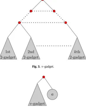
S1 (the tree

agrees with g). Consider the tree in Fig. 2, which we refer to as theith 2-gadget.

Fig. 2.2-gadget.

Fig. 3.v-gadget.

Fig. 4.v-gadget∗.

With respect to this tree,bwins a tournament Tv

∈

S iffvi

=

j. Indeed, ifvi

=

j, thenxijTvbTvx1i−j, and in particularb

beatsx1_i−j; ifvi

=

j, then x1i−jTvbTvxij, sobloses tox 1−j i .

Letv

∈ {

0

,

1

}

k. We will now use the 2-gadget to build a tree wherebwins only the tournamentTv

∈

S, and loses every

other tournament in S. Consider a balanced tree such that the deepest nodes in the tree are in fact 2-gadgets (as in Fig. 3).

As before,bwins in theith 2-gadget iffvi

=

j. We will refer to this tree as av-gadget.

Now, notice that if b wins in each of the 2-gadgets (and this is the case in the tournament Tv), thenb is the winner

of the entire election. On the other hand, let v

=

v, i.e., there existsi

∈ {

1

, . . . ,

k

}

such that w.l.o.g. 0

=

v_i

=

vi

=

1. Then

it holds thatx0_iTvbTvxi1; this implies thatx0i wins in theith 2-gadget.x0i proceeds to win the entire election, unless it is

beaten in some stage by some other alternativex_lj—but this must be also an alternative that beatsb, as it survived thelth

2-gadget. In any case,b cannot win the election.

Consider the small extension, in Fig. 4, of the v-gadget, which (for lack of a better name) we call thev-gadget∗.

Recall that, in every tournament in S,abeats any alternative xi_j but loses to b. Therefore, by our discussion regarding

the v-gadget, b wins the election described by the v-gadget∗ only in the tournamentTv; for any other tournament in S,

alternativea wins the election.

We now present a tree and prove that it is as required, i.e., in any tournament in S1, b is the winner, and in any

tournament in S

\

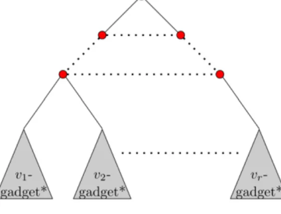
S1,aprevails. Let us enumerate the tournaments in S1:

S1

= {

Tv1

, . . . ,

Tvr

}

.

We construct a balanced tree, as in Fig. 5, where the bottom levels consist of thevl-gadgets*, forl

=

1

, . . . ,

r.

LetTvl

∈

S1. What is the result of this tournament in the election described by this tree? First, note thatbprevails in the

vl-gadget∗. The only alternatives that can reach any level above the gadgets areaandb, andb always beatsa. Therefore,

b proceeds to win the election. Conversely, let Tv

∈

S

\

S1. Then a survives in every vl-gadget∗, forl

=

1

, . . . ,

r.a surely

proceeds to win the entire election.

We have shown that

V

m shattersS, thus completing the proof.

2

Remark 4.2. Even if we restrict our attention to the class of balanced voting trees (corresponding to a playoff schedule),

the dimension of the class is still exponential inm. Indeed, any unbalanced tree can be transformed to an identical (as a

voting rule) balanced tree. If the tree’s height ish, this can be done by replacing every leaf at depthd

<

h, labeled by an

alternativea, by a balanced subtree of heightd

−

hin which all the leaves are labeled bya. This implies that the class of

balanced trees can shatter any sample which is shattered by

V

m.

Remark 4.3.The proof we have just completed, along with Lemma 2.4, imply that the number of different pairwise voting

Fig. 5.The constructed tree.

Theorem 4.1, coupled with Theorem 2.6, implies that the sample complexity of learning arbitrary voting trees is

expo-nential innandm.

4.2. Small voting trees

In the previous section, we have seen that in general, a large number of examples is needed in order to learn voting trees in the PAC model. This result relied on the number of leaves in the trees being exponential in the number of alternatives. However, in many realistic settings one can expect the voting tree to be compactly represented, and in particular one can

usually expect the number of leaves to be at most polynomial inm. Let us denote by

V

m(k)the class of voting trees overm

alternatives, with at mostkleaves. Our goal in this section is to prove the following theorem.

Theorem 4.4.DG

(

V

m(k)

)

=

O

(

klogm

)

.

This theorem implies, in particular, that if the number of leaves k is polynomial inm, then the dimension of

V

m(k) is

polynomial inm. In turn, this implies by Lemma 2.5 that the sample complexity of

V

m(k)is only polynomial inm. In other

words, there is a polynomial p

(

m

,

1

/

,

1

/δ)

such that, given a training set of size p

(

m

,

1

/

,

1

/δ)

, any algorithm that returns some tree consistent with the training set is an

(

, δ)

-learning algorithm for

V

m(k).

To prove the theorem, we require the following straightforward lemma. Lemma 4.5.

|

V

m(k)

|

k

·

mk

·

Ck−1, where Ckis the kth Catalan number, given by

Ck

=

1 k

+

1

2k k

.

Proof. The number of voting trees with exactlykleaves is at most the number of binary tree structures multiplied by the

number of possible assignments of alternatives to leaves. The number of assignments is clearly bounded bymk_{. Moreover,}

it is well known that the number of rooted ordered binary trees withkleaves is the

(

k

−

1

)

Catalan number. So, the total

number of voting trees with exactlykleaves is bounded bymk

·

Ck−1, and the number of voting trees withat most kleaves

is at mostk

·

mk

·

_C k−1

.

2

We are now ready to prove Theorem 4.4. Proof of Theorem 4.4. By Lemma 4.5, we have that

V

(k) m

k

·

mk

·

Ck−1

.

Therefore, by Lemma 2.4: DG

V

(k) m

log

V

m(k)

=

O

(

klogm

).

2

4.3. Computational complexity

In the previous section, we restricted our attention to voting trees where the number of leaves is polynomial ink. We

class is polynomial inm. Therefore, any algorithm that is consistent with a training set of polynomial size is a suitable learning algorithm (Theorem 2.5).

It seems that the significant bottleneck, especially in the setting of automated voting rule design (finding a compact representation for a voting rule that the designer has in mind), is the number of queries posed to the designer, so in this regard we are satisfied that realistic voting trees are learnable. Nonetheless, in some contexts we may also be interested in computational complexity: given a training set of polynomial size, how computationally hard is it to find a voting tree which is consistent with the training set?

In this section we explore the above question. We will assume hereinafter that the structure of the voting tree is known

a priori. This is an assumption that we did not make before, but observe that, at least for balanced trees, Theorems 4.1 and 4.4 hold regardless. We shall try to determine how hard it is to find an assignment to the leaves which is consistent

with the training set. We will refer to the computational problem asTree-SAT(pun intended).

Definition 4.6. In the Tree-SAT _{problem, we are given a binary tree, where some of the leaves are already labeled by}

alternatives, and a training set that consists of pairs (Tj,xij), whereTj

∈

T

andxij

∈

A. We are asked whether there exists

an assignment of alternatives to the rest of the leaves which is consistent with the training set, i.e., for all j, the winner in

Tj with respect to the tree isxij.

Notice that in our formulation of the problem, some of the leaves are already labeled. However, it is reasonable to expect

any efficient algorithm that finds a consistent tree, given that one exists, to be able to solve theTree-SAT_{problem. Hence,}

an

N P

-hardness result implies that such an algorithm is not likely to exist.

Theorem 4.7.Tree-Satis

N P

-complete.

Proof. It is obvious thatTree-SAT is in

N P

. In order to show

N P

-hardness, we present a reduction from 3SAT. In this

problem, one is given a conjunction of clauses, where each clause is a disjunction of three literals. One is asked whether

the given formula has a satisfying assignment. It is known that 3SATis

N P

-complete [11].

Given an instance of 3SATwith variables

{

x1

, . . . ,

x_m

}

, and clauses

{

lj 1

∨

l j 2

∨

l j 3

}

k

j=1, we construct an instance ofTree-Sat

as follows: the set of alternatives is

A

= {

a

,

b

,

x1

,

¬

x1

,

c1

,

x2

,

¬

x2

,

c2

, . . . ,

xm

,

¬

xm

,

cm

}

.

For each clause j, we define a tournamentTj as some tournament that satisfies the following restrictions:

1. l₁j,l₂j andl₃j beat any other alternative among the alternativesxi

,

¬

xi, possibly excluding their own negations.

2. aloses tol₁j,l₂j andl₃j, but beats any other alternative among the alternativesxi

,

¬

xi.

In addition, all tournaments in our instance ofTree-SATsatisfy the following conditions:

1. bbeats any alternative which corresponds to a literal, but loses toa.

2. For alli

=

1

, . . . ,

m,

¬

xi beatsxi.

3. ciloses toxi and

¬

xi, and beats any other literal and the alternativesa andb. The tournaments are arbitrarily defined

with respect to competitions betweenciandck,i

=

k.

Finally, for each tournament, we require the winner to be alternativeb. We now proceed to construct the given (partially

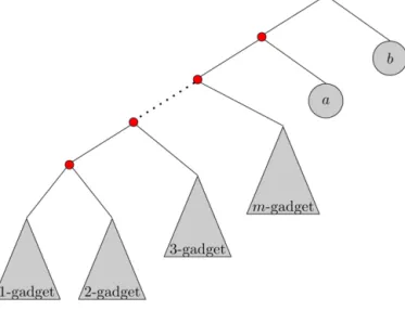
assigned) tree. We start, as in the proof of Theorem 4.1, by defining a gadget which we call ani-gadget, illustrated in Fig. 6.

In this subtree, two leaves are already assigned withxi andci. Now, with respect to any of the tournaments we defined,

if we assign

¬

xi to the last leaf, then

¬

xi proceeds to beatci, and subsequently beatsxi. If we assign xi to the third leaf,

then xi beats ci and wins the election. If we assign any other alternative that is notck for somek

=

1

, . . . ,

m, then that

alternative is defeated byci, which in turn is beaten by xi. Finally, ifck is assigned, it either loses toci and thenxi is the

winner, or it beatsciand proceeds to beatxi. To conclude the point, eitherxi,

¬

xi, orckfor somek

=

i survive thei-gadget.

Using thei-gadgets, we design a tree that will complete the construction of ourTree-SATinstance; the tree is described

in Fig. 7.

Fig. 7.The reduction.

We now prove that this is indeed a reduction. We first have to show that if the given 3SATinstance is satisfiable, there

is an assignment to the leaves of our tree (in particular, choices of xi or

¬

xi) such that, for each of them tournaments,

the winner is b. Consider some satisfying assignment to the 3SAT instance. For every literal l_i that is assigned a truth

value, we assign the labelli to the unlabeled leaf of thei-gadget, i.e., we makelisurvive thei-gadget. Now, consider some

tournament Tj. At least one of the literals l₁j, l₂j or l₃j must be true; as these three literals beat all other literals in the

tournament Tj, one of these three literals reaches the competition versusa, and wins; subsequently, this literal loses to

alternativeb. Therefore,b is the winner of the election. Since this is true for any j

=

1

, . . . ,

m, we have that the assignment

is consistent with the given tournaments.

In the other direction, consider an instance of 3SAT_{which is not satisfiable, and fix some assignment to the leaves of the}

tree. A first case that we consider is that under this assignment,cksurvives somei-gadget,i

=

k.ckcannot be beaten on the

way to the root of the tree, except by anothercalternative. Hence,bdoes not win in any of the constructed tournaments.

A second case to consider is that for eachi-gadget, eitherxi or

¬

xisurvives. The corresponding assignment to the 3SAT

instance is not satisfying. Therefore, there is some jsuch thatl₁j

,

l₂j

,

andl₃j are all false. This implies that inTjsome other

literal other than these three reaches the top of the tree to compete againsta, and loses. Subsequently,acompetes against

b and wins, makingathe winner of the election with respect to tournament Tj. Hence, this is not an assignment which is

consistent with all tournaments—but this is true with respect to any such assignment.

2

Despite Theorem 4.7, it seems that in practice, solving theTree-Sat_{problem is sometimes possible; we shall empirically}

demonstrate this.

Our simulations were carried out as follows. Given a fixed tree structure, we randomly assigned alternatives (out of a pool of 32 alternatives) to the leaves of the tree. We then used this tree to determine the winners in 20 random tournaments over our 32 alternatives. Next, we measured the time it took to find some assignment to the leaves of the tree (not necessarily the original one) which is consistent with the training set of 20 tournaments. We repeated this procedure 10 times for each number of leaves in

{

4

,

8

,

16

,

32

,

64

}

, and took the average of all ten runs.

The problem of finding a consistent tree can easily be represented as a constraint satisfaction problem, or in particular as a SAT problem. Indeed, for every node, one simply has to add one constraint per tournament which involves the node and its two children. To find a satisfying assignment, we used the SAT solver zChaff. The simulations were carried out on a PC with a Pentium D (dual core) CPU, running Linux, with 2 GB of RAM and a 2.8 GHz clock speed.

We experimented with two different tree structures. The first is seemingly the simplest—a binary tree which is as close

to a chain as possible, i.e., every node is either a leaf, or the parent of a leaf; we refer to these trees as caterpillars. The

second is intuitively the most complicated: a balanced tree. Notice that, given that the number of leaves is k, the number

of nodes in both cases is 2k

−

1. The simulation results are shown in Fig. 8.

In the case of balanced trees, it is indeed hard to find a consistent tree. Adding more sample tournaments would add even more constraints and make the task harder. However, in most elections the number of alternatives is usually not above several dozen, and the problem may still be solvable. Furthermore, the problem is far easier with respect to caterpillars (even though the reduction in Theorem 4.7 builds trees that are “almost caterpillars”). Therefore, we surmise that for many tree structures, it may be practically possible (in terms of the computational effort) to find a consistent assignment, even when the input is relatively large, while for others the problem is quite computationally hard even in practice.

Fig. 8.Time to find a satisfying assignment.

5. On learning voting rules “close” to target rules

Heretofore, we have concentrated on learning voting rules that are known to be either scoring rules or voting trees. In particular, we have assumed that there is a scoring rule or a voting tree that is consistent with the given training set.

In this section, we push the envelope by asking the following question: given examples that are consistent with some general voting rule, is it possible to learn a scoring rule or a small voting tree that is “close” to the target rule?

Mathematically we are actually asking whether there exist target voting rules f∗ such that minf_α∈Sn

merr

(

fα

)

, or

minf_∈Vm∗err

(

f

)

, is large. This of course depends on the underlying distribution D. In the rest of this section, the implicit

assumption is thatD is the simplest nontrivial distribution over profiles, namely the uniform distribution. Nevertheless, the

uniform distribution usually does not reflect real preferences of voters; this is an assumption we are making for the sake of analysis. In light of this discussion, the definition of distance between voting rules is going to be the fraction of preference profiles on which the two rules disagree.

Definition 5.1.A voting rule f:

L

N

→

_{A is ac-approximation of a voting rule g iff f and g agree on a c-fraction of the}

possible preference profiles:

N

∈

L

N_{: f}

N

=

_g

N

_c

·

(

m

!

)

n

.

In other words, the question is: given a training set

{

(

N_k

,

f

(

N_j

)

}

k, where f:

L

N

→

A is some voting rule, how hard is

it to learn a scoring rule or a voting tree thatc-approximates f, forc that is close to 1?

It turns out that the answer is: it is impossible. We shall first give an extreme example for the case of scoring rules. Indeed, there are voting rules that disagree with any scoring rule on almost all of the preference profiles; if the target rule

f is such a rule, it is impossible to find, and of course impossible to learn, a scoring rule that is “close” to f.

In order to see this, consider the following voting rule that we call flipped veto: each voter awards one point to the

alternative it ranks last; the winner is the alternative with the most points. In addition, ties are broken according to the

lexicographic order on alternative names. This rule is of course not reasonable as a preference aggregation method, but still—it is a valid voting rule.

Proposition 5.2.Let fαbe a scoring rule that is a c-approximation of flipped veto. Then c

1

/

m. Proof. Let

N _{be a preference profile such that f}

α

(

N

)

=

flipped veto

(

N

)

=

x∗, for some x∗

∈

A. Define a set BN

⊆

L

N

as follows: each profile in the set is obtained by switching the place of an alternative x

∈

A, x

=

x∗, with the place of x∗,

in the ordering of each voter that did not rankx∗ last.8 For a preference profile

N₁

∈

BN that was obtained by switching

x withx∗, it holds that the winner under flipped veto is x∗, since its score did not decrease as a result of the switches,

while its situation in terms of tie-breaking remained the same (that is, its name did not change). In addition, under f_α the

situation ofxin

N

1, with respect to score and tie-breaking, is at least as good as the situation ofx∗in

N (voters that have

not switched the two alternatives are ones that rank x∗ last, and the score of the other alternatives remains unchanged).

8 _{It cannot be the case that all voters rankedx}∗_{last, by our tie-breaking assumption with respect to f}

Note that it might be the case thatxandx∗ have the same score under

N₁; however, since flipped veto

(

N

)

=

x∗ it holds

that x∗ is ranked last by at least one voter in

N_{, and hence in f}

α

(

1N

)

ties between xandx∗ are broken in favor ofx. It

follows that fα

(

1N

)

=

x. Therefore, for any preference profile in BN, f_α and flipped veto do not agree.

We claim that for any two preference profiles

₁N and

N₂ on which f_α and flipped veto agree, it holds that BN

1

∩

BN

2

= ∅

. Indeed, assume that there exists

N

∈

_B

N

1

∩

B2N. Assume first that the winner in both profiles isx

∗_{. It cannot be}

the case that the same alternative was switched withx∗ in order to obtain

N from both

₁N and

N₂—that would imply

N 1 and

N

2 are identical. Therefore, assume w.l.o.g. thatx1was switched withx∗ in

N

1 (only in the rankings of voters that

did not rankx∗ last), andx2 was switched withx∗in

₂N. But this means that bothx1andx2are winners in

N under fα

(by the fact thatx∗ was a winner in both

₁N and

N₂)—a contradiction.

In addition, in any two preference profiles

₁N and

N₂ such that

f_α

₁N

=

flipped veto

N₁

=

x∗

,

and

f_α

₂N

=

flipped veto

N₂

=

x∗∗

,

it holds that BN

1

∩

B2N

= ∅

, as flipped veto electsx

∗ _{in all profiles inB} N 1, but electsx ∗∗_{in all profiles in B} N 2.

It follows that for every preference profile on which f_α and flipped veto agree, there are at leastm

−

1 distinct profiles

on which the two voting rules disagree; this proves the proposition.

2

We shall now formulate our main result for this section. The theorem states that almost every voting rule cannot be

approximated by a factor better than 1₂ by any small family of voting rules. We shall subsequently see that the theorem

holds for small voting trees as well as scoring rules.

Theorem 5.3.Let

R

n_mbe a family of voting rules of size exponential in n and m, and let

, δ >

0. For large enough values of n and m, at least a

(

1

−

δ)

-fraction of the voting rules f:

L

n

→ {

_x

1

, . . . ,

xm

}

satisfy the following property:no voting rule in

R

mn is a

(

1

/

2

+

)

-approximation of f .

Proof. We will surround each voting rule f

∈

R

n

m with a “ball” B

(

f

)

, which contains all the voting rules for which f is a

(

1

/

2

+

)

-approximation. We will then show that the union of all these balls covers at most a

δ

-fraction of the set of the

space of voting rules. This implies that for at least a

(

1

−

δ)

-fraction of the voting rules, no scoring rule is a

(

1

/

2

+

)

-approximation.

For a given f, what is the size of B

(

f

)

? As there are

(

m

!

)

n possible preference profiles, the ball contains rules that do

not agree with f on at most

(

1

/

2

−

)(

m

!

)

n preference profiles. For a profile on which there is disagreement, there arem

options to set the image under the disagreeing rule.9Therefore,

B

(

f

)

(

m

!

)

n

(

1

/

2

−

)(

m

!

)

n

m(1/2−)(m!)n

.

(12)

How large is this expression? Let B

(

f

)

be the set of all voting rules that disagree with f on exactly

(

1

/

2

+

)(

m

!

)

n

preference profiles. It holds that

B

(

f

)

=

(

m

!

)

n

(

1

/

2

+

)(

m

!

)

n

(

m

−

1

)

(1/2+)(m!)n

=

(

m

!

)

n

(

1

/

2

−

)(

m

!

)

n

(

m

−

1

)

1+2

1/2(m!) n

(

m

!

)

n

(

1

/

2

−

)(

m

!

)

n

m1/2(m!)n

,

(13)

where the last inequality holds for a large enoughm. But since the total number of voting rules,m(m!)n_{, is greater than the}

number of rules in B

(

f

)

, we have:

m(m!)n B

(

f

)

B

(

f

)

B

(

f

)

₍m!)n (1/2−)(m!)n

m1/2(m!)n

₍m!)n (1/2−)(m!)n

m(1/2−)(m!)n

=

m (m!)n

.

(14) Therefore B

(

f

)

m (m!)n m(m!)n

=

m( 1−)(m!)n

.

₍₁₅₎

If the union of balls is to cover at least a

δ

-fraction of the set of voting rules, we must have

|

R

nm

| ·

m(1−)(m!)

n

δ

·

m(m!)n;

equivalently, it must hold that

|

R

n

m

|

δ

·

m(m!)

n

. However, by the assumption

|

R

n

m

|

is only exponential innandm(rather

than double exponential), so for large enough values ofnand