Performance analysis of frequency shift
estimation techniques in Brillouin distributed
fiber sensors
S
HAHNAM H
ANEEF,
1Z
HISHENGY
ANG,
2L
UCT
HÉVENAZ,
2D
EEPAV
ENKITESH,
1 ANDB
ALAJIS
RINIVASAN1,*1Department of Electrical Engineering, Indian Institute of Technology, Madras, Chennai, 600036, India 2EPFL Swiss Federal Institute of Technology, Institute of Electrical Engineering, SCI STI LT, Station 11, CH-1015 Lausanne, Switzerland
Abstract: The performance of post-processing techniques carried out on the Brillouin gain spectrum to estimate the Brillouin frequency shift (BFS) in standard Brillouin distributed sensors is evaluated. Curve fitting methods with standard functions such as polynomial and Lorentzian, as well as correlation techniques such as Lorentzian Cross-correlation and Cross Reference Plot Analysis (CRPA), are considered for the analysis. The fitting procedures and key parameters for each technique are optimized, and the performance in terms of BFS uncertainty, BFS offset error and processing time is compared by numerical simulations and through controlled experiments. Such a quantitative comparison is performed in varying conditions including signal-to-noise ratio (SNR), frequency measurement step, and BGS truncation. It is demonstrated that the Lorentzian cross-correlation technique results in the largest BFS offset error due to truncation, while exhibiting the smallest BFS uncertainty and the shortest processing time. A novel approach is proposed to compensate such a BFS offset error, which enables the Lorentzian cross-correlation technique to completely outperform other fitting methods.
© 2018 Optical Society of America under the terms of theOSA Open Access Publishing Agreement
OCIS codes:(060.2310) Fiber optics; (060.2370) Fiber optics sensors; (290:5900) Scattering, stimulated Brillouin; (190.4370) Nonlinear optics, fibers.
References and links
1. T. Kurashima, T. Horiguchi, and M. Tateda, “Distributed-temperature sensing using stimulated Brillouin scattering in optical silica fibers,” Opt. Lett.15(18), 1038–1040 (1990).
2. T. Horiguchi, K. Shimizu, T. Kurashima, M. Tateda, and Y. Koyamada, “Development of a distributed sensing technique using Brillouin scattering,” J. Lightwave Technol.13(7), 1296–1302 (1995).
3. M. Nikles, L. Thévenaz, and P. Robert, “Brillouin gain spectrum characterization in single-mode optical fibers,” J. Lightwave Technol.15(10), 1842–1851 (1997).
4. A. Motil, A. Bergman, and M. Tur, “State of the art of Brillouin fiber-optic distributed sensing,” Opt. Laser Technol.
78, Part A, 81–103 (2016).
5. M. A. Soto, and L. Thévenaz,“Modeling and evaluating the performance of Brillouin distributed optical fiber sensors,” Opt. Express21(25), 31347–31366 (2013).
6. A. López-Gil, M. Soto, X. Angulo-Vinuesa, A. Dominguez-Lopez, S. Martín-López, L. Thévenaz, and M. González-Herráez, “Evaluation of the accuracy of BOTDA systems based on the phase spectral response,” Opt. Express24(15), 17200–17214 (2016).
7. A. W. Brown, M. D. DeMerchant, X. Bao, and T. W. Bremner,“Spatial resolution enhancement of a Brillouin-distributed sensor using a novel signal processing method,” J. Lightwave Technol.17(7), 1179 (1999).
8. C. Li, and Y. Li, “Fitting of Brillouin spectrum based on LabVIEW,” in 5th International Conference on Wireless Communications, Networking and Mobile Computing(IEEE, 2009) 1-4.
9. G. P. Agrawal,Nonlinear Fiber Optics, 2nd ed. (Academic, 1995).
10. A. Villafranca, J. A. Lázaro, I. Salinas, and I. Garcés, “Stimulated Brillouin scattering gain profile characterization by interaction between two narrow-linewidth optical sources,” Opt. Express13(19), 7336–7341 (2005).
11. C. Kanzow, N. Yamashita, and M. Fukushima, “Levenberg−Marquardt methods with strong local convergence properties for solving nonlinear equations with convex constraints,” Comput. Appl. Math.172, 375–397 (2004). 12. C. Zhang, Y. Yang, and A. Li, “Application of Levenberg-Marquardt algorithm in the Brillouin spectrum fitting,”
Proc. SPIE7129, 71291Y (2008).
#325297 https://doi.org/10.1364/OE.26.014661
13. Y. Zhang, D. Li, X. Fu, and W. Bi, “An improved Levenberg−Marquardt algorithm for extracting the Features of Brillouin scattering spectrum,” Meas. Sci. Technol.2(1), 015204 (2013).
14. L. Zhao, Y. Li, and Z. Xu, “A fast and high accurate initial values obtainment method for Brillouin scattering spectrum parameter estimation,” Sensor. Actuat. A-Phys.210, 141–146 (2014).
15. Y. Zhang, G. Fu, Y. Liu, W. Bi, and L. Weihong, “A novel fitting algorithm for Brillouin scattering spectrum of distributed sensing systems based on RBFN networks,” Optik124(8), 718–721 (2013).
16. M. A. Farahani, E. Castillo-Guerra, and B. G. Colpitts, “Accurate estimation of Brillouin frequency shift in Brillouin optical time domain analysis sensors using cross correlation,” Opt. Lett.36(21), 4275–4277 (2011).
17. M. A. Farahani, E. Castillo-Guerra, and B.G. Colpitts, “A detailed evaluation of the correlation-based method used for estimation of the brillouin frequency shift in BOTDA sensors,” IEEE Sens. J.13(12), 4589–4598 (2013). 18. S. M. Haneef and K. Srijith, D. Venkitesh and B. Srinivasan, “Accurate determination of Brillouin frequency based
on cross recurrence plot analysis in Brillouin distributed fiber sensor,” in25th International Conference on Optical Fiber Sensors, 103239M (2017).
19. O. L. Bot, J. I. Mars, C. Gervaise, and Y. Simard,“Cross recurrence plot analysis based method for tdoa estimation of underwater acoustic signals,” in Proceedings of 6th International Workshop on Computational Advances in Multi-Sensor Adaptive Processing (IEEE,2015)
20. O. L. Bot, Mars, J. I. Mars and C. Gervaise, “Similarity matrix analysis and divergence measures for statistical detection of unknown deterministic signals hidden in additive noise,” Phys. Lett. A379(40), 2597–2609 (2015). 21. F. Wang, W. Zhan, Y. Lu, Z. Yan, and X. Zhang, “Determining the Change of Brillouin Frequency Shift by Using the
Similarity Matching Method,” J. Lightwave Technol.33(19), 4101–4108 (2015).
22. M. Alem, M. A. Soto, M. Tur, and L. Thévenaz, “Analytical expression and experimental validation of the Brillouin gain spectral broadening at any sensing spatial resolution,” in25th International Conference on Optical Fiber Sensors, 103239J (2017).
23. M. Alem, M. A. Soto, and L. Thévenaz, “Analytical model and experimental verification of the critical power for modulation instability in optical fibers,” Opt. Express23(23), 29514–2532 (2015).
24. S. Kanakambaran, R. Sarathi, and B. Srinivasan, “Identification and localization of partial discharge in transformer insulation adopting cross recurrence plot analysis of acoustic signals detected using fiber Bragg gratings,” IEEE T. Dielect. El. In.24(3), 1773– 1780 (2017).
25. A. Dominguez-Lopez, Z. Yang, M. A. Soto, X. Angulo-Vinuesa, S. Martín-López, L. Thévenaz, and M. González-Herráez, “Novel scanning method for distortion-free BOTDA measurements,” Opt. Express 24(10), 10188– 10204 (2016).
26. N. Marwan, M. C. Romano, M. Thiel, and J. Kurths, “Recurrence plots for the analysis of complex systems,” Phys. Rep.438(5), 237–329 (2007).
1. Introduction
Brillouin optical time-domain analysis (BOTDA) can effectively measure physical parameters such as strain or temperature along an optical fiber in a distributed manner [1, 2]. In a standard BOTDA system, the probe wave is amplified/attenuated by a counter-propagating pump pulse through stimulated Brillouin scattering (SBS) effect, and Brillouin gain spectrum (BGS) at each fiber location is reconstructed by scanning the pump-probe frequency offset [3]. The central frequency of each BGS, which is commonly referred to as Brillouin frequency shift (BFS), depends linearly on the change of temperature or strain. The determination of such BFS is typically challenging since the measurement noise superposed on the BGS degrades the signal quality, resulting in a large uncertainty in BFS estimation [4]. Therefore, in order to alleviate the detrimental impact of noise, it is important to apply a post-processing algorithm on each measured local BGS to extract the corresponding BFS information. Several types of post processing techniques are currently used. One of the methods is to fit selected spectral range of the measured BGS with a second order polynomial, since the central section of BGS can be approximated to be a quadratic function [5, 6]. The detailed statistical analysis and the resulted analytical expression demonstrate that the frequency uncertainty in BFS estimation using quadratic fitting technique is determined by the SNR condition, the full width at half maximum (FWHM) of BGS, and the frequency scanning step [5]. A viable alternative to this technique is the Lorentzian fitting [7, 8], which exploits the fact that the entire measured BGS is expected to be close to a Lorentzian shape [3, 9, 10]. Such a fitting technique can be realized using Levenberg-Marquardt (LM) algorithm [11–15], which is a non-linear least square algorithm with good convergence properties, thus ensuring the smallest error in the derived BGS. The
above mentioned fitting techniques require the pre-selection of the spectral range for fitting. This requirement can be eliminated through a Lorentzian cross-correlation technique [16, 17], which is independent of the parameter initialization and can also provide promising performance for BFS estimation [16]. The uncorrelated noise superposed on the measured BGS is averaged out in the cross correlation process, thus enhancing the SNR of the correlation output and the accuracy of BFS estimation. In addition, by performing the operations in Fourier domain, the cross correlation demands smaller computational complexity compared to that of the curve fitting algorithms. More recently, we have proposed and demonstrated another approach called cross recurrence plot analysis (CRPA) for BFS estimation [18], which is based on similarity matching algorithm for extracting signal with deterministic behavior in the presence of additive noise [19–21]. Although the above mentioned post-processing methods have been successfully utilized in Brillouin distributed sensing, the performance comparison between them has not yet been reported. Such study can be helpful to identify an appropriate post-processing algorithm that is capable of accurately estimating the BFS even at relatively low SNR, and preferably with the least processing time. In this paper, we present a quantified analysis of the relative merits for all the above-mentioned post-processing techniques for BFS estimation through both numerical and experimental investigations. We begin with optimizing a set of key parameters for each technique such as the averaging spectral window size and the fitting window size for both quadratic and Lorentzian fitting techniques, as well as the linewidth of the reference BGS in cross correlation based techniques. After that, a comparative investigation is performed in terms of the BFS uncertainty, the systematic BFS bias error and the computation time under different realistic conditions such as low SNR, large frequency scanning step and truncated BGS due to improper frequency measurement range. It is demonstrated that the cross-correlation technique offers the smallest BFS uncertainty and the fastest processing speed, while suffering from the relatively high BFS offset error due to BGS truncation. A solution to compensate for the BFS offset error is proposed and implemented, leading to the cross-correlation technique outperforming all the other techniques.
2. Optimization of techniques for BFS estimation
It is established that the Brillouin unsaturated gain profileg(ν)of Stimulated Brillouin process is Lorentzian in shape and is expressed as,
g(ν)= gB
1+4ν∆νB−νB2
(1)
which is characterized by the Brillouin gain coefficientgB, center frequency (BFS)νBand the FWHM∆νB, typically in the order of a few tens of MHz in silica fibers.
Frequency (GHz)
10.65 10.7 10.75 10.8 10.85
Normalized amplitude (a.u)
0 0.5
1 Measured Brillouin gain spectrum
Lorentzian fit
57 MHz
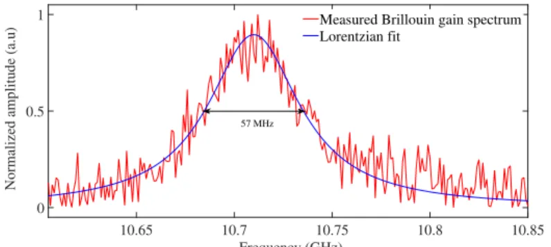
Fig. 1. BGS measured using standard BOTDA setup with 20 ns pump pulses (red trace) and the fit with a Lorentzian profile with a linewidth of 57 MHz.
However, since the measured BGS results from the convolution between the Lorentzian profile of the natural gain spectrum and the normalized power spectral density (PSD) of the pump pulse, both the peak gain and the FWHM of the measured BGS are determined by the characteristics of the pump light, such as the pulse shape and duration. For this reason the BGS may no longer conform to a Lorentzian shape, especially in the case of using a rectangular pump pulse [22]. In our experiment, due to the limited bandwidth of both the electrical pulse generator and the semiconductor optical amplifier (SOA), the generated optical pump pulse reveals a super-Gaussian shape, giving rise to a measured BGS shape close to a Lorentzian profile. As illustrated in Fig.1, the measured BGS (red curve) corresponding to a 20 ns pump pulse fits well to a Lorentzian profile (blue curve) with FWHM of 57 MHz, and such profile will be taken as a reference for all the analysis presented in this work. In a practical scenario, the modulated Brillouin lineshape may not be known apriori. In such cases, we suggest that a sample trace from the initial section of the FUT may be chosen as a reference for further analysis.
In this section, a set of detailed numerical simulations are carried out to optimize the parameters for different BFS estimation techniques, in which an ideal Lorentzian spectrum is considered and different SNR levels ranging from 1 dB to 11 dB are simulated by adding corresponding levels of additive white Gaussian noise (AWGN). Note that here the SNR is defined as the ratio between the maximum amplitude of the BGS and the standard deviation of the signal obtained from consecutive measurements under the same condition. For each SNR value, 1000 different noisy spectra are generated, from which the BFS uncertainty is determined by computing the standard deviation of estimated BFS from the entire set of data.
2.1. Fitting based techniques
2.1.1. Quadratic fitting technique
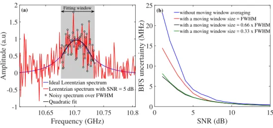
The quadratic fitting is a linear fitting technique and hence is relatively simple [5]. This technique relies on the fact that the central part of the BGS is a Bell-shaped distribution which may be represented as a parabolic function using a limited expansion approximation. Therefore, the BFS νBcan be obtained by fitting a quadratic polynomial to the measured noisy BGS over the FWHM as shown in Fig. 2(a).
10.65 10.7 10.75 10.8 Frequency (GHz) -1 -0.5 0 0.5 1 1.5 2 Amplitude (a.u)
Ideal Lorentzian spectrum
Lorentzian spectrum with SNR = 5 dB Noisy spectrum over FWHM Quadratic fit 0 5 10 15 SNR (dB) 0 5 10 15 20 25 BFS uncertainty (MHz)
without moving window averaging with a moving window size = FWHM with a moving window size = 0.66 x FWHM with a moving window size = 0.33 x FWHM (a) Fitting window (b)
Fig. 2. (a) Simulation results showing a quadratic fit over a sample Lorentzian with SNR = 5 dB, represented by the noisy spectra points (in black circles). The obtained fit curve over FWHM (shaded region) is also shown as black. (b) Comparison of the BFS uncertainty obtained from quadratic fitting using direct peak search and the moving averaging technique with different window size for initial BFS value
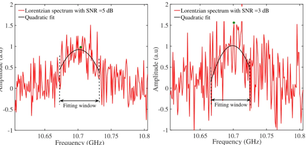
It should be noticed that the quadratic fitting process requires a prior step to determine the initial BFS estimation, which is subsequently used as the center of the spectral window for fitting. We point out that a good symmetry of the fitted quadratic curve (black curve in Fig. 2(a)) within the fitting window is desirable to ensure a good fitting performance, as will be demonstrated hereafter. This imposes a demand of precise selection of the initial BFS, which must be close to the actual BFS. Suffering from the detrimental impact of the noise superposed on the BGS, especially in the case of low SNR, a direct peak search algorithm results in poor fitting performance (12 MHz BFS uncertainty for 3 dB SNR), as shown in blue colour in Fig. 2(b). A wise solution is to apply a moving averaging window on the BGS before performing peak search, thus alleviating the impact of noise. As demonstrated in Fig. 2(b), it is found that the BFS uncertainty obtained after fitting can be massively improved by applying a moving average window with proper size (0.66×FWHM of the BGS). This also indicates that the quadratic fitting technique can reach the optimum performance (i.e., the performance reported in ref. [5]) only when the initial BFS can be precisely estimated. For the sake of visual clarity, Fig. 3 exemplifies the fitted quadratic curves (black ) in cases of 5 dB and 3 dB SNR, respectively. It can be clearly observed that higher the SNR, the more precise of the initial BFS estimation, thus giving rise to more symmetric fitting curve and smaller BFS uncertainty.
10.65 10.7 10.75 10.8 Frequency (GHz) -1 -0.5 0 0.5 1 1.5 2 Amplitude (a.u)
Lorentzian spectrum with SNR =5 dB Quadratic fit 10.65 10.7 10.75 10.8 Frequency (GHz) -1 -0.5 0 0.5 1 1.5 2 Amplitude (a.u)
Lorentzian spectrum with SNR =3 dB Quadratic fit
Fitting window Fitting window
Fig. 3. BFS estimation using quadratic fitting technique for noisy BGS with (a) SNR = 5 dB and (b) SNR = 3 dB. Fitting window selected for each SNR condition is shown for reference and the green dot represents the measured BFS
2.1.2. Lorentzian fitting technique
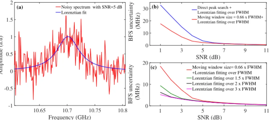
As previously mentioned, since the shape of the experimentally obtained BGS matches well with the Lorentzian profile, the a priori information available (i.e., the Lorentzian function expressed as Eq. (1)) can be utilized for the fitting, which may help in achieving a better performance with respect to quadratic fitting. Figure 4(a) exemplifies a noisy BGS with SNR = 5 dB (red), which is in good agreement with the corresponding Lorentzian fitted curve (blue) obtained through the iterative Levenberg−Marquardt non-linear least squares algorithm.
It should be noted that for the Lorentzian fitting algorithm, the pre-selection of the initial parameters(gB,∆νB, νB)is also of great importance to minimize the BFS uncertainty during the fitting process. Among these parameters, thegBis always set to 1 because the amplitude of the noisy BGS is normalized with respect to the peak value before fitting, and in the case of 2 m spatial resolution the∆νBis selected as 57 MHz [23]. The value of initialνBis estimated following the same procedure for quadratic fitting, in which the moving average process using optimized spectral window size (0.66×FWHM) also helps to improve the fitting performance compared with the direct peak search, as demonstrated in Fig. 4(b). Using the optimized initial parameters, the impact of different fitting window size is compared in Fig. 4(c). The results indicate that in order to obtain a small BFS uncertainty, fitting window size of 3 times larger than the FWHM is desired.
1 3 5 7 9 11 SNR (dB) 0 10 20 BFS uncertainty (MHz)
Moving window size= 0.66 x FWHM +Lorentzian fitting over FWHM Lorentzian fitting over 1.5 x FWHM Lorentzian fitting over 2 x FWHM Lorentzian fitting over 3 x FWHM
10.65 10.7 10.75 10.8 Frequency (GHz) -1 -0.5 0 0.5 1 1.5 2 Amplitude (a.u)
Noisy spectrum with SNR=5 dB Lorenztian fit 1 3 5 7 9 11 SNR (dB) 0 10 20 30 BFS uncertainty (MHz)
Direct peak search + Lorentzian fitting over FWHM Moving window size = 0.66 x FWHM+ Lorentzian fitting over FWHM (b)
(c) (a)
Fig. 4. (a) A noisy BGS with SNR =5 dB (red line) and the corresponding Lorentzian fit (blue line). Green dot represents the actual BFS and the black dot represents the BFS estimated using Lorentzian fitting. (b) BFS uncertainty estimated in different cases of initial BFS estimation. (c) BFS uncertainty estimated using different spectral fitting window size
2.2. Correlation based techniques
2.2.1. Lorentzian cross-correlation technique
Another approach to determine the BFS is based on Lorentzian cross correlation [16, 17]. One of the primary advantages of this approach is that it does not need the procedure of initial BFS estimation before performing the cross-correlation. The key assumption is that the spectral shape is not altered along the sensing fiber, which makes sense for a well-designed BOTDA system. This technique takes the cross correlation between the measured noisy BGS and a reference Lorentzian function, the principle of which is described as following. Letgr(ν)be the normalized reference Lorentzian spectrum:
gr(ν)= 1 1+4ν∆ν−νB Br 2 , (2)
where the spectral linewidth∆νBr should be equal to that of an ideal BGS (57 MHz in this study) in order to obtain the minimum BFS uncertainty [17]. On the other hand, the measured noisy BGSgn(ν)can be expressed as an unperturbed and shifted Lorentzian spectrumg(ν+νs)having the same spectral linewidth, but corrupted with AWGNn(ν)as:
gn(ν)=g(ν+νs)+n(ν), (3)
whereνscorresponds to the shifted BFS owing to changes in temperature/strain. The result of cross correlation (denoted by the ‘∗’ operator) between the reference spectrum and the measured noisy BGS can be described as:
Gr n(ν)=gr(ν) ∗g(ν+νs)+gr(ν) ∗n(ν)=Gc(ν)+Nc(ν), (4) whereGc(ν)is the obtained signal spectrum resulting from the cross-correlation between the two ideal Lorentzian functions (reference spectrum and measured spectrum without noise), which provides an ideal Lorentzian function with a linewidth of∆νB(c) =2∆νB. The other term in Eq. (4),Nc(ν), which represents the cross-correlation between two un-correlated functions (the reference Lorentzian and white noise), would have much lower amplitude than that of termGc(ν),
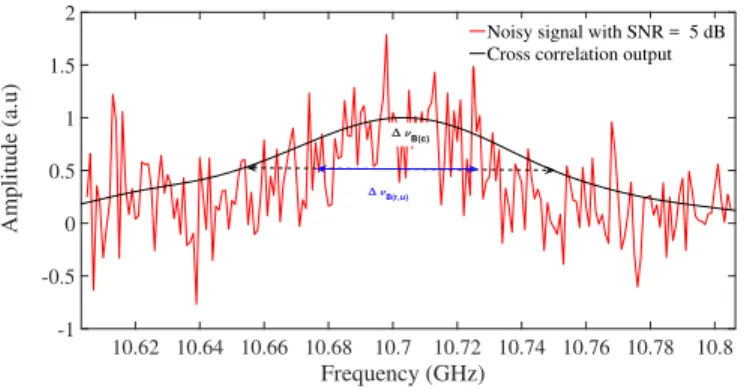
since the cross-correlation of any distribution with a flat white noise spectrum (without any windowing) would result in only a flat spectrum. This way the detrimental impact of noise can be significantly alleviated and hence the value of the BFS can be directly estimated using peak search overGr n(ν). Figure 5 shows an example of using cross-correlation technique for a BGS with 5 dB SNR, where the black curve represents the cross-correlated function.
It is to be emphasised that, in practical cases, a measured BGS from the beginning of the fiber is used as the reference spectrum for the cross correlation technique, which can be a non-Lorentzian due to particular experimental parameters used. Hence the performance of Lorentzian cross-correlation is not affected by a slight deviation in the spectral shape of BGS.
Note that for all the data corresponding to a frequency step of greater than 1 MHz, we have implemented cubic spline interpolation such that we have a data point at every 1 MHz before performing cross correlation to get rid of quantization noise. We have verified that any finer interpolation e.g., 0.1 MHz does not affect at all the BFS uncertainty.
Cross correlation between two signals is normally implemented by a sliding dot product method, which is clearly not ideal in the practical applications due to the high time overhead. In order to accelerate the cross-correlation computation, Fourier transform (FT) property, i.e., the FT of the cross correction between two discrete sequences is identical to the product of conjugate of FT of one sequence with the FT of second series, is used. To take the advantage of this implementation, two correlating functions are represented as two discrete sequences (gr[n] and gn[n], n: sample index) and to find cross correlation, the FT of the two sequences are first calculated and the inverse FT of conjugate product is evaluated. It is well known that the numerical computation is much simpler if the cross correlation product is performed in this manner in the Fourier dual domain.
10.62 10.64 10.66 10.68 10.7 10.72 10.74 10.76 10.78 10.8 Frequency (GHz) -1 -0.5 0 0.5 1 1.5 2 Amplitude (a.u)
Noisy signal with SNR = 5 dB Cross correlation output
B(c)
B(r,u)
Fig. 5. A sample noisy spectrum with SNR of 5 dB (red line) and the (normalized) correlated output (black line)
2.2.2. Cross recurrence plot analysis
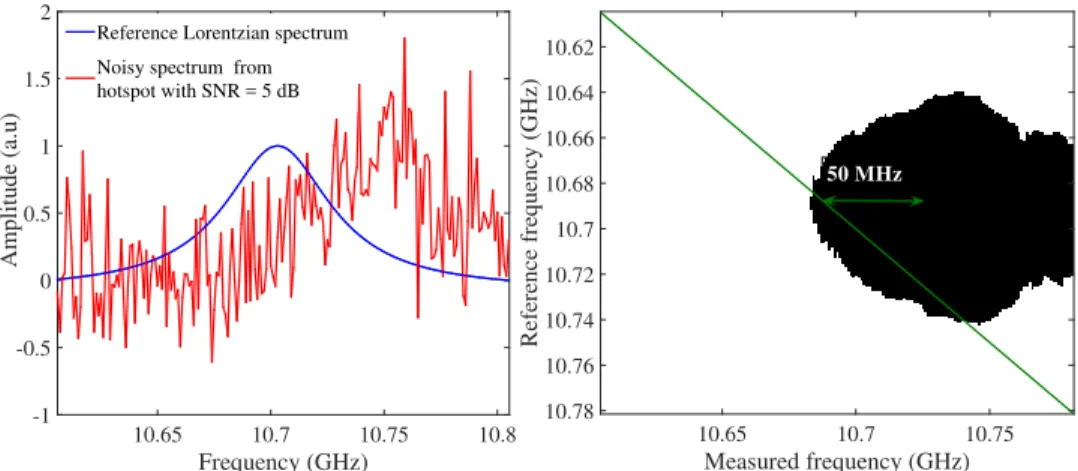
The cross recurrence plot analysis (CRPA) scheme has been previously proposed to track the phase trajectory of deterministic, but dynamic signals by observing the similarity between two time traces. We propose to implement the same to estimate the BFS by computing the cross recurrence between a reference Lorentzian spectrum and the measured noisy BGS.
The CRPA matrix is obtained by computing the similarity (dot product in our case) between the measuredgn(ν)and the referencegr(ν)Lorentzian functions, which have been appropriately delay-embedded to yieldg0n(ν)andg0r(ν). The details of this technique is described in Appendix A. In order to mitigate the effect of noise in the similarity matrix, a threshold corresponding to the standard deviation of the noiseis implemented. The resultant CRPA matrix is expressed as,
C RP A(i,j)=Sim( −−−−→
g0n(ν),
−−−→
Consistent with the above discussion, we chose a reference Lorentzian spectrum with 57 MHz linewidth is taken for the cross recurrence analysis of BGS measured under different SNR conditions.
Figure 6(a) illustrates the reference Lorentzian spectrum (blue line) and a measured spectrum with 5 dB SNR corresponding to a hotspot (shifted by 50 MHz) with SNR of 5 dB. The corresponding CRP matrix is shown in Fig. 6(b). From Fig. 6(b) we can clearly see that the centroid of the similarity patch is shifted with respect to the diagonal line. The diagonal line represents the case where the measured spectrum would be very similar to the reference spectrum (without any frequency shift). Hence, we can directly deduce the BFS by observing the shift in the centroid with respect to the diagonal line. Note that the CRPA technique is also capable of tracking multiple features simultaneously [24], which may be useful when we encounter multi-peak Brillouin spectrum as in the case of LEAF or few mode fibers.
Measured frequency (GHz) 10.65 10.7 10.75 Reference frequency (GHz) 10.62 10.64 10.66 10.68 10.7 10.72 10.74 10.76 10.78 Frequency (GHz) 10.65 10.7 10.75 10.8 Amplitude (a.u) -1 -0.5 0 0.5 1 1.5 2
Reference Lorentzian spectrum Noisy spectrum from hotspot with SNR = 5 dB
50 MHz
Fig. 6. (a) Reference Lorentzian spectrum and measured Brillouin spectrum from a hotspot with SNR of 5 dB and (b) The cross-recurrence plot corresponding to the similarity of the two delay-embedded spectra.
3. Results and discussions
The BOTDA experimental setup is shown in Fig. 7. Light from a narrowband laser is split into two arms to generate both the pulsed pump and the CW probe. The lower branch in the figure shows the generation of the pump, in which a portion of the CW laser light is modulated using semiconductor optical amplifier (SOA) driven by programmable pulse generator (PPG). The peak power of the pulse is boosted by an optical amplifier before launching into the fiber. The upper branch in Fig. 7 shows the generation of the probe using an electro-optic modulator driven by a microwave signal to generate a carrier-suppressed double-sideband CW probe wave. After that, a polarization switch is employed to alleviate the polarization fading effect on Brillouin gain trace. In the receiver part, a Fiber Bragg Grating (FBG) is used before the photo-detector to filter out unwanted spectral components, such as the Rayleigh backscattered light from the pump and the component at the anti-Stokes frequency. Note that the pump and probe power is adjusted to avoid undesirable spectral distortions arising from modulation instability and non-local effects [23, 25].
Fig. 7. Experimental setup of a conventional BOTDA sensor scheme using a pump-probe configuration. SOA: Semiconductor Optical Amplifier, PPG: Programmable Pulse Generator, EDFA: Erbium Doped Fiber Amplifier, TA: Tunable Attenuator, EOM: Electro-Optic Modulator, FUT: Fiber Under Test, PS: Polarization Switch, PD: Photodetector, FBG: Fiber Bragg Grating
In the above experiment, the probe frequency is swept from 10.605 GHz to 10.805 GHz at 1 MHz scanning steps, and 10 sets of data are obtained by performing consecutive measurements in the same condition. The SNR values obtained from the measured data along the 50 km sensing fiber is calculated as ranging from 1 to 11 dB , as shown in Fig. 8(b).
Fig. 8. (a) 3D plot of measured BGS and (b) the SNR values obtained from the measured BGS along the 50 km standard single mode test fiber
3.1. Comparison of performance of the estimation schemes with SNR variations
The experimentally obtained BFS uncertainty profiles are shown as the dots in Fig. 9, which are retrieved with optimized fitting procedure for each technique as described in Section 2. For comparison, the simulation data over 1000 trials for a range of SNR values over 1-11 dB are also illustrated as solid lines. It can be found that the BFS uncertainty computed from the experimental data is quite consistent with the simulation results for all the four estimation techniques considered in our work. In addition, the figure shows that the techniques which use a priori data (corresponding to the Lorentzian function) perform better compared to the quadratic fitting technique. It can be also noticed that the BFS uncertainty scales drastically when the SNR drops below 3 dB, indicating that the measured SNR is preferably maintained above 3 dB to secure a reliable sensing performance.
0 5 10 15 SNR (dB) 0 2 4 6 8 BFS uncertainty (MHz) Quadratic fitting-Simulation Lorentzian fitting-Simulation Lorentzian cross correlation-Simulation CRPA-Simulation
Quadratic fitting-Experiment Lorentzian fitting-Experiment Lorentzian cross correlation-Experiment CRPA-Experiment
Fig. 9. BFS uncertainty based on simulations as well as experimental data for different BFS estimation techniques considered in our work
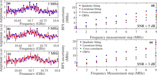
3.2. Performance of estimation schemes with different measurement frequency step
1 2 3 4 5 6 7 8 9
Frequency measurement step (MHz)
2 4 6 8 10 BFS uncertainty (MHz) SNR = 5 dB Quadratic fitting Lorentzian fitting Cross-correlation CRPA 1 2 3 4 5 6 7 8 9
Frequency Measurement step (MHz)
5 10 15 20 BFS uncertainty (MHz) SNR = 3 dB Quadratic fitting Lorentzian fitting Cross-correlation CRPA 10.65 10.7 10.75 10.8 Frequency (GHz) -1 0 1 2 Amplitude (a.u) 3 MHz 10.65 10.7 10.75 10.8 Frequency (GHz) -1 0 1 2 Amplitude (a.u) 5 MHz 10.65 10.7 10.75 10.8 Frequency (GHz) -1 0 1 2 Amplitude (a.u) 7 MHz (c) (a) (b) (e) (d)
Fig. 10. (a-c) Lorentzian spectrum with SNR = 5 dB, measured with a frequency scanning step of 1 MHz over a range from 10.605 GHz to 10.805 GHz (red line) along with the spectrum measured at larger frequency steps of 3 MHz, 5MHz and 7 MHz (blue line) respectively. BFS uncertainty as a function of different frequency scanning step, measured for different schemes for (d) SNR= 5 dB and (e) SNR= 3 dB
In the data considered above, the frequency scanning step is 1 MHz, which leads to relatively long measurement time (in a few minutes), since the typical frequency scanning range spans over a few hundreds of MHz. Enlarging the frequency scanning step can reduce the measurement time, but may also lead to a degradation of BFS uncertainty. In the following validation, for each SNR value the frequency scanning step is varied from 1 MHz to 10 MHz by down-sampling the experimental BGS, as illustrated in Figs. 10(a)-10(c), and the obtained BFS uncertainties in 5 dB SNR and 3 dB SNR are summarized in Figs. 10(d) and 10(e), respectively. It is observed that for all the post-processing techniques the BFS uncertainty gets worse as the frequency scanning step becomes larger, roughly following a square root dependence, which is in good agreement with the study reported in [5]. It can be also seen that the performance of the quadratic fitting technique is always poorer regardless of the frequency scanning step, and the cross-correlation based techniques outperform fitting-based techniques, which is consistent with the results shown in Fig. 9.
3.3. Performance of estimation schemes with truncated BGS
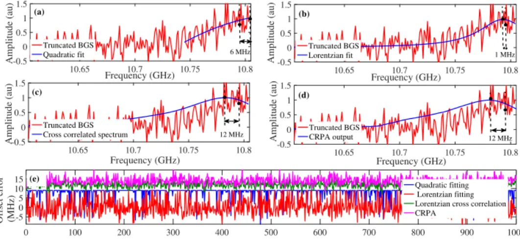
Another common aspect encountered in practical Brillouin sensors is the BFS uncertainty and offset error due to truncation of the measured BGS. This comes from the fact that usually in BOTDA the frequency scanning range is finite, so that the BFS might be spectrally located very close to the edge of the frequency scanning range. Therefore, it is meaningful to investigate the degradation of BFS estimation performance for different post-processing techniques in the case of badly centred BGS (truncated BGS).
10.65 10.7 10.75 10.8 Frequency (GHz) -0.5 0 0.5 1 1.5 Amplitude (au) Truncated BGS Quadratic fit 10.65 10.7 10.75 10.8 Frequency (GHz) -0.5 0 0.5 1 1.5 Amplitude (au) Truncated BGS Lorentzian fit 10.65 10.7 10.75 10.8 Frequency (GHz) -0.5 0 0.5 1 1.5 Amplitude (au) Truncated BGS Cross correlated spectrum
10.65 10.7 10.75 10.8 Frequency (GHz) -0.5 0 0.5 1 1.5 Amplitude (au) Truncated BGS CRPA output 0 100 200 300 400 500 600 700 800 900 1000 -5 0 5 10 15 Offset error (MHz) Quadratic fitting Lorentzian fitting Lorentzian cross correlation CRPA 6 MHz 1 MHz 12 MHz 12 MHz (c) (a) (b) (d) (e)
Fig. 11. (a-d) Demonstration of performance of different BFS estimation techniques for a truncated BGS and (e) the BFS estimated using the these techniques for BGS truncated at a fixed position
A numerical analysis is firstly carried out, in which the frequency scanning range from 10.605 GHz to 10.804 GHz is chosen at 1 MHz scanning step, and the BFS is set to 10.795 GHz as an example, which corresponds to a BGS truncated at BFS+10 MHz. Figures 11(a-d) shows the fitting results using all the four techniques at 5 dB SNR condition. In such a situation the BGS includes only 10 spectral points beyond the BFS, which leads to a larger error in the initial BGS peak search using the moving window averaging technique, thus affecting the performance of quadratic fitting and Lorentzian fitting. Moreover, since the quadratic fitting only makes use of the frequency points within FWHM of BGS, it is not possible to fit a symmetrical quadratic polynomial around the BFS (Fig. 11(a)), which results in an offset error. On the other hand, the Lorentzian fitting utilizes the entire spectral range as the fitting window, hence it shows a better performance in determining the BFS compared to quadratic fitting technique in terms of both offset error and the frequency uncertainty (Fig. 11(b)). Cross-correlation based techniques do not need prior peak search, thereby offering the least BFS uncertainty. However, it is clear that the shift of the cross-correlation peak due to the truncated signal causes larger offset error for BFS estimation (Figs. 11(c) and 11(d)). For the sake of clarity, Fig. 11(e) shows the estimated BFS for 1000 trials using different techniques analysed above. As mentioned before, due to the lack of sufficient frequency points within the FWHM, fitting with a quadratic function turns out to give a semi-parabolic function with a peak close to the last scanning frequency, which results in the estimated BFS to be clipped beyond the maximum offset corresponding to the edge of measurement frequency range.
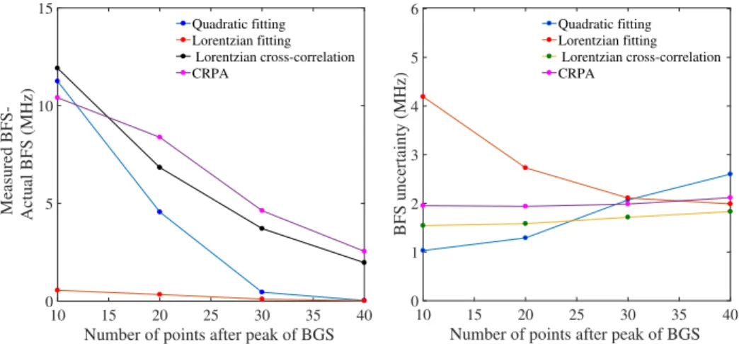
Figures 12(a) and (b) summarizes the performance comparison of different techniques at 5 dB SNR, in which the BFS is also varied from 10.765 GHz to 10.795 GHz with 10 MHz interval, such that the BGS is truncated at BFS+40 MHz, 30 MHz, 20 MHz and 10 MHz, respectively. It can be found that Lorentzian fitting technique results (red points) in the least offset error, while
the BFS uncertainty is the largest. Significantly, the uncertainty for Lorentzian fitting increases for higher levels of truncation (corresponding to smaller number of points after peak of BGS). Incidentally, the Quadratic fitting technique also provides similar uncertainty values but it is not apparent in Fig. 12(b) due to clipping of the values in Fig. 11(e). On the contrary, the BFS uncertainty obtained from the cross-correlation techniques remains almost constant at each level of truncation, but the BFS offset error is far larger than other techniques.
10 15 20 25 30 35 40
Number of points after peak of BGS 0 5 10 15 Measured BFS- Actual BFS (MHz) Quadratic fitting Lorentzian fitting Lorentzian cross-correlation CRPA 10 15 20 25 30 35 40
Number of points after peak of BGS 0 1 2 3 4 5 6 BFS uncertainty (MHz) Quadratic fitting Lorentzian fitting Lorentzian cross-correlation CRPA
Fig. 12. (a) Offset error and (b)BFS uncertainty with BGS spectrum truncated at different positions for SNR = 5 dB
We have investigated the dependence of the offset error on the different levels of truncation as well as SNR for the cross-correlation technique. Note that this systematic BFS offset error as illustrated in Fig. 13(a) is present even for spectra measured with high SNR. As seen from the inset of Fig. 13(a), the offset error remains constant over a wide range of SNR values for different levels of truncation. It is also observed that the offset error grows rapidly when the level of truncation is larger. Figure 13(b) plots the offset error as a function of levels of truncation. This is explained as follows: Let us consider that the Brillouin gain is obtained for frequencies ranging between f1 and f2, and let fp be the BFS estimated from the cross-correlated output. Interestingly, it is found that the relationship between the BFS offset error and the value off2- fp fits well with an exponential profile, as depicted in Fig. 13(b). This relationship has also been validated analytically using Mathematica software.
10.65 10.7 10.75 10.8 Frequency (GHz) 0.2 0.4 0.6 0.8 1 1.2 Normalized amplitude
Reference Lorentzian spectrum Truncated BGS
Cross correlation output
1 3 5 7 9 11 SNR (dB) 5 10 15 Offset error (MHz)
Number of points after peak of BGS
20 25 30 35 40
End frequency - Estimated frequency (MHz)
5 10 15
Offset error (MHz)
Offset error in Cross-correlation Exponential fit
Offset error-Analytical
10 15 20 25 30 35 40
Number of points after peak of BGS
0 5 10 15 Offset error (MHz) Without compensation With compensation 10 20 40 30 Offset error (a) (b) (c)
Fig. 13. (a) Estimated offset error in the cross correlation technique for a truncated BGS. Estimated offset error for different truncation as a function of SNR of measured BGS is shown in inset. (b) The estimated offset error is shown as a function of difference between estimated BFS and the end frequency of scanning range plotted along with the corresponding exponential fit, (c) offset error as a function of the number of points after the actual BFS with and without compensation procedure is shown as a function of the number of points after the actual BFS.
The exponential relationship is repeatable for different SNR cases, and the parameters for the exponential function are the same for a Lorentzian of fixed linewidth. Such predictability offers the distinct possibility of compensating the BFS offset error based on the proximity of the estimated BFS from the end frequency. Specifically, we find that the offset error is significant only when f2- fpis less than 40 MHz i.e., roughly two-thirds of the FWHM of BGS. Under this circumstance, we can compensate for the offset error using the expression:
BFS= fp−Aex p(−c1(f2− fp)),
where A and c1 are constants that can be calibrated for Lorentzian functions of different linewidth. As demonstrated in Fig. 13(c), the offset error present in cross-correlation technique is greatly eliminated after the compensation procedure that utilizes the exponential function obtained above. The analysis has been repeated for Lorentzian profiles of different linewidth and found to be following similar exponential trends with different rate parameters (Fig. 14(a)). These rate parameters of offset error for different linewidth can be pre-calibrated as they show a linear dependence on the rate parameters of the trailing edge of the corresponding Lorentzian. The offset error is estimated for different measurement frequency steps using a Lorentzian of linewidth of 57 MHz and found to maintain the similar exponential function as shown in Fig. 14(b). As mentioned earlier, for frequency scanning step larger than 1 MHz, interpolation is done prior to the cross-correlation process.
15 20 25 30 35 40 45
End frequency - Estimated frequency (MHz)
0 5 10 15 20 Offset error (MHz) 57 MHz 50 MHz 40 MHz 30 MHz 20 25 30 35 40 45 50
End frequency - Estimated frequency (MHz)
0 5 10 15 20 Offset error (MHz) 1 MHz 2 MHz 3 MHz 5 MHz 7MHz 10MHz (a) (b)
Fig. 14. (a) Estimated offset error in the cross correlation technique for a truncated BGS with (a) different linewidth and (b) different frequency scanning step are shown as a function of difference between estimated BFS and the end frequency of scanning range.
Note that the compensation method presented above is aimed at BGS with Lorentzian profiles which are truncated due to improper measurement frequency range. The deformation in the Lorentzian profile such as presence of multi-peak BGS due to spatially non-resolved events, shift in Brillouin peak due to pump depletion and non-local effects, etc are out of scope of the work presented in this paper.
The BFS uncertainty and the processing time of different BFS estimation techniques under different measurement conditions, such as SNR level, frequency scanning step and the truncation due to inappropriate frequency scanning range, are summarized in Table 1. One can find that the BFS uncertainty is smaller for techniques that use a priori information, i.e., the Lorentzian profile of the BGS. Especially for the Lorentzian cross-correlation technique, the BFS uncertainty is the smallest, and since the corresponding computation is performed in the Fourier domain, the processing time is the shortest as well. The results indicate that associating with the BFS offset error compensation, the Lorentzian cross-correlation is the preferable technique to estimate the BFS when the shape of the measured BGS is close to Lorentzian profile.
Table 1. Comparison of performance of BFS estimation techniques for different measurement conditions
Quadratic Lorentzian Lorentzian CRPA
Performance Metrics fitting fitting correlation
BFS uncer-tainty ( MHz) due to SNR 3 dB 3.86 3.01 2.94 2.71 5 dB 2.29 1.63 1.63 1.80 different scanning step at SNR=3 dB 2 MHz 5.85 4.57 4.02 3.75 4 MHz 9.64 7.12 5.97 5.50 different truncation at SNR=3 dB 10 MHz 4.39 5.58 1.98 2.73 20 MHz 6.50 5.02 2.21 2.95
Processing time* ( seconds) 2.9 4.51 0.25 4.19
*Processing time for 1000 trials per SNR. Hardware: Intel Core i3-3210 CPU with 8 GB RAM. Software: Matlab R2016b (Academic License-IIT Madras), OS-Windows7
4. Conclusion
In this paper, we analyze through numerical simulations and experiments the performance of four different post-processing techniques for BFS estimation in BOTDA, including quadratic fitting, Lorentzian fitting, Lorentzian cross-correlation and Cross Recurrence Plot Analysis (CRPA). The optimization of each fitting technique is firstly carried out using numerical simulation. It is pointed out that the performance of both the quadratic fitting and Lorentzian fitting highly depends on the spectral position of the fitting window that centers on the initial estimated BFS. One proper way to find the initial BFS is to apply a moving average procedure with the averaging size of 0.66×FWHM on the raw BGS, followed by a peak search algorithm performed on the smoothed BGS. We also determine that the size of the fitting window is of great importance, and should be equal to FWHM and 3×FWHM for the quadratic fitting and the Lorentzian fitting, respectively. The cross-correlation based techniques do not need the step of initial BFS estimation, and the only important point is the FWHM of the reference Lorentzian function should be the same as the unperturbed BGS at the initial section of the sensing fiber. After optimization, a quantified performance comparison is carried out in terms of the BFS uncertainty, the systematic BFS offset error and the computation time, under different realistic conditions such as low SNR, large frequency scanning step and truncated BGS. It turns out that techniques relying on a priori information about the BGS (i.e., the Lorentzian function) perform better. Specifically, the Lorentzian cross-correlation technique exhibits the smallest BFS uncertainty and needs the shortest processing time, but with the compromise of the largest offset error. It is pointed out that this frequency offset is predictable and hence can be efficiently compensated, which allows to fully make use of the advantage of the Lorentzian cross-correlation technique. Note that all the study performed in this paper is with the BGS having a Lorentzian shape, which results from the pulse shape used in our experiment. Different pulse shape can lead to different BGS profile, which may affect the fitting performance of each fitting technique but can be readily addressed by appropriately choosing the reference spectrum.
5. Appendix A
The CRP Analysis scheme is implemented in a similar manner as previously reported [19, 20, 24], except that the time delay in previous work is substituted by a frequency shift. Letgnbe the measured noisy BGS which can be represented as
gn(ν)=(g(f1),g(f2), ...g(fNg)) (6) First, the frequency space corresponding to the above spectrum is constructed by a frequency-delay embedding technique over a series of vectors given by
−−−−−→ gnm(ν)=[gn(i),gn(i+δ), ...gn(+(m−1)δ)] (7) = g(f1) g(f2) g(f3) . . g(fm) g(f2) g(f3) g(f4) . . g(fm+1) . . . . . . . . g(fN) g(fN+1) g(fN+2) . . g(fNg)
whereiis the sample index corresponding to the scanning frequency range;i =1,2,3, ...N = Ng− (m−1)δ,δis the index corresponding to the frequency step,mis the embedding dimension andNgis the number of samples ofgn,r. Both embedding parameters, the dimensionmand the frequency stepδhave to be chosen appropriately. In our case,δis taken as 1 corresponding to the measurement frequency step and the embedding dimension is taken as 16. Similarly, the
reference spectrum is reconstructed by a series of vectors as −−−−−→
gr m(ν)=[gr(j),gr(j+δ), ...gr(j+(m−1)δ)] (8)
The frequency space constructed above are appropriately repeated to get the matricesg0n(ν)and
g0r(ν)with order ofN2×m.
The test of similarity of the spectra is calculated using a similarity function, calculated on all possible pairs of frequency space to get the similarity matrix as,
d(i,j)=Sim( −−−−→
gn0(ν),
−−−→
g0r(ν)) (9)
whereSimis the function chosen to study the closeness of the vectors. Here, we useddot product
as the similarity function, which is a kind of piece-wise cross-correlation. The CRPA matrix is then obtained with proper thresholding of the similarity matrixd(i,j)and can be expressed as
C RP A(i,j)=Sim( −−−−→
g0n(ν),
−−−→
gr0(ν)) − (10)
wherecorresponds to the threshold set for obtaining the CRPA matrix. Note that the CRPA
matrix is appropriately reshaped toN×Nand Recurrence Quantification analysis (RQA) [26] is used to quantify the similarity between the spectra based on the non-zero entries in the recurrence plot. A commonly used metric for RQA is the SS-metric, which is defined as
SS(ν)= ∞ Í i=1 C RP A(i−ν,i) d(i−ν,i) ∞ Í i=1 C RP A(i+ν,i) d(i+ν,i) (11)
whereis the Hadamard product andνrepresents the diagonal index,ν= 0 corresponds to main diagonal,ν <0 correspond to the diagonals below the main diagonal andν >0 correspond to the diagonals above. The frequency shiftν0can be estimated as the maximum ofSS(ν)matrix. Funding
Sterlite Technologies, LTD, Auranagabad, India; Department of Electronics and Information Technology (DeitY) and the Ministry of Human Resource Development (MHRD), Government of India; The Swiss Commission for Technology and Innovation (Project 18337.2 PFNM-NM).
Acknowledgments