Planning Effective Cellular Mobile Radio Networks
Stephen Hurley
Abstract—This paper deals with the automatic selection and
configuration of base station sites for mobile cellular networks. An optimization framework based on simulated annealing is used for site selection and for base-station configuration. Realistic path-loss estimates incorporating terrain data are used. The configuration of each base station involves selecting antenna type, power con-trol, azimuth, and tilt. Results are presented for several design sce-narios with between 250 and 750 candidate sites and show that the optimization framework can generate network designs with de-sired characteristics such as high area coverage and high traffic capacity. The work shows that cellular network design problems are tractable for realistic problem instances.
Index Terms—Cell planning, heuristics, radio frequency
assign-ment, radio network design.
I. INTRODUCTION
O
NE OF the most important cellular network planning activities is to select a set of sites from a list of candidate sites that have been identified as potential sites by marketing. The selected sites form the basis of a network that must satisfy certain network requirements such as high area coverage and high traffic capacity but that minimize infrastructure cost. The configuration of the selected base stations is also a complex problem and involves choosing among different antenna types, e.g., various directional or omnidirectional antennas, power control, tilt, and azimuth. This paper considers the use of an optimization framework based on simulated annealing for base-station selection and configuration for realistic-sized networks. Previous work has dealt with aspects of this design problem, e.g., [1]–[10], but none has considered the full complexity of the problem, either because they use simpli-fied models—i.e., by only considering base-station selection without base-station configuration—or because they consider relatively small numbers of candidate sites.Another aspect of the design problem is the relationship with the frequency assignment problem, which aims to generate a fre-quency plan that minimizes electromagnetic interference due to the reuse of frequencies in different parts of the network. De-signing cellular radio networks that utilize their allocated fre-quencies effectively and efficiently is a difficult problem, even though the frequency assignment problem itself is well studied; e.g., [11]–[17]. If a radio network is poorly designed, then spec-trum will be wasted and/or the quality of service will be de-graded even if a good frequency assignment algorithm is used.
To produce a well-designed network, the designer needs to take into account several competing factors. For example, cost
Manuscript received February 2, 2000; revised August 13, 2001. This work was supported by the European Union under ESPRIT Project 23243.
The author is with the Department of Computer Science, University of Wales, CF12 3XF Cardiff, U.K. (e-mail: [email protected]).
Publisher Item Identifier S 0018-9545(02)00425-5.
may be reduced by having a few omnidirectional antennas op-erating at full power. This may produce good area coverage and have a small amount of overlap between cells (and hence low in-terference). However, such a network will probably not be able to satisfy the traffic demands within the cell of each antenna. To try and overcome this problem, more antennas are required (perhaps using directional antennas at the same site or additional antennas at different sites). However, this increases the cost, the potential for interference, and hence the difficulty of finding a good frequency assignment. For example, if the network design is used to generate channel separation constraints between pairs of transceivers, then the required separations could have higher values on a poorly designed network relative to a well-designed network. Consequently, frequency assignment algorithms, e.g., [18] and [19], will find assignments that either use a larger range of frequencies than may be necessary (for minimum span assignment) or have a higher number of constraint violations (more interference) in fixed spectrum problems.
The cellular network optimization problem involves de-signing a network using an optimization algorithm that takes into account competing factors. For example, the final network can be optimized for area coverage, traffic capacity, cost, interference (giving consideration to frequency assignment), and handover. Other objectives can be included as necessary.
II. PROBLEMDESCRIPTION A. The Model
The model used is based on models in [20] and [21]. A net-work is defined within a net-working area . Any point in is defined by its Cartesian coordinates. For simplicity, points in are only defined on a grid. Such data we shall refer to as mesh data. Points within where propagation and service informa-tion is available are known as service test points (STPs). These are represented by
where is the total number of service test points in . We represent a typical service test point by , with coordinates
, where and is the height above sea
level. Mesh data are provided, at each service test point, for the following:
1) propagation loss estimates (line-of-sight path loss); 2) service threshold requirement;
3) traffic demand.
Other data, which we shall refer to as engineering data, are provided for the following:
1) a list of candidate sites, i.e., sites where base stations could potentially be located;
TABLE I
TYPICALSERVICETHRESHOLDS
2) candidate site legacy status, i.e., whether it forms part of a preexisting network or not;
3) a list of different antenna types defined by horizontal and vertical radiation patterns as well as transmission gain and loss.
Both the mesh and engineering data are described in more detail below.
1) A Network: Consider a number of candidate sites
where is the total number of candidate sites available. A network is composed of sites chosen from the list of candidate sites . To define a network, we define a configuration where
where, for the th candidate site in , we have (1), shown at the bottom of the page.
Therefore, a network is defined as follows:
where represents an operational (active) site and is the total number of sites selected by the optimization process to be active in the current configuration
.
In cases where an existing network is to be altered to cope with new conditions—e.g., increased capacity require-ments—we denote the preexisting network as the legacy network.
2) Service and Traffic: A network provides a service based upon criteria defined by the network operator. The nature of the expected service for a network defined on is given by , and the values associated with the points in give the ser-vice threshold (in dBm) for the required serser-vice. We represent the service requirement at an STP by . Typical service thresholds are given in Table I and are characterized by the type
Fig. 1. Example STP data map.
Fig. 2. Example traffic demand data map.
of mobile station assumed to be located at the STP (see Sec-tion II-A6).
Also, during operation, the network must satisfy the capacity (traffic) requirements in an efficient way. The expected traffic demand, measured in Erlang, at each is denoted by
.
Fig. 1 shows an example of an STP data map. The darker the shade of gray, the higher the service threshold requirement at the test point. Similarly, Fig. 2 shows an example traffic demand data map, with lighter shades of gray indicating the increasing traffic demand (black indicates zero traffic demand).
if site is not used, i.e., not selected
if site is operational, i.e., it is used (contains at least one base station)
3) A Site: Each operational site consists of one or more base stations (BSs). The model represents a base station by
where (2)
where is the base station of operational site and is the number of base stations at site . For an operational
site, we have .
A candidate site has a geographical position on repre-sented by
where and are the Cartesian coordinates of candidate site and its height above sea level.
The propagation loss from every candidate site to each STP defined on is given by , where
contains estimates of the propagation losses to each STP defined on relative to site , i.e., contains propagation loss estimates (in dB). The propagation model used to generate the line-of-sight path-loss estimates is based on the COST 231 Walfish–Ikagami model [22], [23].
4) A Base Station: In addition to the set of sites, it is possible to consider a set of base stations
where is the total number of operational base stations. Pre-viously, in (2), we defined the operational base station of operation site by ; therefore we have
if
A given base station where , situated at site
, has a number of operational parameters that are variables in the optimization process. These allow the configuration of the base station and include the following:
transmitting power (in dBm) of ;
the antenna type of , i.e., there
are different types of antennas available;
angle of tilt of the antenna of ;
azimuth of the antenna of ;
number of TRX devices (transmitters) used by (this corresponds to the number of channels required by the base station). The traffic capacity (in Erlangs) per TRX is given in Table II1 (see [24]).
5) Antennas: Each base station has one antenna. For the networks presented in the results section (Section V-A), it is assumed that an antenna can be omnidirective, small (narrow) panel directive, or large panel directive; hence . The
1Sometimes an eighth TRX is used, which allows a capacity of 58 Erlang to
be satisfied
TABLE II CAPACITYPERTRX
radiation pattern of an antenna is characterized by two func-tions, which define the horizontal and vertical losses (in dB) depending on the horizontal and vertical angles of the antenna relative to the STP and base station. Therefore, for a given an-tenna type, we define
and
which represent the losses for each angle between 0 and 359 in the horizontal and vertical directions, respectively.
Finally, each antenna has an associated (and fixed) transmis-sion gain and loss (in dB) represented, respectively, as
and
6) Mobile: There are a number of different mobile station types that can be located at a service test point, for example 2 W, 8 W. Each mobile station type has an associated (and fixed) reception gain and loss (in dB) represented, respectively, by
and
The mobile type located at a given service test point is given in the set , i.e., the mobile type is a function of . Therefore, we represent the mobile type at a given service test point by , i.e., the mobile to be serviced at . Note that has an associated service requirement (see Section II-A2 and Table I).
B. Definitions
1) Downlink Field Strength: For a given base station sit-uated at site , the downlink field strength at a service point
is given by
(3) The power of a base station is given in dBm; all other values in (3) are in dB.
2) Cell: A cell is defined for base station as the set of points such that
and
i.e., for all points in cell is the best server (provides the strongest signal).
3) Handover: A necessary feature of a mobile network is the concept of handover, i.e., the ability to transfer responsibility of a mobile signal from one base station to another. The handover set HAND operates on the cell of the base station and is defined as the subset of points in such that the field strength
at received from base station is within 7 dB of the field strength at received from a neighboring base station , i.e.,
HAND and
such that
For a given cell, the handover may be satisfied by more than one base station. Here we set the target number of neighboring base stations satisfying handover for a point HAND to four.
III. DESIGNOBJECTIVES
The objectives of a network design (cell plan) are as follows. 1) Coverage: All service test points receive at least one signal above its service threshold, i.e., for all service points , we require
where
if otherwise
The point is said to be covered if it receives at least one signal above its service threshold.
2) Traffic Capacity: The traffic load within a cell should be less than some maximum value corresponding to the capacity of the maximum number of TRX devices (chan-nels) available. Currently, the value used corresponds to 43 Erlang, the capacity of seven TRX devices (see Table II), i.e., for all cells , we require
A maximum capacity per cell allows us to calculate the theoretical minimum number of sites and base stations that must be active for any network design to satisfy the traffic capacity objective. We define the minimum number of base stations (cells) required by
Therefore, the corresponding theoretical number of sites that must be active is
max cells per site (4)
where max cells per site is the maximum number of base stations that could occupy a single site (three is used throughout this paper).
We should note that in this model, we assume that the traffic at a test point can only be served by the base station that presents the strongest signal at its location. There-fore, the element of choice is eliminated and network ca-pacity is easy to calculate. However, in a protocol such as GSM, a mobile station may choose from a number of base stations whose signal strength is above an accept-able threshold. Therefore, an evaluation in which only the base station with highest signal strength was an accept-able server may give a conservative estimate of network capacity.
3) Site Cost: The number of sites used in the design or their associated financial cost should be minimized, i.e.,
where is the cost associated with site and is de-fined by (1).
4) Handover: Currently, this objective is implemented simply (for computational efficiency rather than network effectiveness) by requiring that each cell should have at at least one service test point in such that
HAND
i.e., there exists at least one service test point such that each signal from four base stations is within 7 dB. The objective is to have as many cells as possible satisfying the handover condition.
5) Interference: This objective attempts to minimize a mea-sure of potential interference in the design. Our meamea-sure is to minimize overlap, i.e., at each service test point , minimize the number of interfering base stations
(5) where
if otherwise
where is the receiver sensitivity (set to 99 dBm). An interfering base station is defined as a base station providing a signal strength at a service test point that is greater than but is not the best server nor one of the base stations providing handover.
IV. THEDESNETFRAMEWORK
DESNET2 incorporates a simulated annealing algorithm
to-gether with problem-specific neighborhood structures. Specific neighborhood structures are used to improve solutions that are deficient in specific areas—for example, coverage or capacity not satisfied. A random neighborhood is also used to diversify the search.
A weighted objective function is used to guide the search to-ward solutions that satisfy the design objectives as well as pos-sible. Typically, elements of the objective function that corre-spond to important objectives in the model (e.g., coverage and capacity) are weighted higher than the lower priority objectives. All customizable aspects of the design algorithm are specified by a list of parameters. Fig. 3 contains the overall optimization framework.
A. Initialization
There are several methods that can be used to initialize a net-work, i.e., generate a starting network.
1) Legacy: The initial network is given by a preexisting de-sign.
2) Partial: The number of sites to be randomly selected in the initial network is specified as a percentage of the the-oretical minimum number of sites required to fulfill the
Fig. 3. DESNETsolution framework.
Fig. 4. SA algorithm.
traffic requirement, i.e., , where .
The actual sites are then randomly configured.
3) Full: A special case of partial initialization, i.e., . 4) Full coverage: The hole filler neighborhood (see
Sec-tion IV-D1) is used until all service points in the network are covered (no other objectives are considered). B. Simulated Annealing Algorithm
A simulated annealing algorithm (see [25]) controls the choice and acceptance of new solutions (network designs). The overall procedure is given in Fig. 4. is the current temperature and random is a uniformly distributed random number in the range [0, 1]. A standard geometric temperature reduction rule is used to lower the temperature parameter, i.e., , and the number of trial networks tested at each temperature is set to 2 .
1) Starting and Finishing Temperatures: The starting tem-perature is determined as follows.
1) Set the initial temperature to 1.0.
2) Examine trial networks and count the number of accepted ones.
3) If the acceptance ratio , which is defined as the number of accepted trials divided by , is less than 0.3, double the temperature.
4) Goto Step 2) until the observed acceptance ratio exceeds 0.3.
The algorithm terminates when the temperature falls below some user-specified minimum temperature , or if the number of frozen temperatures exceeds another user-specified value . A frozen temperature occurs when no new trial networks have been accepted at a given temperature.
The parameters mentioned here for algorithm implementa-tion are largely selected by experimentaimplementa-tion since at present, there are no general rules that guide the choice of annealing pa-rameters. The way they are selected is a matter of experience for the practitioner (see [25] for a detailed discussion).
C. Objective Function
To endeavor to meet the objectives of a network design, the objective function used is a weighted additive objective function (to be minimized) of the form
(6)
where is the cost of component (and includes its associated weight ). The components used in this function are related to the design objectives in Section III and are as follows.
1) Coverage: A normalized cost based on the number of ser-vice test points covered, i.e.,
where is the total number of service test points and is the number of covered service test points in the current network.
2) Site cost: The normalized site cost component in the ob-jective function reflects the relative financial cost of uti-lizing site locations. For a given configuration of sites , the site-cost component for a Greenfield scenario (see Section V) is given by
(7)
where is the financial cost associated with site . If a preexisting network is to be changed and aug-mented, i.e., an expansion scenario (Section V), the site cost component is given by
(8) where is shown in (9) at the bottom of the next page. reflects the relative cost of adding, removing, or changing a site.3
3Figures provided by France Telecom; other operators may attach different
3) Traffic: A normalized cost based on the traffic capacity of the current network relative to the total traffic capacity required, i.e.,
where is the total traffic capacity
required by a network design and
is the traffic capacity of the current network design and reflects the sustainable capacity in the network (any over capacity 43 Erlangs in a cell is discounted).
4) Interference: This cost based on the total interference in the network, normalized by a user-specified scaling factor, is given by
where is the interference of the current network design [see (5)] and is a parameter specifying a maximum interference level for the network (only used for normal-ization in ) and equals the value of obtained when an omnidirectional antenna, at maximum power, is placed at all candidate sites.
5) Handover: A normalized cost based on the proportion of cells satisfying the handover condition, i.e.,
where is the number of cells in the current net-work design that satisfy the handover condition and is the number of base stations in the current network design. D. Neighborhood Structures
Currently, four specific neighborhood structures (move generators) are used to improve solutions in two specific areas of network statistics: coverage and traffic. The usage and preference of each neighborhood is governed by four probabilities. Each neighborhood is only considered if the necessary conditions are present and a random number be-tween zero and one is less than the corresponding probability . Details of this move selection procedure are given in Fig. 5.
Note that the networks formed by applying any of these neighborhood structures are subject to the same acceptance criterion as the random neighborhood (which simply randomly changes any single network characteristic, i.e., turns on or off a site or any aspect of a base station configuration, e.g., assigns a random power to a randomly selected base station).
Fig. 5. Network design procedure.
1) Hole Filler Neighborhood: The hole filler attempts to fill coverage holes in the network. To cover as much of the hole as possible, the site closest to the center of mass4 of the hole is
se-lected (this also can be restricted to the closest active site or the closest inactive site). An omnidirectional antenna is placed at the site (any previous antennas are removed if the site is already active). The power is set to be the smallest value that covers the maximum number of service points of the hole—using a lower-powered antenna helps reduce the interference in the network. Fig. 6 details the operation of the hole-filling move.
The following hole-filler parameters can be used to tune the operation of the neighborhood.
1) HRType: The method used to select the site to be added and selected from:
a) Closest: closest site to center of mass of hole (de-fault);
b) Closest on: closest active site to center of mass of hole;
c) Closest off: closest inactive site to center of mass of hole;
4The “center of mass” of a hole is calculated using the assumption that each
service test point in the hole has unit mass.
if site is not used in the legacy and expanded network if there is no change to site in the legacy network if there is any change on site in the legacy network if site is newly installed
if site is removed from the legacy network.
Fig. 6. Hole filler procedure.
Fig. 7. Cell-splitting procedure.
2) HRPowerMax: Maximum power allowed at the new site (default—55 dBm).
3) HRPowerMin: Minimum power allowed at the new site (default—26 dBm).
4) HRPowerStep: Increment used to vary power at the new site (default—2 dBm).
Note that no azimuth needs to be set as a hole filler always places an omnidirectional antenna.
2) Small Cell Removal: Base stations corresponding to cells whose size, given by the number of STPs it contains, is below a specified size, e.g., ten service points, are removed. Stations that cover no service points are automatically removed.
3) Cell Splitter: The cell-splitter neighborhood (see Fig. 7) aims to improve the traffic capacity of the network by replacing an omnidirectional antenna by three directive antennas at the same site. The azimuth and tilt of the new antennas are chosen
Fig. 8. Traffic filling procedure.
randomly, but the power is taken to be the same as that of the original omnidirectional antenna. This is to try and ensure that the number of service points covered by the new site is at least as many as the original site configuration.
The following cell-splitter parameters are available to tune the operation of the neighborhood:
1) CSAntennaType: the type of directional antenna to be used (default—small directive);
2) CSTilt: the tilt value to be used (default—0 ).
4) Traffic Filler: The traffic filler neighborhood (see Fig. 8) aims to improve traffic capacity by activating a new site within a defined area of the cell violating traffic by the largest amount. The new site is initialized with an omnidirectional antenna and the power is set so that the traffic capacity of the cell is less than 129 Erlang. The cell-splitter neighborhood is then applied to the new site.
Parameters available to tune the traffic filler neighborhood include:
1) TFPowerMax: maximum power allowed at the new site (default—55 dBm);
2) TFPowerMin: minimum power allowed at the new site (default—26 dBm);
3) TFPowerStep: increment used to vary power at the new site (default—2 dBm);
4) TFTilt: tilt to be used for new antenna (default—0 ). Note that the antenna type does not need to be specified as a small directive is always used.
V. DATASETS ANDRESULTS
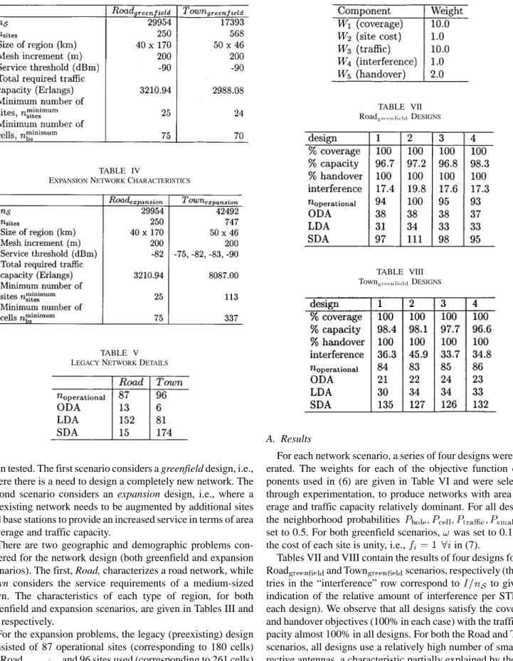
Four real-world data sets have been used for study. All data sets were provided by the CNET5and two design scenarios have
TABLE III
GREENFIELDNETWORKCHARACTERISTICS
TABLE IV
EXPANSIONNETWORKCHARACTERISTICS
TABLE V LEGACYNETWORKDETAILS
been tested. The first scenario considers a greenfield design, i.e., where there is a need to design a completely new network. The second scenario considers an expansion design, i.e., where a preexisting network needs to be augmented by additional sites and base stations to provide an increased service in terms of area coverage and traffic capacity.
There are two geographic and demographic problems con-sidered for the network design (both greenfield and expansion scenarios). The first, Road, characterizes a road network, while Town considers the service requirements of a medium-sized town. The characteristics of each type of region, for both greenfield and expansion scenarios, are given in Tables III and IV, respectively.
For the expansion problems, the legacy (preexisting) design consisted of 87 operational sites (corresponding to 180 cells) for Road and 96 sites used (corresponding to 261 cells) for Town . Full details of the legacy networks are given in Table V (where ODA is number of omnidirectional antenna sectors, LDA is number of large panel directive antennas, and SDA is number of small panel directive antennas).
TABLE VI COSTCOMPONENTWEIGHTS
TABLE VII Road DESIGNS
TABLE VIII Town DESIGNS
A. Results
For each network scenario, a series of four designs were gen-erated. The weights for each of the objective function com-ponents used in (6) are given in Table VI and were selected, through experimentation, to produce networks with area cov-erage and traffic capacity relatively dominant. For all designs,
the neighborhood probabilities are
set to 0.5. For both greenfield scenarios, was set to 0.1, and the cost of each site is unity, i.e., in (7).
Tables VII and VIII contain the results of four designs for the
Road and Town scenarios, respectively (the
en-tries in the “interference” row correspond to to give an indication of the relative amount of interference per STP for each design). We observe that all designs satisfy the coverage and handover objectives (100% in each case) with the traffic ca-pacity almost 100% in all designs. For both the Road and Town scenarios, all designs use a relatively high number of small di-rective antennas, a characteristic partially explained by the set-ting of the CSAntennaType parameter in the cell-splitter neigh-borhood to small directive (see Section IV-D3). The average number of interferers per STP in the Town designs is higher than that in the Road network. This can be explained by the fact that
TABLE IX Road DESIGNS
TABLE X Town DESIGNS
the Road network is axial in nature, i.e., many cells only require a relatively small number of adjoining cells.
Tables IX and X show the designs generated for the two ex-pansion scenarios. For each design, the relevant legacy network is used as the starting network. The rows labeled “changed,” “added,” “removed,” refer to the number of sites changed, added, and removed in the legacy network, respectively; “cost” denotes the cost of these legacy alterations by summing the relevant values for using (9).
The results for the Road expansion problem differ only slightly from the legacy network since the initial network required relatively small improvements in area coverage and capacity (a few percent in each case). However, substantial im-provements were required in the Town network (approximately 25% in coverage and 10% in capacity); hence the significantly different designs for the final networks relative to the legacy network.
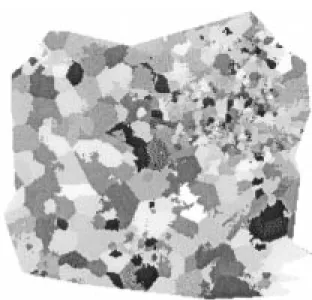
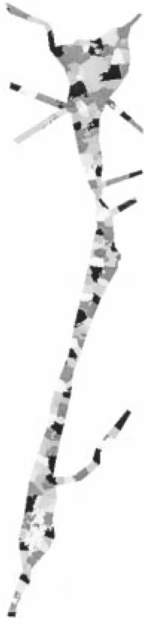
In all network designs, the number of iterations (trial net-works tested) needed to generate the final design lies between 5000 and 20 000 and requires a total computation time of no more than 48 h on a 400-MHz computer with 512 MB RAM running C++ code. Figs. 9–12 contain illustrative graphics
rep-Fig. 9. Example design for Town .
Fig. 10. Example design for Town .
resenting cell designs produced by the design process for the four problem instances.
VI. CONCLUSION
We have presented a framework based on simulated annealing for generating cellular network designs. Within the framework, several neighborhoods are used for specific aspects of the de-sign. The framework can be used to generate completely new networks or to augment preexisting networks (by adding new sites and amending the existing network or just by adding new sites and keeping the existing network unchanged). Results in-dicate that the problem is tractable and that the framework is capable of producing designs with very high area coverage and traffic capacity but at the expense of a high number of sites (rel-ative to the lower bound on the minimum necessary) and a large amount of interferers at each service test point. The effect of these interferers can be reduced by an efficient frequency plan; however, reducing the amount of interference would make the generation of such a plan much easier. Future work will inves-tigate 1) network interference metrics, which, if included in the design framework, will be sympathetic to producing an effec-tive frequency plan, and 2) a more effeceffec-tive implementation of the handover objective.
Fig. 11. Example design for Road .
ACKNOWLEDGMENT
The author is especially grateful to the members of the ARNO Project Consortium for many interesting discussions and advice; in particular, A. Caminada (France Telecom), P. Reininger (Nortel Networks), L. Floriani (France Telecom), O. Sarzeaud (ECTIA, France), A. Berny (ECTIA, France), J. Bendisch (GMD, Germany), J. Zimmermann (GMD, Ger-many), R. Hoens (GMD, GerGer-many), J.-K. Hao (Universite d’Anger’s, France) and M. Vasquez (EERIE, France).
REFERENCES
[1] S. J. Fortune, D. M. Gay, B. W. Kernighan, O. Landron, R. A. Valen-zuela, and M. H. Wright, “Wise design of indoor wireless systems,” IEEE Computat. Sci. Eng., vol. 2, no. 1, pp. 58–68, 1995.
[2] H. D. Sherali, C. M. Pendyala, and T. S. Rappaport, “Optimal location of transmitters for micro-cellular radio communication system design,” IEEE J. Select. Areas Commun., vol. 14, no. 4, pp. 662–673, 1996. [3] K. Tutschuka, N. Gerlich, and P. Tran-Gia, “An integrated cellular
net-work planning tool,” in Proc. 47th IEEE Vehicular Technology Conf., 1997, pp. 765–769.
[4] P. Calegarie, F. Guidec, P. Kuonen, B. Chamaret, S. Udeba, S. Jos-selin, and D. Wagner, “Radio network planning with combinatorial algorithms,” ACTS Mobile Commun., pp. 707–713, 1996.
Fig. 12. Example design for Road .
[5] J. McGeehan and H. Anderson, “Optimizing microcell base station lo-cations using simulated annealing techniques,” in Proc. 44th IEEE Ve-hicular Technology Conf., 1994, pp. 858–862.
[6] T. Fruhwirth, J. Molwitz, and P. Bisset, “Planning cordless business communication systems,” IEEE Expert Mag., pp. 662–673, 1996. [7] T. Lissajoux, V. Hilaire, A. Koukam, and A. Caminada, “Genetic
algo-rithms as prototyping tools for multi-agent systems: An application to the antenna setting problem,” in Lecture Notes in Computer Science, 1997, vol. 1437, pp. 17–28.
[8] A. Molina, G. Athanasiadou, and A. Nix, “The automatic location of base-stations for optimized cellular coverage: A new combinatorial ap-proach,” presented at the IEEE Vehicular Technology Conference, 1999. [9] L. Ibbetson and L. Lopes, “An automatic base site placement algorithm,”
presented at the IEEE Vehicular Technology Conf., 1997.
[10] G. Siqueira, E. Vasquez, R. Gomes, C. Sampaio, and M. Socorro, “Op-timization of base station antenna position based on propagation mea-surements on dense urban microcells,” presented at the IEEE Vehicular Technology Conf., 1997.
[11] F. Box, “A heuristic technique for assigning frequencies to mobile radio nets,” IEEE Trans. Veh. Technol., vol. VT-27, pp. 57–64, 1978. [12] D. Castelino, S. Hurley, and N. Stephens, “A tabu search algorithm for
frequency assignment,” Ann. Oper. Res., vol. 63, pp. 301–319, 1996. [13] P. Chan, M. Palaniswami, and D. Everitt, “Neural network-based
dy-namic channel assignment for cellular mobile communication systems,” IEEE Trans. Veh. Technol., vol. 43, no. 2, pp. 279–288, 1994. [14] J. Hao and R. Dörne, “Study of genetic search for the frequency
assign-ment problem,” in Lecture Notes in Computer Science, 1996, vol. 1063, pp. 333–344.
[15] I. Katzela and M. Naghshineh, “Channel assignment schemes for cellular mobile telecommunication systems: A comprehensive survey,” IEEE Personal Commun., pp. 11–31, 1996.
[16] R. Leese, “A unified approach to the assignment of radio channels on a regular hexagonal grid,” IEEE Trans. Veh. Technol., vol. 46, no. 4, pp. 968–980, 1997.
[17] D. Smith and S. Hurley, “Bounds for the frequency assignment problem,” Discrete Math., vol. 167/168, pp. 571–582, 1997.
[18] S. Hurley, D. Smith, and S. Thiel, “FASOFT: A system for discrete channel frequency assignment,” Radio Sci., vol. 32, pp. 1921–1939, 1997.
[19] S. Hurley and D. Smith, “Meta-heuristics and channel assignment,” in Methods and Algorithms for Channel Assignment, S. Hurley and R. Leese, Eds. Oxford, U.K.: Oxford Univ. Press, 2001. to appear. [20] P. Reininger and A. Caminada, “Model for GSM radio network
opti-mization,” presented at the 2nd ACM Int. Conf. Discrete Algorithms and Methods for Mobility, Dallas, TX, 1998.
[21] , “Connectivity management on mobile network design,” pre-sented at the 10th Conf. Eur. Consortium for Mathematics in Industry (ECMI-98), Goteborg, Sweden, 1998.
[22] J. Walfish and H. Bertoni, “A theoretical model of uhf propagation in urban environments,” IEEE Trans. Antennas Propagat., vol. AP-38, pp. 1788–1796, 1988.
[23] F. Ikegami, S. Yoshida, T. Takeuchi, and M. Umehira, “Propagation fac-tors controling mean field strength on urban streets,” IEEE Trans. An-tennas Propagat., vol. AP-32, pp. 822–829, 1984.
[24] M. Mouly and M.-B. Pautet, The GSM System for Mobile Communica-tions, 1992.
[25] E. Aarts and J. Lenstra, Eds., Local Search in Combinatorial Optimiza-tion. Chichester, U.K.: Wiley, 1997.
Stephen Hurley is a Reader in the Department of Computer Science and
Di-rector of the Centre of Mobile Communications, Cardiff University, Wales, U.K. Previously, he was with Ferranti Computer Systems, and the Numerical Algo-rithms Group, Oxford, U.K., designing efficient systolic array algoAlgo-rithms for recursive least squares problems arising in radar systems. He also was with the Safety and Engineering Science Division, United Kingdom Atomic Energy Au-thority, working on containment safety of nuclear power plants. He has pub-lished more than 80 scientific papers, mainly in the areas of fixed and mobile wireless network design, spectrum management, and combinatorial optimiza-tion. He was and is a Leader of several national and international projects in these areas.