Zurich Open Repository and Archive University of Zurich Main Library Strickhofstrasse 39 CH-8057 Zurich www.zora.uzh.ch Year: 2015
Improving investment decisions with simulated experience
Bradbury, Meike A S ; Hens, Thorsten ; Zeisberger, Stefan
Abstract: We apply a new and innovative approach to communicating risks associated with financial products that should support investors in making better investment decisions. In our experiments, participants are able to gain ”simulated experience” by random sampling of a previously described return distribution. We find that simulated experience considerably improves participants’ understanding of the underlying risk-return profile and prompts them to reconsider their investment decisions and to choose riskier financial products without regretting their higher risk-taking behavior afterwards. This method of experienced-based learning has high potential for being integrated into real-world applications and services.
DOI: https://doi.org/10.1093/rof/rfu021
Posted at the Zurich Open Repository and Archive, University of Zurich ZORA URL: https://doi.org/10.5167/uzh-109572
Journal Article Accepted Version
Originally published at:
Bradbury, Meike A S; Hens, Thorsten; Zeisberger, Stefan (2015). Improving investment decisions with simulated experience. Review of Finance, 19(3):1019-1052.
Improving investment decisions with simulated experience
This version: 2014-03-04Meike Bradburya, Thorsten Hensb and Stefan Zeisbergerc,*
a Department of Banking and Finance, University of Zurich, Switzerland bDepartment of Banking and Finance, University of Zurich, Switzerland,
Department of Finance, Norwegian School of Economics, Bergen, Norway
cDepartment of Banking and Finance, University of Zurich, Switzerland
*Corresponding author: [email protected], Tel.: +41 44 63 4 54 36, www.prospect-theory.com
Abstract
We apply a new and innovative approach to communicating risks associated with financial products that should support investors in making better investment decisions. In our experiments, participants are able to gain “simulated experience” by random sampling of a previously described return distribution. We find that simulated experience considerably improves participants’ understanding of the underlying risk-return profile and prompts them to reconsider their investment decisions and to choose riskier financial products without regretting their higher risk-taking behavior afterwards. This method of experienced-based learning has high potential for being integrated into real-world applications and services.
JEL classification: D81; G11
Keywords: Behavioral finance, simulated experience, experience sampling, investment decision, risk communication, financial advice
Acknowledgments
We are thankful to Brian Bloch, Peter Bossaerts, Colin Camerer, Thomas Langer, Chelsey Simmons, Noah Smith as well as to participants of the following conferences and seminars for their valuable comments and suggestions: Experimental Finance Conference (Innsbruck, Austria, 2011), Fourth Annual Meeting of the Academy of Behavioral Finance & Economics (New York City, USA, 2012), International Workshop Experimental Economics and Finance (Karlsruhe, Germany, 2012), Sino-Swiss Joint Workshop on Behavioral Finance and Quantitative Risk Management (Beijing, China, 2012), California Institute of Technology (CA, USA), University of Central Florida (FL, USA), Florida State University (FL, USA), University of Hannover (Germany), University of Innsbruck (Austria), University of Münster (Germany), Simon Fraser University (Canada), University of Sussex (UK), Stony Brook University (NY, USA) and University of Zurich (Switzerland). Many thanks also go to Reto Järmann, Dominik Schöni, and Alessandro Vagliardo for their assistance in running the experiments.
1. Introduction
In order to make appropriate investment decisions, it is essential for investors to know and understand the risks involved. However, the literature documents very low degrees of financial literacy among large parts of the population (see e.g. Lusardi and Michell, 2007) and investors lack a “feeling” for the trade-off between expected return and risk (Rieger, 2012). Even if risks are understood well it is important to find the right level of risk, given the possibly very consequential outcomes of investment decisions. Financial institutions should address these challenges and support investors in better understanding financial risks by communicating them more transparently, in particular for the layman. The common practice, however, is to use simple questionnaires to assess investors’ ability and willingness to take risks and to map these answers to investment propositions, rather than communicating risks directly. The link between questionnaire answers and recommended investments is not necessarily strong and often characterized by rules of thumb rather than any transparent theory (Nosic and Weber, 2010; Financial Service Authority, 2011; Pan and Statman, 2012). Also, the current way risk preferences are ascertained focuses on the “moment of decision” and ignores the moment outcomes are experienced, which can evoke emotions not likely foreseeable by investors (Kahneman, 2009).
Against this background, we challenge the current way risk preferences are assessed and mapped to investment advice. We suggest that rather than assessing risk preferences from scratch, financial advisors should communicate the opportunities and risks financial products hold in a way that guarantees investors an understanding of the risk-return trade-off. Our approach is based on important insights from the decision-making and behavioral finance literature, namely that risk preferences can differ considerably depending on whether people acquire information through description or (simulated) experience, referred to as the description-experience gap (Hertwig et al., 2004, for an overview see Rakow and Newell,
2010). Commonly, studies on the description-experience gap reduce the environmental complexity to a minimum and focus on very basic decision situations with two options and constant, at most binary, outcome possibilities. Kaufmann et al. (2013) were the first to transfer these insights to an investment decision context with real-world continuous outcome distributions. Using an online experiment, the authors find a greater average allocation towards a risky fund in the so-called “risk tool” condition (a combination of experience sampling and graphical illustration of the return distribution involved).
Believing in the importance of this research for financial decision-making, we conducted a series of experiments aimed at transferring these important insights to a close-to-real-world investment problem, involving the choice between financial products. In our experiments, subjects had to invest in financial products with different levels of capital protection twice. For the first decision, we informed the subjects verbally and in some cases supported by graphical illustration, about the relevant underlying return distribution of their investment. For the second decision, subjects additionally “experienced” the previously described distribution by random sampling of the underlying returns. Hence, subjects used an “investment simulator” to gain experience prior to actual investment decisions. Importantly, the simulated experience essentially repeated information already provided to the subjects, as they were informed about the return distribution and products prior to their first decision. However, the experience simulation aimed at presenting the trade-off between expected return and risk in a more comprehensible and, importantly, experiential way. Our main interest lies in whether and how simulated experience influences and changes risk-taking behavior for financial product choices on an individual level.
Our study extends previous research and differs in particular from Kaufmann et al. (2013) in three main ways. First, we apply a within-subject experimental design and can thus analyze whether subjects change their investment behavior due to gained experience. This is
important as Zeisberger et al. (2013) demonstrate that within-subject results in an investment context, in their specific case concerning myopic loss aversion, can differ substantially from what is expected from equivalent between-subject studies.1 A within-subject design also
solves many of the issues raised in the decision-making literature, such as information asymmetry between the description and experience conditions. Secondly, we particularly address the important issues of sampling bias. Random sampling as in the experience simulation can lead to “experienced distributions” that differ from the ones described if the amount sampled is small. This sampling error and the resulting information asymmetry might lead people to underestimate the occurrence of rare events, due to never sampled outcomes or treating always-sampled outcomes as less than certain (see Rakow and Newell, 2010 for an overview on this discussion). In contrast to Kaufmann et al. (2013) we ensure that everyone actively samples the same number of random returns and that this number of actively sampled return draws results in an unbiased sample of the underlying distribution. This is important, as the sampling bias has been shown to be a major driver for the description-experience gap (Hadar and Fox, 2009). Third, due to their popularity, we focus on financial products, capital-protected products in specific, rather than asset allocation decisions. The popularity of these products is usually explained by investors’ loss aversion or overestimation of loss probabilities (Döbeli and Vanini, 2010; Rieger, 2012). These products have gained increasing attention in the behavioral finance literature (see, for example, Breuer and Perst, 2007; Erner et al., 2013; Hens and Rieger, forthcoming). Given their asymmetric payoff structures, it is questionable whether previous findings can be transferred to these popular products.
1 To our knowledge ours is the only study besides Camilleri and Newell (2009) which analyzes the differences
Our results show a strong effect of simulated experience (SE) on product choice. Although we only offered a very limited number of financial products, a substantial proportion of our subjects changed their product choice from the first to the second decision. The product switches are systematic; subjects chose, on average, riskier products after they were able to gain experience. Importantly, these riskier decisions were, on average, not regretted in retrospect. Various control experiments show the robustness of our results and allow us to rule out alternative explanations for our findings. We further conclude that SE improves investors’ probability judgment and understanding of the risk-return trade-off. This is important as we do not want to impose greater risk-taking behavior on investors but rather aim at aligning investment decisions with actual risk preferences. Our results are robust with regard to the subjects’ socio-demographic characteristics. Even subjects who reported to be experienced in financial decisions change their risk taking after having gained SE.
2. Experimental design
2.1. General setup
The computer-based experiments were programmed using the software z-Tree (Fischbacher, 2007) and were carried out at the University of Zurich between 2011 and 2014. Overall, 535 students with different major study courses participated. The experiments took 65 minutes on average, including reading the instructions and the payout procedure.
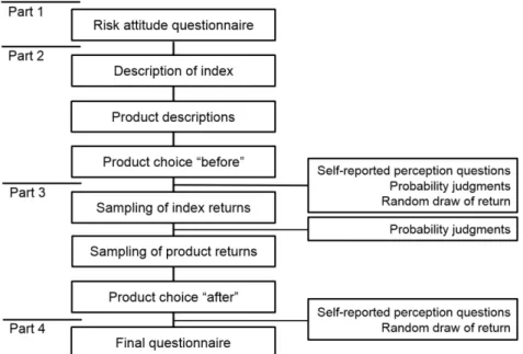
We conducted one base experiment and several control experiments with specific modifications to ensure the robustness of our results. The experiments followed a general design and consisted of four parts (see Figure 1). In the first part the subjects were asked to
answer questions concerning their general and financial risk attitude, followed by two binary lotteries regarding loss and risk aversion (see Appendix A).2
Figure 1: General experimental setup
This figure illustrates the overall sequence of the base experiment.
Part 2 started off with a verbal description of the underlying return index (details will be provided in Section 2.2, see Appendix B for an overview of the description-based decision part). The subjects were then presented with five capital protection products. The method of presentation aimed at guaranteeing the subjects’ full understanding of the investment choice to be made: We explained the functionality of the products using easy to understand wording and we provided a table with exemplary returns for the underlying index combined with the respective outcome of the product. Additionally, we showed a documented payoff diagram for each product. Each product was presented in the same way and on a separate screen (see
2 Self-assessed risk attitude questions are a common practice used for financial advice (Dohmen et al., 2009,
Nosic and Weber, 2010, Weber et al., 2012 and FinaMetrica for further specific example questions). Likewise, choice table procedures, similar to the methodology developed by Hault and Laury (2002), have gathered great attention in the literature on risk preference elicitation (see Weber and Johnson, 2008).
Appendix B 2 for details). After the presentation of the products, the subjects were asked to choose one of the five products they wanted to invest in (see Appendix B 3 for a screenshot). In Part 3 subjects gained SE. For that purpose, they drew a fixed number of random one-year returns of the index return distribution for the underlying index as well as for each product separately. For each index return the respective product return was depicted in a payoff diagram as introduced to the participants in Part 2 (see Appendix C for an example screenshot). After gaining SE, subjects had to make an investment decision in the same way as in Part 2, again followed by some questions.3
Part 4 concluded the experiments with a demographic questionnaire and some free text questions.
2.2. Underlying return index
The five financial products we offered to the subjects are based on the same underlying index, namely the S&P 500 index. To construct the index return distribution we calculated empirical one-year returns over 20 years (until 08/24/2011) using a one-day rolling time window, which resulted in 5,042 yearly (overlapping) returns. To avoid unintentional associations it was not revealed to the subjects that a specific index and time period was used (Weber et al., 2005). For the resulting distribution the average return amounts to 8.2% p.a. with a standard deviation of 18%, which was communicated to the subjects. As standard deviations have little intuitive meaning to most investors (Das et al., 2011) and because our empirical distribution is not perfectly (log-)normal, we additionally provided frequency information in the form of: “In [x] out of 100 cases the return was between …” with x=50,
3 Before the actual simulated experience part, subjects were presented with all five products side by side and
their respective payoff for three different (representative) index returns of the underlying index, namely –20%, +10%, and +40%. This eased the comparability between the products for different return scenarios.
90, and 95 (Appendix B 1 shows all relevant instructions as displayed to subjects on the computer screen).
2.3. Set of financial products
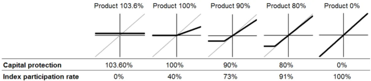
Subjects had to choose one of the five products to invest in. One product was risk-free and guaranteed subjects a sure payoff of 3.6% after one year. This represented the average yearly risk-free rate of US one-year Treasury bonds for our 20-year time period. The next three products all had a certain level of capital protection with respective index participation rates and the fifth product represented the underlying index itself, i.e. the market index without capital protection. Structures of the products were calculated using Black and Scholes (1973) arbitrage-free fair value framework.4 Figure 2 provides an overview of the products.
Throughout this paper the products will be named after their protection level: “90%” for example, indicates the product that protects 90% of the investment; “0%” thus represents the index product without any protection. To exclude order effects we used two different orders of product presentation in all experiments, keeping products in monotonic order of risk (we did not find a difference in product choice behavior between the two orders).
4 Of course, more sophisticated valuation frameworks exist. However, this should not be crucial to our analysis
since a different valuation would change the index participation rate both before and after simulated experience. Subjects also had full distributional information. A test experiment with log-normally distributed returns led to qualitatively the same results.
Figure 2: Product overview
Figure 2 illustrates the payoff profiles of the products for a one-year investment horizon (bold lines). The x -axis depicts the index return, the y-axis the respective product return.
2.4. Simulated experience
In the SE phase (Part 3), subjects sampled 30 times from the underlying return distribution, and, subsequently, 20 times for each of the five products. We decided to let each subject sample the random returns manually, and not to show automatically sampled returns, as Rakow et al. (2008) demonstrated that a process of active exploration can differ markedly from one of passive observation. Still, we wanted to keep the sampling quantity within a suitable range. Given these constraints, subjects sampled 130 independent, random returns from the same underlying distribution, which is sufficient to ensure that they sampled rare events such as an index return below -20%.5 By comparison, participants in Kaufmann et al.
(2013) were able to sample for as long as they wanted. On average, subjects sampled 14.5 times, which is likely to cause sampling biases for the active sampling part (after sampling, a computer simulation displayed another eight draws and then built up the entire return distribution with increasing speed). Importantly, our experimental design thus allows us to largely rule out sampling bias as a possible driver for the results.
5 Each subject was shown different random returns. By sampling 130 times, however, the sampled distributions
were relatively representative. Three out of four the sampled an index return below -20% between 8 and 16 times (of 130 draws), while the totally representative number would be 12 (9.4%). The high number of samples thus guaranteed a representative number of drawings even for relatively extreme returns.
2.5. Monetary incentives
To ensure appropriate incentives we provided real monetary rewards for each subject. A subject’s payoff was mainly determined by his or her product choice: Each subject was endowed with 10,000 ECU (“Experimental Currency Units”, equivalent to 20 Swiss Francs (CHF) or 25 USD at the time of the experiment) to invest in one of the five products. At the end of the experiment one of the two product choices (either from Part 2 or Part 3) was randomly selected for payoff. A single one-year return of the stock index was drawn randomly out of the described distribution and, depending on the chosen product, the subject’s payoff was determined. If, for example, for that random index return, the product’s return amounted to +10%, the payoff for the subject was (1+0.1)·10,000 ECU = 11,000 ECU or 22 CHF (27.50 USD).
The lottery-type risk preference questions in Part 1 were also incentivized: Subjects were endowed with 2,000 ECU, corresponding to 4 CHF (5 USD), for each of the two lottery questions. One of the two lottery questions was randomly determined and paid out in real money at the end of the experiment, following the Becker-De Groot-Marschak mechanism (Becker et al., 1964). Finally, subjects were paid a maximum of 4 CHF depending on the accuracy of their probability judgments.6 On average, each participant earned approx. 26
CHF (32.50 USD). The payment procedure was explained in the instructions (see Appendix D), which were read out aloud by the experimenter before the start of each part of the experiment. Additionally, the written instructions were handed out to each subject and could be consulted again throughout the experiment.
6 This amount was reduced linearly by the sum of absolute deviations of estimated probabilities from actual
probabilities. This amount was zero if this sum exceeded 120pp. Subjects were informed that their payment positively correlated to the overall accuracy of their estimates.
Regarding the experiment in general, we aimed at providing instructions that guarantee subjects’ full understanding of the experimental task. We tested this with a questionnaire at the end of the experiment. Subjects’ response to “Given the possible complexity of the experiment, how clear were the instructions?” (from 1 “not at all clear” to 6 “very clear”) was that 82% answered 5 or 6 while only 3% answered 1 or 2. The answers to an equivalent question on the usability of the software were: 93% in the upper vs. only 2% in the lower third. These responses provide evidence that our instructions and the software were appropriate.
3. Results
3.1. Investment decisions
In our base experiment 105 students participated, 54% of whom were female. The participants’ age ranged from 18 to 45 years with a mean age of 22.7 years. Nearly one quarter of the subjects reported to own or have already owned financial products.
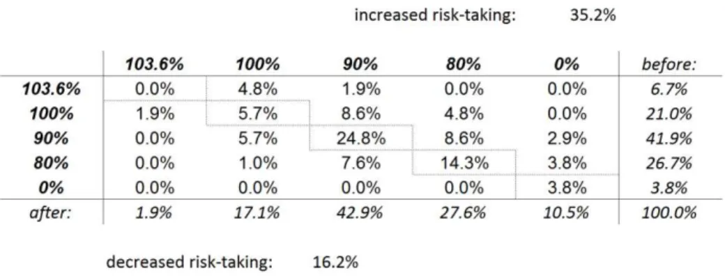
We find that SE leads to a significant reconsideration of investment decisions. After gaining experience 51.4% of subjects changed their product choice. Importantly, subjects chose, on average, significantly riskier products after SE: 35.2% increased risk taking while only 16.2% switched into a less risky product (paired two-sided Wilcoxon signed-rank test: p<0.01). Figure 3 presents a transition matrix of product switches.
Figure 3: Within-subject product switch matrix in the base experiment
This matrix shows the product choice percentages before simulated experience in the rows, and the percentages after simulated experience (SE) in the columns. In each cell one can read the percentage of
subjects, which switched from one product to another. The “4.8%” in the second row and fourth column, for example, indicate that 4.8% of all subjects chose the 100% capital protection product before SE and the 80% product after SE. The upper-right area indicates more risk taking after SE, the lower left area less risk taking.
We thus observe a higher risk taking even for a within-subject design and a product choice rather than an asset allocation decision. Additionally, our results demonstrate that the observed higher risk taking cannot be explained by sampling bias. To test for possible recency effects, i.e. whether decision-makers focus on the most recently sampled returns for making their decision, we measured the correlation between the sampled returns and product chosen. We do not find any significant relation for various different measures, including: all returns sampled; last 5, 10, or 20 returns sampled. We also do not find a systematic influence of the mean return drawn for different products on product choice at an individual level.
3.2. Feeling informed, confident and satisfied with investment decision
An important question is whether the riskier decisions based on SE are “right” or “better” for each individual. It is generally difficult to answer this question as one can only observe revealed preferences and it is hard to define a rational benchmark. Given this challenge, our approach is rather to measure whether the underlying risks of an investment are well understood and if investors are aware of the possible financial consequences they are about to take. In this regard investors will be more likely to anticipate their reaction to possible outcomes correctly and are able to incorporate their emotional responsiveness into their
decision-making process. We analyze subjects’ understanding of the risk-return relationship in two ways: subjectively, via self-reported perception questions, and objectively, via specific probability judgments.
Before and after SE, we asked subjects how well informed they feel about the product choice task they are about to make using a 6-point Likert scale (1 = not at all, 6 = very). We further asked them to state their confidence in having chosen the right level of capital protection. After they were shown the payment-relevant random return draw (and their actual return depending on their chosen product) we also asked about their satisfaction with their product choice. We find that subjects feel significantly better informed after SE (4.59 after vs. 4.24 before, two-sided Wilcoxon paired test p<0.01). They also feel more confident in having chosen the right level of capital protection after SE (4.39 vs. 4.17, p=0.08). At the same time we do not find a significant change in levels of satisfaction between the two conditions, although they, on average, take significantly higher financial risks and hence are potentially exposed to greater downturns of returns after SE (4.08 vs. 4.23, p=0.41).
3.3. Probability judgments
To obtain an objective measure of subjects’ decision-making ability and the stock index return distribution, we requested subjects to estimate the following: the expected return, the probability of a loss (measured from the initial monetary endowment), the probability of a loss (and gain) larger than 10% and 20%. Subjects were asked to estimate these probabilities twice, first directly after being presented with the underlying return distribution in a verbal manner, and secondly after having gained SE of the index.
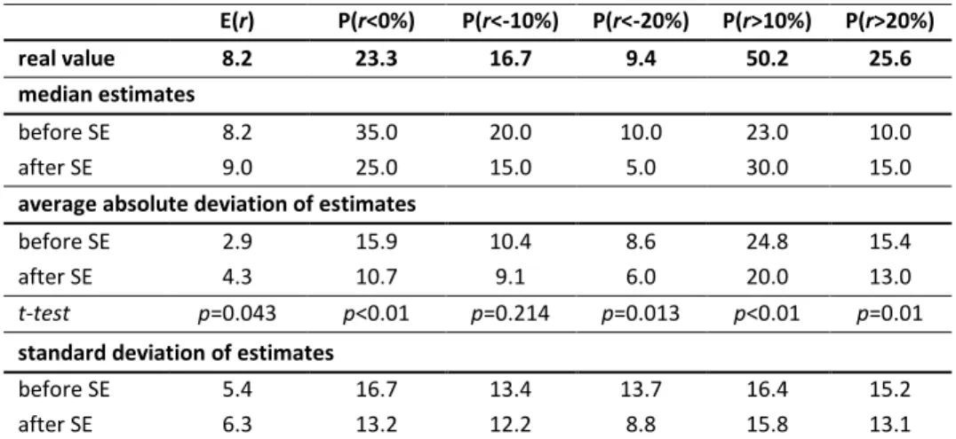
For the judgments made directly after the description part we observe that subjects overestimate probabilities of a loss and underestimate probabilities of a gain, on average (see Table 1). All mean estimates improve through SE (apart from the question on the expected
return, which can be explained by the fact that this return was stated explicitly in the description part). As a result, loss probabilities are no longer overestimated after SE. Estimates of the gain probability also significantly improve, although they are still underestimated on average. Mean absolute deviations per subject and standard deviation among all subjects also decrease significantly. We conclude that SE reduces biased expectations and thus improves investors’ understanding of the risk-return trade-off. Note that the probability judgments after SE were intentionally conducted after the sampling of the index—and thus before SE of the products—in order to avoid product return distributions being mixed up with that of the index. Hence, probability estimates after SE are based on the observation of only 30 random returns leading to higher sampling error.
Table 1: Real and estimated characteristics of the index return distribution
E(r) P(r<0%) P(r<-10%) P(r<-20%) P(r>10%) P(r>20%) real value 8.2 23.3 16.7 9.4 50.2 25.6 median estimates before SE 8.2 35.0 20.0 10.0 23.0 10.0 after SE 9.0 25.0 15.0 5.0 30.0 15.0
average absolute deviation of estimates before SE 2.9 15.9 10.4 8.6 24.8 15.4 after SE 4.3 10.7 9.1 6.0 20.0 13.0
t-test p=0.043 p<0.01 p=0.214 p=0.013 p<0.01 p=0.01
standard deviation of estimates before SE 5.4 16.7 13.4 13.7 16.4 15.2 after SE 6.3 13.2 12.2 8.8 15.8 13.1
This table shows real values and related subjects’ median estimates for different return thresholds of the underlying index return distribution (P(r…)) in the upper panel. In the middle panel average absolute deviations per subject are shown and in the lower panel subsequent standard deviations of estimates over all subjects are presented. To calculate the p-values of the two-sided (paired) t-tests we use absolute deviations from estimated to real values to avoid opposite signs canceling each other out. For the same reason we show absolute rather than signed deviations in the table.
Our results confirm findings from the decision-making literature on the description-experience gap to cause closer alignments between estimated and objective probabilities through SE (see Hau et al., 2008) and show that they are transferable to finance. They also confirm the findings of Kaufmann et al. (2013) who used predefined intervals for the judgments about expected return and open questions for judgments about a loss and a high
gain. Concerning our question from the beginning of this section, namely whether SE leads to “better” decisions, the presented findings clearly point towards improvements, since biased expectations are significantly reduced.
4. Discussion and robustness of results
We conducted several control experiments, beginning with small and then extending those to more extreme variations (see Appendix E for an overview of all experiments). The control experiments aim to exclude alternative explanations that might drive our results and at increasing the universal validity of our main findings.
4.1. Experimenter demand effect
The first control experiment (1) addresses a possible experimenter demand effect since we advised subjects in the instructions of the SE part, for example, to “take the opportunity to improve your understanding of the return distribution.” To exclude the possibility that participants’ answers are biased due to this statement we repeated the experiment and excluded critical parts in the instructions; all other parts remained exactly the same. In total, 63 subjects took part in this replication.
All qualitative results of the base experiment can be confirmed and some results are even stronger. We observe that 38.1% of participants increase their risk taking after SE, only 7.9% decrease it (p<0.01). Subjects also feel significantly better informed (4.87 vs. 4.30, p<0.001) and are significantly more confident of having made the right product choice (4.51 vs. 4.19,
p=0.04). Similar to the base experiment the increased risk taking is not regretted afterwards: participants’ satisfaction stayed at the same level (4.30 vs. 4.29, p=0.95). Also, the
probability estimates for the index return distribution improved considerably (p≤0.03 for all
five probability questions).7
4.2. Order effects
The following robustness check relates to the order of the description and experience parts, given our within-subject design. Greater risk taking after SE could simply be the result of the fact that subjects first made a product choice based on description and subsequently based on SE. Or in other words: Greater risk taking after SE could be influenced by the fact that after explaining the same problem twice, but in different ways, subjects understood it better and hence took more risk the second time around. To investigate this possibility, we ran control experiment (2) in which subjects first went through the SE phase—without having been informed about the index return distribution verbally—and subsequently obtained the descriptive information on the index. An additional 48 subjects with very similar demographic characteristics to those the base experiment participated.
Generally speaking, this robustness check provides evidence that our main findings are not driven by undesired order effects. The product switches are no longer systematic: 18.8% choose a riskier product while 25.0% switch into a less risky product for the second decision (p=0.35). We also find no significant difference in chosen risk levels after SE between the base experiment and this control experiment (between-subject Wilcoxon test: p=0.97). Furthermore, we neither find an increase in feeling informed nor in feeling confident by receiving the descriptive information in addition to and after SE. Subjects even stated significantly lower levels of feeling informed (4.10 vs. 4.56, p<0.01) and confidence (4.06 vs.
7 We continue without reporting probability estimates on the expected return, which did not improve based on
SE throughout all control experiments, due to the fact that this probability was stated explicitly in the description part. An overview of all the results in detail and for all experiments can be provided by the authors upon request.
4.38, p=0.02) after receiving the descriptive information. This result suggests that SE improves an investor’s comprehension whether or not he or she has received other information previously. As in our base experiment we do not find a significant difference in satisfaction for the product choices between the two conditions (4.56 vs. 4.31, p=0.72). We conclude that it is SE that drives our findings and not the order of the conditions (description versus SE first).
4.3. Return realization effects
A further possible check we felt necessary to analyze, addresses the payment-relevant return draw. In our base experiment the random, payment-relevant return was drawn directly after each of the two product choices—which was done intentionally to measure satisfaction with the decision directly after the return draw and before SE. Consequently, subjects received feedback concerning their possible experimental payment before making the second product choice. This might have caused an order-related effect due to the house money and/or a break-even effect (Thaler and Johnson, 1990).8 Generally, we countervailed these possible
effects by making only one random draw payment-relevant (either the one in Part 2 or the one in Part 3), which we clearly communicated to subjects (see also Azrieli et al., 2012). However, to rule out any possibility of order-related effects concerning the payment-relevant return draw we conducted a further control experiment (3) in which both payment-relevant return draws followed after the second investment decision (end of Part 3). Overall, 71 subjects participated. The results of this control experiment confirm the findings of our base experiment. We find even stronger changes in risk taking compared to the base experiment after SE, with 25.4% of subjects choosing a riskier and only 8.5% choosing a less risky product (p=0.025). The overall switching rate is lower, with 33.9% compared to 51.4% in the
8 The house money effect would predict more risk seeking after gains, the break-even effect would also predict
base experiment. Furthermore, feeling informed increases substantially (4.51 vs. 4.03,
p<0.01) and so do the probability estimates after SE improve (p<0.03 for all probability estimates). Again, levels of satisfaction do not differ markedly between the two conditions, just as observed in our base experiment. Subjects’ confidence in having made the right investment decision increases from 4.11 to 4.23; however, this change is not significant (p=0.38).
To rule out any combined order effects, we conducted control experiment (4) applying both changes of control experiments 2 and 3 simultaneously (SE before description and both payment-relevant return draws only after Part 3). All other details of the experimental design remained unchanged. Overall, 69 subjects participated. The results confirm our findings presented above. In particular, we neither observe any significant directional switching behavior in product choices (15.9% of participants increase and 18.8% decrease risk taking,
p=0.72) nor do we measure a significant change in feeling informed, confident or satisfied with the investment decision (all p>0.9). The still relatively high switch rate of 34.7% gives an indication that the descriptive index return information that was presented after the SE was not simply ignored, as found in Lejarraga and Gonzalez (2011).
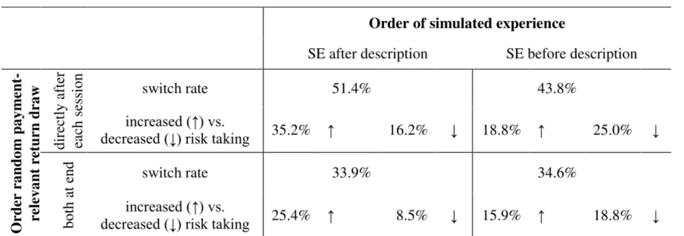
Table 2 provides an overview of product choices for all experiments mentioned so far. We clearly observe that SE leads to increased risk taking. Importantly, this effect is not reversed when changing the order of treatments (description vs. SE). We also observe switching rates to be lower if there is no intermediate payment-relevant return draws. We assume that the payment-relevant returns influence subjects more than non-payment-relevant SE draws.
Table 2: Overview of subjects’ product switching behavior for all experiments
Order of simulated experience
SE after description SE before description
O rder ra nd o m pa y ment -re lev a nt re turn dra w d ir ec tly af ter ea ch s ess io n switch rate 51.4% 43.8% increased (↑) vs.
decreased (↓) risk taking 35.2% ↑ 16.2% ↓ 18.8% ↑ 25.0% ↓
b o th at en d switch rate 33.9% 34.6% increased (↑) vs.
decreased (↓) risk taking 25.4% ↑ 8.5% ↓ 15.9% ↑ 18.8% ↓
This table reports switching rates and percentages of subjects increasing and decreasing the chosen risk level from the first to the second decision for all experiments. The base experiment is shown in the upper-left panel of the four panels.
4.4. Information asymmetry
The following robustness check addresses possible information asymmetry between the description and SE parts. SE might provide more information about the index return distribution than the description because we used an empirical return distribution for the index that is not perfectly (log-)normal. We therefore ran a further control experiment (5), in which we showed subjects (n=80) the stock index return distribution using a detailed bar chart (see Appendix F) with a reading example in addition to the verbal explanation.9
Consequently, subjects were provided with full information about the distribution in the description part. Subjects spent a median time of 55 seconds on the screen showing the descriptive return information and they were told to pay attention to this information.
This additional information did not affect subjects’ product choice behavior. We observe a significant increase in risk taking after SE: 37.5% of subjects increased their risk taking while
9 Additionally, we made very minor changes to the text to eliminate any possibility of leftover experimenter
demand effects, based on control experiment 1. In particular, we deleted the sentences “The sampling of random returns serves to give you a feeling for the return distribution and has no payment relevance” and “Our goal is to
find a customer-friendly form of investment advice. With the results we hope to achieve an improvement for the
financial industry.” and later in Part 3 we changed “After gaining experience” in “After that.” We also deleted
only 11.3% decreased it after SE (p<0.001). The more transparent communication of the stock index return distribution, however, seems to influence subjects’ self-evaluation of feeling informed. Average feeling informed amounts to 4.41 after and 4.39 before SE, so that we do not observe a significant improvement anymore. Similarly, our “feeling convinced” measure does not change (4.06 after vs. 4.25 before, p=0.15). As before, there is also no significant change in satisfaction levels after having received the payment-relevant return draw (4.18 vs. 4.00, p=0.51). These results are to some extent in contrast to Kaufmann et al. (2013) as they find differences in these measures. However, the authors used a between-subject design and a probability density function. We believe that the bar chart is easier to read and understand compared to a probability density function. Therefore, Kaufmann et al. (2013) still find subjects feel better informed after experience sampling. While self-reported perception measures did not improve in our new setting, we still find a significant improvement in probability judgments. All five average probability estimates were significantly closer to the real values after SE.
In a test experiment with a slightly different design we used a log-normal return distribution for the index. Although we do not want to overplay our findings of this test experiment due to some differences in the setup and products, the qualitative results are the same. In particular, SE leads to higher risk taking, i.e. lower levels of capital protection. We also confirm an improvement in probability estimates. Generally speaking, our findings seem to be independent of the distributional form of the index returns.
4.5. Experiment complexity
Due to the relatively high complexity of our experiment compared to typical judgment and decision-making research, subjects might have been confused in early parts of the experiment and hence might have been more risk averse for the first product choice. We analyzed our results again and excluded all subjects that did not state that the instructions were clear. In
particular, we excluded subjects that did not respond 5 or 6 on the scale of the instruction clarity question (see Section 2.5). Generally speaking, there are hardly any quantitative changes to our results if we exclude subjects who were not satisfied with the instructions. Consequently, our results seem not to be driven by confused subjects.
As a further robustness check we ran another control experiment (6) in which we greatly reduced the experiment’s complexity. More precisely, we made the following changes to control experiment (5), outlined in Section 4.4. First, we excluded Part 1, as the quantitative risk preference questions might have led to confusion with later return distributions. Second, we made the product description screenshots less busy by excluding the table. To enhance subjects’ understanding of the products we included a product overview table, comparing each product side by side for three different return scenarios of the index return and product returns respectively, right after the product descriptions. Third, we also implemented a test on subjects’ product understanding. Subjects could only continue with the experiment if they answered all four questions correctly. Subjects again were presented with the index return distribution and a commented bar chart.10
Despite these simplifications in the experimental setup and a higher transparency, we find the same results as in control experiment 5, which also included the bar chart. Subjects (n=99) choose, on average, riskier products: 40.4% increased vs. 15.2% decreased risk taking (p<0.001). Self-reported values for feeling informed, confident and satisfied do not change significantly: informed (4.62 after SE vs. 4.55 before, p=0.51), confident (4.18 vs 4.27,
p=0.44), satisfied (4.70 vs. 4.42, p=0.16). Importantly, all probability judgments improve significantly, as in all previous experiments. Hence, our results hold true even for a setting
10 Instructions were adapted to the new setup of control experiment 6, i.e. omitting parts no longer required, and
with reduced complexity and higher transparency. We conclude that experiment complexity is very unlikely to be driving our general findings.11
4.6. Generalizability of results
A deeper analysis of our data in the base experiment reveals that the switching behavior is a relatively stable and general phenomenon. It is not driven by personal characteristics such as investment experience or gender (and we intentionally recruited our subjects from all major study courses). We measure experience by self-reported ownership of financial or structured products and/or in-depth study of financial and structured products. Male, female, experienced, and inexperienced subjects alike take higher risks with SE (paired Wilcoxon tests for the base experiment: men: p=0.015, women: p=0.042, experienced: p<0.01, inexperienced: p=0.106).
5. Investment decision predictability
Given the motivation of our paper, i.e. to challenge the current practice of financial institutions on assessing customers’ risk attitudes and mapping them to investment propositions, an analysis of the link between self-reported risk preferences and investment decision is important and could allow fruitful insights. We are particularly interested in the question of how this link differs before and after SE. For this reason, subjects in our experiments had to answer a series of questions concerning risk attitudes in Part 1 of the experiment. The questions also encompassed two quantitative measures in the form of paid lottery tasks, one referring to loss aversion and the other to risk aversion (i.e. curvature of value function). For the lottery questions we used a decision matrix in a price list style, aimed
11 We further asked the question on the clarity of instructions immediately after the first product choice. On the
6-point Likert scale 85.9% of subjects answered with high values of 5 or 6, i.e. confuting the assumption that the instructions might have been unclear.
at eliciting subjects’ certainty equivalents, similar to Holt and Laury (2002), which thus forms a quantitative measure for loss and risk aversion (see Appendix A; for an overview of quantitative risk preference elicitation procedures see Wakker and Deneffe, 1996).
For the decisions before SE we observe the quantitative loss aversion measure to have a highly significant predictive power, see Table 3, Model (1). This holds true even when including quantitative risk aversion, qualitative self-reported general risk and financial risk aversion as control variables as in Model (2).
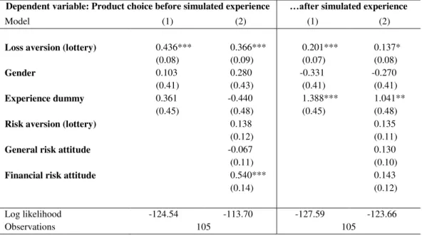
Table 3: Product choice predictability before and after simulated experience
Dependent variable: Product choice before simulated experience …after simulated experience
Model (1) (2) (1) (2)
Loss aversion (lottery) 0.436*** 0.366*** 0.201*** 0.137*
(0.08) (0.09) (0.07) (0.08)
Gender 0.103 0.280 -0.331 -0.270
(0.41) (0.43) (0.41) (0.41)
Experience dummy 0.361 -0.440 1.388*** 1.041**
(0.45) (0.48) (0.45) (0.48)
Risk aversion (lottery) 0.138 0.135
(0.12) (0.11)
General risk attitude -0.067 0.130
(0.11) (0.10)
Financial risk attitude 0.540*** 0.143
(0.14) (0.12)
Log likelihood -124.54 -113.70 -127.59 -123.66
Observations 105 105
This table reports results of the ordered logit regressions with the product choice before (second and third column) and after (last two columns) simulated experience as the dependent variable, coded 1 to 5 according to their riskiness for 103.6%, 100%, 90%, 80% and 0% capital protection. Six-point Likert scale answers on qualitative risk-attitude questions are treated as ordinal independent variables. Standard errors are in brackets. * indicates significance at the 10% level, ** 5% level, and *** 1% level. We checked the “tolerance” and
“variance inflation factor (VIF)” values for multicollinearity, which are all statistically acceptable (the maximum VIF out of the explanatory variables is 1.8).
For the decisions after SE the results change. The qualitative loss aversion coefficient becomes considerably smaller in Model (1)—although it remains significant. In Model (2) the coefficient only remains marginally significant. Similarly, the qualitative financial risk aversion question loses its predictive power after SE. Investment experience, on the contrary,
becomes a predictor for risk-taking behavior; more experience implies a riskier product choice.
In conclusion, it becomes relatively difficult in our experiment to predict product choices based on self-reported risk attitude or lottery questions once subjects were able to gain investment experience. These findings further underpin the difficulty of defining individual risk attitudes and preferences based on questionnaires, in particular if investors’ understanding of financial products is improved based on SE.
6. Conclusions and final remarks
In this paper we challenge the status quo of financial advice and apply a novel approach to communicate risks associated with financial products. Our approach is inspired by previous research that demonstrates a strong difference between decisions from description and decisions from experience (see, in particular, Kaufmann et al., 2013). Rather than describing an investment problem or asking investors about their willingness to take risks, we find evidence that it is advantageous for investors to directly experience the consequences of their financial decisions prior to making an investment, i.e. to gain SE. This is of particular importance as many investors lack basic knowledge about financial products and about how much risk is involved or because they have biased return expectations. Such products are also known to exploit investment biases (Rieger, 2012).
Our experimental results give evidence that investment decisions can be considerably improved by letting potential investors gain simulated experience. When making experience-based investment decisions investors are likely to switch to riskier products compared to investment decisions based purely on description. Importantly, we find this greater risk taking to be accompanied by a better understanding of the underlying risk-return profile, i.e. a lower mis-estimation of the associated return probabilities. After SE, loss probabilities are
less overestimated, gain probabilities less underestimated, likely explaining higher risk-taking. In addition, subjects do not show greater regret or dissatisfaction with the returns achieved by the riskier decisions. These findings suggest that SE prepares investors to better anticipate potential losses, which, we believe, is a considerable improvement to the status quo. We do not find effects to be smaller for subjects that already possess financial products and/or have experience with financial markets.
Our study extends previous research in several important aspects and thus offers important insights for research as well as business practice. From a scientific viewpoint, our within-subject experimental design allows us to confirm the previous findings of Kaufmann et al., 2013 but on an individual level and for a close-to-real-world setting, involving the choice between risky financial products and an underlying empirical return distribution. Contrary to many other studies on the description-experience gap, we are able to rule out several alternative explanations for increased risk-taking behavior after SE. In particular, our results cannot be explained by sampling bias or information asymmetry, nor do we find any evidence for recency effects. From a business practice perspective, our research provides arguments for including methods that allow customers to gain SE in financial advisory processes. By enabling investors to better calibrate expectations and possible outcomes they will less likely regret their product choices even if the realized returns are not favorable. We know of a large European online bank which is currently implementing a tool similar to the one we presented here. Furthermore, we contribute to the discussion on whether and how risk attitude measures, as currently used in banking practice, correspond with actual investment behavior. While there is predictive power of some typically used risk attitude questions for investment decisions based on description, this predictive power is considerably lower for decisions based on experience. Arguing that experience-based decisions are superior, we thus challenge the current way risk preferences are assessed and interpreted.
APPENDIX A: Risk Attitude Questions in Part 1
A 1 Lottery choices for loss and risk aversion
risky asset choice risk-free
asset 50% probability 50% probability I prefer the risky asset I prefer the risk-free asset 100% probability 10 % 0 % 〇 〇 0 % 10 % -1 % 〇 〇 0 % 10 % -2 % 〇 〇 0 % 10 % -3 % 〇 〇 0 % 10 % -4 % 〇 〇 0 % 10 % -5 % 〇 〇 0 % 10 % -6 % 〇 〇 0 % 10 % -7 % 〇 〇 0 % 10 % -8 % 〇 〇 0 % 10 % -9 % 〇 〇 0 % 10 % -10 % 〇 〇 0 %
risky asset choice risk-free
asset 50% probability 50% probability I prefer the risky asset I prefer the risk-free asset 100% probability 10 % 0 % 〇 〇 0 % 10 % 0 % 〇 〇 1 % 10 % 0 % 〇 〇 2 % 10 % 0 % 〇 〇 3 % 10 % 0 % 〇 〇 4 % 10 % 0 % 〇 〇 5 % 10 % 0 % 〇 〇 6 % 10 % 0 % 〇 〇 7 % 10 % 0 % 〇 〇 8 % 10 % 0 % 〇 〇 9 % 10 % 0 % 〇 〇 10 %
Design of the two price list-style lotteries as they appeared on the computer screen. For each line the subjects were required to state their preference between the risky and the risk-free asset. If a subject changed from preferring the risky asset to preferring the risk-free asset and switched back again, a message appeared on the computer screen that informed them that they had switched between the two options more than once and that they were requested to reconsider their decision.
Numerical loss and risk aversion is determined by the midpoint of switching from the risky to the safe option. A reference point of 0% is assumed.
A 2 Risk attitude questions General risk
attitude
Are you generally willing to take risks or do you try to avoid them? Strongly avoid risks o o o o o o o o o o willing to take risks Financial risk
attitude
How would you classify your willingness to take financial risks? Strongly avoid risks o o o o o o o o o o willing to take risks Willingness
financial risks
Which of the following statements best describes your willingness to take financial risks?
o Do not accept financial risks whatsoever
o Accept minor risks in anticipation of minor returns o Accept average risks in anticipation of average returns
o Accept above average risks in anticipation of above average returns o Accept considerable risks in anticipation of considerable returns
A 3 Emotionally attached risk attitude questions
Losses vs. gains In financial decisions, both gains and losses are possible. To what extent do possible losses compared to possible gains influence you?
Protection against losses is the most important to me o o o o o o participation in high returns is the most important to me
Confidence How much confidence do you have in your ability to make good financial decisions?
No confidence in own ability o o o o o o high confidence in own ability Optimism Are you more an optimistic or pessimistic person?
Very pessimistic o o o o o o very optimistic Mood In what mood are you at the moment?
Very bad mood o o o o o o very good mood
Interest Do you enjoy conversations about money and financial investments? Not at all o o o o o o very much
Anxious Are you anxious about investing money or making financial decisions? Not at all o o o o o o very much
Worried Do you worry about the success of your financial decisions? Not at all o o o o o o very much
Intuition Do you think that investment decisions just depend on instincts in the end? Not at all o o o o o o very much
Scared Are you scared of making losses with financial decisions? Not at all o o o o o o very much
Delegate Would you prefer to delegate financial decisions? Not at all o o o o o o very much
A 4 Control variables
Experience 1, if subjects owned financial products before or if they have extensively studied financial and structured products, 0 otherwise.
APPENDIX B: Part 2 (description-based decision)
B 1 Instructions on computer screen:
In the following you have to choose one out of five financial products. The products returns depend (each in a different way) on a risky stock index, which tracks the price development of stocks. Over the last 20 years this price development was characterized by fluctuations. In this time period the stock index possessed
an annual return of 8.2%
and a return standard deviation of 18%.
In 50 of 100 cases the annual return was between +1.3% and +20.2%. In 90 of 100 cases the annual return was between –25.4% and +34.2%. In 95 of 100 cases the annual return was between –36.3% and +39.1%.
Out of this 20-year period with the above given characteristics we will draw one 1-year-return randomly which is then relevant for your payment. Your 1-year-return is determined by this random return and the financial product you have chosen.
B 2 Screenshot Product Description Part 2
English translation:
[Title:] Product B: With this product there are no losses possible, i.e. after one year you receive at least 10,000 ECU. If the return of the index after one year is positive, your return is 40% of the index return.
[Table:] Hypothetical returns of the stock index and payoff for product B after one year: / Return Stock Index / Return Product
[Diagram caption:] This figure presents the product’s payoff after one year depending on the stock index. On the x-axis the return of the stock index is shown and on the y-axis the respective return of the product.
[Product descriptions on computer screen (each product was presented on a separate screen):]
Product Description
103.6%: The return of this product is a sure return of 3.6% after one year.
100%: With this product there are no losses possible, i.e. after one year you receive at least 10,000 ECU. If the return of the index after one year is positive, your return is 40% of the index return.
90%: With this product your loss is limited to a maximum of 10%, i.e. after one year you receive at least 9,000 ECU. If the stock index return is higher than −13.7%, your return is 73% of the stock index return exceeding this value.
80%: With this product your loss is limited to a maximum of 20%, i.e. after one year you receive at least 8,000 ECU. If the stock index return is higher than −22.0%, your return is 91% of the stock index return exceeding this value.
0% (index): The return of this product equals the return of the stock index after one year.
B 3 Screenshot Product Choice (Parts 2 and 3)
English translation:
Bezahlungsrelevante Frage = Payment relevant question
[Title:] Decide now in which of the five products you want to invest your 10’000 ECU.
Rendite =return / Aktienindex = stock index / Produkt = product / Produktwahl = product choice / Weiter = next.
APPENDIX C: Screenshot of simulated experience part in experiment
This figure shows a screenshot for the simulated experience section, here of the product with 90% capital protection and an upside participation rate of 75%. The last sampled return is 26.34% for the index, which results in a product return of 19.22%.
English translation:
Produkt C = product C / Rendite Produkt = product return / Rendite Index = index return / Ziehung = draw.
APPENDIX D: Paper instructions (translated from German)
D 1 Instructions (were handed out in paper and read aloud)
[Note: The instructions for the different parts were distributed and read aloud immediately before the beginning of the respective part, i.e. for Parts 2, 3 and 4 after all subjects had finished the previous part, for Part 1 directly after the overall instructions]
D 2 Base experiment [control experiment 5 adaptations]
Research study investment decisions Dear participants,
[Base experiment: Thank you very much for taking part in this study. Our goal is to find ways for a customer-friendly form of investment advice. With the results we hope to contribute to an improvement of the financial industry. Generally speaking, you will have to make some investment decisions and answer accompanying questions during this research study. The study consists of four parts.]
[Control experiment 5: Thank you very much for taking part in this study. Generally speaking, you will have to make some investment decisions and answer accompanying questions during this research study. The study consists of four parts.]
Your payment:
All payment-relevant questions are clearly marked in red. For these questions you will be given an investment capital in ECU (“Experimental Currency Units”). Depending on your investment decisions, you can realize profits but also suffer losses. You are paid at the end of the experiment in real Swiss francs. The exchange rate is 1:500, hence 10,000 ECU correspond to 20 Swiss Francs. Further information will be provided in the respective parts of this study.
For each part of this study precise instructions will be provided. Please read these instructions carefully. If you have questions or feel uncertain about what to do, please raise your arm and the experimenter will help you as quickly as possible. It is very important to us that you understand the content of this study correctly, and that you answer according to your true preferences. Also, please bear in mind that your payment is largely determined by your decisions.
Throughout the study communication with other participants is not allowed and the use of personal belongings such as cell phones or writing materials is also forbidden. Please use only those functions on the computer that are intended for the study. After each part you will have to wait until each participant has finished that part. The duration of the study is approx. one hour.
In the upper-right corner of this paper you will find a lab and computer number. Please take a seat at the respective computer.
Thank you very much in advance for your participation!
In the following first section we ask you to answer a few questions concerning your decision behavior. Afterwards you are kindly requested to decide between different financial investments. Our aim is to get to know your personal valuation, views and penchants for financial investments. Naturally there are no “wrong” answers; your answers should solely depend on your preferences.
Your payment:
For the payment-relevant questions you will have to decide multiple times between a risky and a risk-free asset. Your investment decisions can increase your investment capital for this part (2,000 ECU) but they can also decrease it. To determine your payment for this part, the computer will randomly choose one of your investment decisions:
If you chose the risk-free asset for this decision, you will receive the respective gain.
If you chose the risky asset, one of two scenarios is determined at random according to the stated probabilities. A resulting gain would be added to your investment capital, a loss would be deducted from it.
Part 2 [Base experiment: Investment decision]
In the following second part you will be asked to choose one of five products in which to invest.
The returns of the products depend on the return of a stock index. The stock index tracks the overall performance of stocks.
The return of the stock index is determined randomly. For this purpose, we will randomly pick an actually existing one-year period out of the last 20 years (a return the stock index has actually realized over the last 20 years). What returns are possible (the “return distribution”) are presented at the beginning.
Please take a careful look at the description of the stock index since it is important for your product choice!
[Control experiment 5:
The product return depends on the return of a stock index.
The stock index tracks the overall performance of stocks. As the overall
performance of stocks contains risk, there is a variety of different possible stock index returns. The probabilities of the different possible returns (i.e. the “return
distribution”) will be shown to you right at the beginning.
Please take a careful look at the description of the stock index since it is important for your product choice!]
For each product we will provide a description including a payoff diagram. The payoff diagram shows you how the stock index return is transformed into a product return and refers to a one-year time horizon in each case. The return of the stock index is depicted on the x -axis and the respective return of the product is depicted on the y-axis.
After the product description you will have to decide which of the five products you are going to invest in, and you have to answer a few additional questions.