Monetary consequences of alternative fiscal policy rules

BANK OF FINLAND

DISCUSSION PAPERS

20

•

2004

Jukka Railavo

Research Department

13.10.2004

Monetary consequences of

alternative fiscal policy rules

Suomen Pankin keskustelualoitteita Finlands Banks diskussionsunderlag

Suomen Pankki Bank of Finland P.O.Box 160 FIN-00101 HELSINKI Finland + 358 10 8311 http://www.bof.fi

BANK OF FINLAND

DISCUSSION PAPERS

20 • 2004

Jukka Railavo*

Research Department

13.10.2004

Monetary consequences of

alternative fiscal policy rules

The views expressed are those of the author and do not necessarily reflect the views of the Bank of Finland.

* E-mail: [email protected], Tel. 010 831 2932.

I am grateful to Juha Tarkka and Jouko Vilmunen for encouraging and helpful comments. Also the comments from Jarmo Kontulainen, Mikko Puhakka, Tuomas Takalo, Matti Virén and the participants of the Bank of Finland workshop on modelling monetary policy are gratefully acknowledged.

Suomen Pankin keskustelualoitteita Finlands Banks diskussionsunderlag

http://www.bof.fi ISBN 952-462-158-4 ISSN 0785-3572 (print) ISBN 952-462-159-2 ISSN 1456-6184 (online) Multiprint Oy Helsinki 2004

Monetary consequences of alternative fiscal policy

rules

Bank of Finland Discussion Papers 20/2004

Jukka Railavo

Research Department

Abstract

In this paper we analyse the monetary impact of alternative fiscal policy rules using the debt and deficit, both mentioned as measures of fiscal policy performance in the Stability and Growth Pact (SGP). We use a New Keynesian model, with endogenous labour supply, distortionary taxation and no private capital. The economy is hit by two fundamental shocks: demand and supply shocks, which are orthogonal to each other. Monetary policy is conducted by an independent central bank that will optimise. Under discretionary monetary policy the size of the inflation bias depends on the fiscal policy regime. Using the timeless perspetive approach to precommitment, output persistence increase compared to the discretionary case. The result holds with the alternative fiscal policy rules, and inflation and output persistence reflects the economic data. With the deficit rules, the autocorrelation of the tax rate is near unity irrespective of the monetary policy regime, and irrespective of the fiscal policy parameters and targets.

Key words: inflation, optimal monetary policy, fiscal policy, policy coordination

Vaihtoehtoisen finanssipolitiikan sääntöjen

monetaariset vaikutukset

Suomen Pankin keskustelualoitteita 20/2004

Jukka Railavo Tutkimusosasto

Tiivistelmä

Tässä tutkimuksessa käydään läpi vaihtoehtoisten finanssipolitiikan sääntöjen mo-netaarisia vaikutuksia. Tutkimuksessa käytetyt finanssipolitiikan säännöt perustu-vat joko julkisen sektorin velkaan tai alijäämään, jotka molemmat operustu-vat vakaus- ja kasvusopimuksessa finanssipolitiikan tilan mittareita. Vaikutuksia arvioidaan uus-keynesiläisessä mallissa, jossa työn tarjonta määräytyy endogeenisesti ja jossa ve-rotuksen vääristävät vaikutukset on otettu huomioon. Lisäksi talouteen vaikuttaa kaksi toisistaan riippumatonta sokkia, kysyntä- ja tarjontasokki. Riippumaton keskuspankki harjoittaa optimointiin perustuvaa itsenäistä rahapolitiikkaa. Raha-politiikan ollessa harkinnanvaraista talouden inflaatiotaipumus riippuu harjoitetus-ta finanssipolitiikasharjoitetus-ta. Jos rahapolitiikka perustuu ajasharjoitetus-ta riippumattomaan sään-töön, tuotannon persistenssi taloudessa kasvaa verrattuna harkinnanvaraiseen rahapolitiikkaan. Tämä tulos on riippumaton valitusta verosäännöstä, ja sekä inf-laation että tuotannon persistenssi vastaavat taloudessa havaittavia arvoja. Kun finanssipolitiikassa sovelletaan alijäämään perustuvaa sääntöä, veroasteen auto-korrelaatio on lähellä yhtä riippumatta vallitsevasta rahapolitiikasta sekä valituista finanssipolitiikan parametri- ja tavoitearvoista.

Avainsanat: inflaatio, optimaalinen rahapolitiikka, finanssipolitiikka, politiikka koordinaatio

Contents

Abstract ... 3

Tiivistelmä (Abstract in finnish)... 4

1 Introduction ... 7

2 The model... 8

3 Stochastic simulation ... 15

4 Conclusions ...20

References... 22

1 Introduction

There is a huge literature about optimal monetary policy. In these papers the fiscal policy is simple or even not modelled at all. The description of more detailed fiscal and monetary policy was reintroduced by Sargent and Wallace (1981) in their unpleasant monetaristic arithmetics. The government has access to a subsidy to factor inputs financed with lump-sum taxes aimed at dismantling the inefficiency introduced by imperfect competition in product markets.

The literature on monetary policy has focused on how the monetary policy can stabilise the economy under shocks, mainly technology shocks. Benhabib and Wen (2004) claim that an aggregate demand shock is able to explain the actual fluctuation in the RBC models. From a Keynesian point of view, demand shocks are thought to be important for generating business cycles because the slow adjustment in prices may cause resources to be under-utilised, making possible the expansion of output without increases in marginal costs in response to higher aggregate demand.

In this literature the society usually delegates monetary policy to an independent and conservative central bank that shares the welfare function of the society but puts more emphasis on inflation than the society does1. By independence we mean that the central bank has full control over the monetary policy instruments and chooses how much public debt is monetised. However, as shown in Schmitt-Grohé and Uribe (2004b), with even a small degree of price stickiness optimal inflation volatility is close to zero.

In another fast-growing literature on optimal monetary and fiscal policy, the behaviour of both policy-makers is based on optimisation, and therefore the fiscal authority affects the price level determination. For example Schmitt-Grohé and Uribe (2003, 2004a and 2004b) find that fiscal policy in a model with distortionary taxation affects the determination of steady state inflation and inflation volatility. This opens another determination channel of the inflation bias, since as in Siu (2004) the fiscal policy tries to balance a spending shock by absorbing inflation benefits. We claim that the size of the inflation bias depends on the fiscal policy regime when fiscal policy follows a fiscal rule.

Siu (2004) states that an important result of the optimal policy literature is the prescription of policies that smooth tax distortions over time and across states of nature. When governments finance stochastic government spending by taxing labour income and issuing one-period debt, state-contingent returns on that debt allow tax rates to be roughly constant, as in Lucas and Stokey (1983) and also Chari et al (1991 and 1994). Siu (2004) continues that the serial correlation properties of optimal tax rates and real government debt differ in flexible and sticky price models. In contrast to Barro’s (1979) random walk result ,Chari et al (1991 and 1994) show that with flexible prices these variables inherit the serial correlation of the model’s underlying shocks. Siu (2004) also states that with sticky prices the autocorrelations of these objects are near unity regardless of the persistence in the shock process, thus partially

reviving Barro’s random walk result. The finding is similar to Aiyagari et al (2002), who consider optimal policy in a model with incomplete markets.

In this paper we analyse the monetary impact of alternative fiscal policy rules. We do not base the fiscal policy behaviour on optimisation, since we are more interested in different fiscal policy regimes. We formulate alternative fiscal policy rules using the debt and the deficit, both mentioned as measures of fiscal policy performance in the Stability and Growth Pact (SGP). We do this in a New Keynesian model, with endogenous labour supply, distortionary taxation and no private capital. The economy is hit by two fundamental shocks: demand and supply shocks, which are orthogonal to each other. Monetary policy is conducted by an independent central bank that will optimise, but the fiscal authority has to follow a rule.

We show that under discretionary monetary policy, fiscal policy matters to inflation bias. If the central bank is able to commit, inflation bias disappears. More importantly, under the timeless perspective of monetary policy precommitment by Woodford (1999), output persistence increases significantly compared to the discretionary case. We also revive Barro’s (1979) random walk result with the deficit rule for both under commitment and discretionary monetary policy irrespective of the fiscal policy regime. With the debt rule the Barro result does not hold for the high debt to GDP target values, and the tax rate inherits the stochastic nature of underlying shocks.

The paper is organised as follows. Chapter 2 describes the economy: the behaviour of the household and the firm. It sets up the policy target for both the central bank and the fiscal authority. In Chapter 3 we set up our simulation procedure and introduce all the results. Chapter 4 concludes the discussion.

2 The model

We consider a production economy with a representative firm, an infinitely lived representative consumer and a public sector. There is a private production goodc_t and a public goodg_t that satisfy the resource constraint

y_t =c_t+g_t, (2.1)

where y_t is the aggregate production. The available production technology is represented as a constant returns to scale production function

y_t =Al_t, (2.2)

where l_t is labour input and A = Λ_teζ∗Time denotes technological progress. Stochastic fluctuations around a deterministic trend in the log of productivity

zt≡ln Λt are given by an exogenous AR(1) process

zt=ρzt₋₁+νt, |ρ|<1, νt =N0, σ2_ν. (2.3) A typical household maximises a utility function

Et

∞

t=0

subject to the budget constraint

ct+mt−(1−πt)mt₋₁+bt ≤(1 +rt₋₁)bt₋₁+wtlt(1−τt) + Πt, (2.5) wheremtis real money balances,btis government bonds held by the household in real terms, w_t is the real gross wage rate, τ_t is the tax rate and Π_t is the real profit from the firm the household owns2. The household’s discount factor is δ and Et is the expectation operator conditional on information available in periodt. We assume that the utility functionu(ct, mt, lt;gt)is continuous, increasing and concave.

The first order conditions are

uc(ct, mt, lt;gt)−ξ_t= 0, (2.6)

um(ct, mt, lt;gt)−ξ_t+δEtξ_t+1(1−πt₊₁)= 0, (2.7)

u_l(c_t, m_t, l_t;g_t) +ξ_tw_t(1−τ_t) = 0, (2.8)

ξ_t =δEtξ_t+1(1 +rt), (2.9) where ξ is the Lagrangean multiplier and subscripts note partial derivatives. Combining equations, the first order conditions yield

Et uc(ct₊₁, mt₊₁, lt₊₁;gt₊₁) uc(ct, mt, lt;gt) = _{(1 +}1 rt)δ, (2.10) um(ct, mt, lt;gt) =uc(ct, mt, lt;gt,) Rt 1 +Rt, (2.11) ul(ct, mt, lt;gt) =−uc(ct, mt, lt;gt)wt(1−τt). (2.12) Now we assume a periodic utility function expressed in the form of

u(ct, mt, lt;gt) = c1−σt 1−σ +Γm 1−σ t 1−σ −l 1+λ t

1+λ+f(gt). This is a CRRA utility function,

whereσ ≥0is the elasticity of the intertemporal substitution of consumption andΓis a positive constant. λ≥0is the inverse of the Frisch elasticity of the labour supply. Using the periodical utility function, the first order conditions can be rewritten as

c_t−σ =Etc−_t+1σ(1 +rt)δ, (2.13)

Γm−_tσ =c−_tσ Rt

1 +R_t, (2.14)

−lλt=−c−_tσwt(1−τt). (2.15) Combining(2.13) and(2.14) with the resource constraint yields3

2_{Inflation π is defined as} Pt−Pt−1

Pt = πt

, which implies that

Pt−1

Pt

. The nominal

interest rate

is

, where

is the real interest rate and

is the ex post expected inflation rate .

3

First we loglinearise the equations

and

and following Uhlig (1999).

Log-linearisation of

around the steady state yields

yct + gygt.

Since we want

to write IS and LM in (log) levels, we apply the definition of the logarithmic deviations, eg

for output

yt

lny_t=E_tlny_t+1+g y[lngt−Etlngt+1]− c y 1 σrt− c y 1 σlnδ, (2.16) lnm_t= y clnyt− g c lngt− 1 σRt+ 1 σ ln Γ. (2.17)

A profit maximising firm hires labour, and produces and sells products in a monopolistically competitive goods market4. The firm produces a single good with labour l_t and pays the wage w_t per unit of labour. We can write the real marginal cost of the firm using the production technology (2.2) as follows

∂ ∂y_t w_t yt A =w_t1 A =mct. (2.18)

Substitute the equilibrium wagew_t=cσ_{t A}ytλ(1−τ_t)−1 into the marginal cost equation to yield

cσtyλtA−(1+λ)(1−τt)−1 =mct. (2.19) Taking natural logarithms of (2.19) and using the definition of technological development A= Λteζ∗Time yields

λlnyt−(1 +λ) ln Λt−(1 +λ)ζ∗T ime+σlnct−ln (1−τt) = lnmct. (2.20) In a flexible price equilibrium the nominal price equals the mark-up over marginal cost5. The equilibrium conditions yield the following long-run supply function6 lny_tf = σ g c κ lngt+ 1 +λ κ ζ∗T ime+ 1 κln (1−τt) +ε yf t , (2.21) whereyf_t is the level of flexible price output with a distortionary tax rate, and we denoteκ=σy_c +λ andεy_tf = 1+λ_κ z_t.7

To find the pricing equation of the firm, we follow Rotemberg (1987). We assume that there exists costs to the firm when it changes prices. This assumption will introduce price stickiness and reflect the empirical aspect that individual price setting is lumpy. The forward-looking firm sets prices by minimising a quadratic loss function

1 2Et ∞ j=0 βj (lnP_t+j−lnP_t+j−1)2+alnP_t+j−lnP_t+j∗ 2 , (2.22)

where β = _(1+r)1 , r > 0 is the discount factor and a is an adjustment cost parameter. By taking the first order conditions of (2.22), rearranging terms and using the supply function(2.21), the New Keynesian Phillips curve yields

π_t =βE_tπ_t+1+aκ lny_t−lny_tf

. (2.23)

4

We assume that the labour market is perfectly competitive.

In real terms

mc

µ

, where

µ

is the mark-up. In the steady state

mc

.

See

Railavo (2003) for details.

6

Combine

.

with the loglinearised resource contraint. Using the steady state

conditon of

.

we can again convert the loglinearised equation into a (log) levels form.

Note that

z

Public sector behaviour is characterised by a budget constraint, an expenditure path, a monetary policy delegated to a central bank and a fiscal policy rule. The intertemporal budget constraint for the policy authority links debt and policy choices. The real flow budget constraint can be written as

b_t+τ_ty_t+π_tm_t−1+m_t−m_t−1 = (1 +r_t−1)b_t−1+g_t, (2.24) where b_t is the government bonds, τ_ty_t is the tax revenue, m_t is the nominal money balances, r_t is the real interest rate and g_t is the public spending. The policy authority balances its budget with new debt, with taxes and seigniorage revenue (π_tm_t−1+m_t−m_t−1). The intertemporal government budget constraint, which sums up the expected budget surpluses, is given by

(1 +r)b_t≤ 1

1 +r

i

(π_t+im_t−1+i+m_t+i−m_t−1+i (2.25)

+τ_t+iy_t+i−g_t+i).

Government expenditure is characterised by

g_t =ρggt−1 y_t−1yt+ (1−ρ g_)γy t+εgt, |ρg| ≤1, εgt =N 0, σ2_εg , (2.26)

where γ is a constant public consumption to GDP ratio. Innovations σ2_ν and

σ2_εg of fundamental shocks are orthogonal to each other.

Monetary policy is delegated to an independent central bank following Rogoff (1985). Optimal monetary policy is based on minimising a loss function common to the central bank and society. The welfare loss of the central bank at timet is the expected discounted sum of the periodic loss functions

W_t ≡E_{t ∞} t=0 βtL_t . (2.27)

The periodic loss function is a weighted sum of squared output and inflation deviations, given by

L_t= 1 2

(π_t−π∗)2+χ(lny_t−lny∗_t)2, (2.28) where π∗ is the inflation target, χ is the positive parameter that reflects the relative concern of the central bank for output stability andlny_t∗= σgc

κ lngt+ 1+λ

κ ζ∗T ime+εy

∗

t is the desired level of potential output for the central bank

(see Appendix A). The central bank targets the efficient level of output in the absence of the monopolistic distortion. Also the non distorted flexible price output does not depend on the households’ labour supply decisions. Rotemberg and Woodford (1998) have shown that the loss measure can be derived by approximating the expected utility of a representative household whenχ >0. As mentioned in Aoki and Nikolov (2003), the analysis is valid for arbitrary values ofχ.

In discretionary case the central bank minimises the discounted losses subject to the Phillips curve (2.23). Substituting the Phillips curve into the central bank’s objective, we get a multiperiodic problem8

min {πt,i=0,1,2,...} E_t ∞ t=0 βt 1 2(πt−π∗)2 (2.29) +χ lnyf_t −lny_t∗+ 1 aκ(πt−βEtπt+1) ₂ .

Under discretion, once expectations about future inflationE_tπ_t+1 are formed, the central bank optimises taking them as given. Hence, we get a sequence of static minimisation problems, see eg Cukierman (1992, Chapter 3). Optimal monetary policy under discretion is

π_t =π∗− χ aκ lny_tn−lny_t∗+ 1 aκ(πt−βEtπt+1) . (2.30)

As a result, a central bank that emphasises output at all, creates an inflationary bias to the economy. Cukierman (1992 ) recalls the point made by Barro and Gordon (1983): under discretion the inflationary bias of the monetary policy carries over to the case in which the central bank cares about the future as well as about the present. Using (2.21) and (4.6)we can rewrite lny_tf − lny_t∗ = _κ1ln (1−τ_t). Substituting it into the optimal policy function (2.30)

and rearranging yields

π_t = (aκ) 2 (aκ)2+χπ ∗₊ χβ (aκ)2+χEtπt+1− χa (aκ)2+χln (1−τt). (2.31)

Substitute (2.31) into the IS curve (2.16) and solve for the optimal nominal interest rate under discretion

R_t = 1 βπt+ (aκ)2 χβ (πt−π ∗₎₋ y cσ(lnyt−Etlnyt+1) (2.32) +g cσ(lngt−Etlngt+1) + aκ β (lny n t −lny∗t)−lnδ.

The equation(2.32)has a resemblance to the Taylor (1993) rule. The implied interest rate rule satisfies the Taylor principle, ie the interest rate reacts more than one-for-one to an increase in inflation, in which case the monetary policy is often called active in the relevant literature.

Under commitment the central bank does not take expectations about future inflation as given. Then the central bank’s objective is to pick π_t+i,

8

Under discretion, once the expectation about the future inflation

is formed,

the central bank reoptimise taking them as given. Hence, we can treat the mimimisation

problem in isolation for period

. See Chapter 3 in Cukierman(1992).

lny_t+i and R_t+i to minimise a Lagrangian L = E_t ∞ i=0 βi 1 2(πt+i−π∗)2+ χ 2 lny_t+i−lny_t−i∗ 2 (2.33) +θ_t+i lny_t+i−lny_t+i−1+ c yσ −1_(R t+i−πt+i+1)− _ycσ−1lnδ −g y(lngt+i−lngt+i+1) +ϕ_t+i

π_t+i−βπ_t+i+1−aκ lny_t+i−lnyf_t+1

,

where θ_t+i andϕ_t+i are Lagrangian multipliers. The first order conditions are

E_tπ_t+i−π∗+ϕ_t+i−ϕ_t+i−1= 0, (2.34)

E_tlny_t+i−lny∗_t−i− aκ χ ϕt+i = 0, (2.35) c yσ −1_E t(θt+i) = 0. (2.36)

From(2.36) we obtain that E_t(θ_t+i) = 0 for all i > 0. As mentioned in Walsh (2003), this reflects the fact that the equation(2.16)imposes no real constraint on the central bank as long as there are no restrictions on varying the nominal interest rate.

Under commitment the central bank not only care about the future and present as suggested by Barro and Gordon (1983), but also about the past. Woodford (1999) calls such a policy optimal from a timeless perspective. Woodford (2003, Chapter 7) states that a time-invariant policy is optimal from a timeless perspective if the equilibrium evolution from any datet₀ onward is optimal, subject to the constraint that the economy’s initial evolution be the one associated with the policy in question. Under a timeless perspective we form the following linear combination from (2.34)

1 +β+(aκ) 2 χ π_t−βE_tπ_t+1−π_t−1 (2.37) = 1 +β+(aκ) 2 χ ϕ_t−ϕ_t−1−βE_tϕ_t+1−ϕ_t −ϕ_t−1−ϕ_t−2+ 1 +β+(aκ) 2 χ −β−1 π∗.

By substituting the first order conditions (2.34) and (2.35) into the Phillips curve (2.23), we obtain a difference equation that fulfils the optimal ϕ

1 +β+ (aκ) 2 χ ϕ_t−βE_tϕ_t+1−ϕ_t−1 = (1−β)π∗+aκ lny_tf −lny_t∗ . (2.38)

Combining equations (2.37) and(2.38), we have the optimal monetary policy under commitment from a timeless perspective

1 +β+ (aκ) 2 χ π_t = (aκ) 2 χ π ∗_+βE tπt+1+πt−1 (2.39) −aκ lny_tf −lny_t∗ − lny_t−1f −lny∗_t−1 .

Usinglny_tf −lny_t∗= 1_κln (1−τ_t), we can rewrite (2.39) to yield 1 +β+(aκ) 2 χ π_t = (aκ) 2 χ π ∗ _(2.40) +βE_tπ_t+1+π_t−1−a[ln (1−τ_t)−ln (1−τ_t−1)].

Substitute (2.39) into the IS curve (2.16) and solve for the nominal interest rate to yield the optimal interest rate under commitment

R_t = 1 β + 1 π_t− 1 βπt−1+ (aκ)2 βχ (πt−π ∗_{) (2.41)} −y cσ(lnyt−Etlnyt+1) + g cσ(lngt−Etlngt+1) +aκ β lny f t −lnyt∗ − lnyf_t−1−lny_t−1∗ −lnδ.

Fiscal policy, following Leeper (1991), is represented as a debt rule

τ_t =τ∗+φ[b_t−1+m_t−1]/y_t−ψ₁. (2.42) Here,τ∗is a positive constant representing a long-run tax rate9,b_t−1+m_t−1are the real government liabilities, ψ >0 represents the debt to GDP ratio target andφis the fiscal policy parameter. The higher valuesφgets, the more weight the fiscal authority places on balancing the government budget. Railavo (2003) has shown that this type of fiscal policy rule results in a stable solution with Taylor rule type monetary policy if inflation response is more than one-for-one with a wide range of positive fiscal policy rule parameter values.

We also explore other fiscal policy rules. The government liabilities in the fiscal policy rule (2.42) can be replaced by the government primary deficit, in which case the fiscal policy rule is a deficit rule of the form

τ_t =τ∗+ Ω [g_t−τ_ty_t+R_tb_t−1]/y_t−ψ₂, (2.43) where the primary deficit isg_t−τ_ty_tand the interest payment on the real debt outstanding is R_tb_t−1. This is the SGP definition of the deficit and conforms closely with the deficit based on the real government budget constraint. See Railavo (2004) for details.

An alternative to the Leeper (1991) way of writing a fiscal policy rule is to use the difference of the tax rate. It resemblance an error-correction approach and the gradualistic specification is more realistic than the Leeper type as the

9_τ∗ _{is related to the long-run tax rate, since} bt−1+mt−1

tax rate movement is smoother. An error-correction debt rule can be written as follows

τ_t =τ_t−1+φ[(b_t−1+m_t−1)−ψ₁y_t]/y_t. (2.44) Railavo (2004) shows that(2.44)is highly unstable for a large range of positive parameter φ values when the monetary policy is active. Therefore we shall not study the effects of shocks under (2.44) using the stochastic simulation procedure described below. On the other hand, the corresponding fiscal policy rule with the deficit

τ_t =τ_t−1+ Ω [(g_t−τ_ty_t+R_tb_t−1)−ψ₂y_t]/y_t (2.45) produces stable solutions for a wide range of fiscal policy parameter,Ω, values as shown in Railavo (2004), and, hence, will be used in simulations.

3 Stochastic simulation

We analyse the time-series properties of inflation, the interest rate, output, the debt to GDP ratio and the tax rate as a response to the fundamental stochastic shocks. The stochastic nature of exogenous variables is given by (2.3) and

(2.26). We also show the relationship with inflation, the interest rate, the debt to GDP ratio and the tax rate in the steady state. Our simulation procedure involves simulating the model given by equations (2.16),(2.17),(2.21),(2.23),

(2.24) and(4.6). Monetary policy is either discretionary (2.31) or follows the commitment solution (2.39). Fiscal policy is conducted with different policy rules (2.42), (2.43) or(2.45). The initial and terminal values are set equal to the steady state values of the model.

We solve the model 2500 times to obtain a set of time series, which are then used to compute the variability and persistence statistics. In our procedure, simulations are done in a recursive manner. In the first round the model is simulated for 2500 periods, in the second round 2499 periods, etc. In each simulation round, the current period shocksν andεg are drawn fromN(0, σ2_ν)

andN(0, σ2_εg) distributions, but for subsequent periods their values are set for zero. We have set σ2_ν = 0.01andσ2_εg is set to be one percent of the GDP.

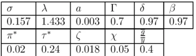
Following Cooley and Prescott (1995), we have setρ= 0.81, which reflects that 95 percent of the technology shock remains after one quarter. Respectively we setρg = 0.975according to Blanchard and Perotti (2002), which means that 95 percent of the government spending shock still remains after 2 years. The model is calibrated to reflect the economic structure of a large economy and the key parameter values of the model are given in Table 1.

Table 2 shows the steady state results with the debt rule (2.42) and discretionary monetary policy (2.31). We let the fiscal policy rule parameter

φvary from 0.1 to 1.5 and the debt to GDP ratio targetψ₁from a tight target

(0) to a loose target (1.5). As concluded in Railavo (2003 and 2004), the low values of the fiscal policy rule parameter indicate active fiscal policy while the higher values refer to passive policy. As defined in Leeper (1991), the passive fiscal policy authority must generate sufficient tax revenues to balance the

σ λ a Γ δ β 0.157 1.433 0.003 0.7 0.97 0.97

π∗ τ∗ ζ χ g_y

0.02 0.24 0.018 0.05 0.4

Table 1: The parameter values used and not altered in simulation

φ 0.1 0.5 0.9 1.5

ψ₁ mean mean mean mean

Inflation 00.6 1.5 5.1 5.8 7.1 4.9 5.1 5.3 4.9 5.0 5.1 4.9 4.9 5.0 Interest rate 0 0.6 1.5 8.6 9.3 10.6 8.4 8.6 8.8 8.4 8.5 8.6 8.4 8.4 8.5 Debt to GDP ratio 0 0.6 1.5 155.5 818.1 1812.2 20.3 145.5 333.2 6.2 75.3 179.0 −0.7 40.6 102.6 Tax rate 00.6 1.5 40.2 44.6 51.3 39.3 40.1 41.4 39.2 39.7 40.4 39.2 39.4 39.8

Table 2: Discretionary monetary policy with the debt rule

budget regardless of inflation, whereas the active authority is not constrained by budgetary conditions. Monetary policy is active with both discretionary and commitment monetary policy. The steady state values of the tax rules

(2.42) and (2.43) depend on the values of the fiscal policy parameter φ and

Ω, respectively, and also on the values of the target, ψ₁ and ψ₂, respectively. However, the steady state values of the tax rules (2.44) and (2.45) do not depend on the values of the fiscal policy parameterφ and Ω, respectively, but only on the values of the target, ψ₁ andψ₂, respectively.

We can see from Table 2 that there is inflation bias with discretionary monetary policy, as inflation is above the target value, π∗ = 0.02. We also see that the size of the bias depends on the fiscal policy parameter, φ, values and the debt to GDP target, ψ₁, values. Loosening the debt to GDP target increases the steady state debt to GDP ratio and the steady state inflation increases. The high tax rate is associated with the high debt to GDP ratios, which feeds into inflation. The debt to GDP ratio decreases as the fiscal policy parameter gets larger values, ie the fiscal policy authority reacts more with the tax rate. The largest changes in the steady state values happen when the fiscal policy parameter, φ, changes from 0.1 to 0.5. With higher values of φ, the change in the steady state values of inflation, the tax rate and the interest rate is small compared to the changes in the debt to GDP ratio. Also, with the φ = 0.1, the change in the target parameter has the largest impact on the steady state values of inflation and the tax rate. This indicates that there is strong non-linearity with the low values of φ.

Ω 0.1 0.5 0.9 1.5

ψ₂ mean mean mean mean

Inflation 0.003 0.1 9.0 9.5 10.6 5.4 5.5 5.7 5.1 5.2 5.3 5.1 5.1 5.2 Interest rate 0.003 0.1 12.5 13.0 14.0 8.9 9.0 9.2 8.6 8.7 8.8 8.5 8.6 8.6 Debt to GDP ratio 0 0.03 0.1 3120.0 3408.4 3976.3 443.8 529.8 712.5 228.6 274.3 378.5 128.9 156.1 218.7 Tax rate 0.003 0.1 60.0 61.9 65.7 42.1 42.7 43.9 40.7 41.0 41.7 40.0 40.2 40.6

Table 3: Discretionary monetary policy with the deficit rule

Table 3 shows the steady state ratios with the deficit rule (2.43). Now the deficit to GDP target ψ₂ gets values between zero and 0.1 as the fiscal policy rule parameter Ω runs from 0.1 to 1.5. Again, we see that increasing the target makes the debt to GDP ratio increase, which has an impact on inflation. We also see that the low values of the fiscal policy rule parameter result in an extremely high debt to GDP ratio in the steady state. The high debt levels are associated with the high tax rate and with the low fiscal policy parameter value. Overall, the debt and deficit rule results in similar steady state responses to changes in the fiscal policy parameter and target values.

Table 4 shows the steady state values under the deficit rule(2.45). Now the fiscal policy parameter Ω has an impact neither on the steady state tax rate nor on the steady state debt to GDP level. Increase in the deficit target ψ₂

increases the steady state debt to GDP ratio and inflation. However, changing the deficit target has a small effect on the level of the steady state inflation compared on the quite large impact to the debt to GDP ratio.

Tables 5 and 6 display the steady state values when the monetary policy authority is able to commit. As expected, inflation will be at the target level for all combinations of the fiscal policy parameter and the target values. With the debt rule (2.42), the debt to GDP ratio will increase as the fiscal policy parameter φ value decreases and the debt to GDP target ψ₁ value increases. With the error-correction deficit rule (2.45), the fiscal policy parameter does not have an effect on the steady state debt to GDP ratios. However, the debt to GDP ratio will increase as the deficit target increases, which results in a higher steady state tax rate.

Tables 7 to 11 display the variability and persistence statistics as a response to the underlying fundamental stochastic shocks. We let the fiscal policy parameters, φ and Ω, vary from 0.1 to 1.5 and the target parameter value changes from low (tight) to higher values (looser).

Barro (1979) claims that an optimal monetary and fiscal policy problem results in an optimal tax rate and debt will follow a random walk. Lucas and Stokey (1983) and Chari et al (1991 and 1994) show that with flexible

Ω 0.1 0.5 0.9 1.5

ψ₂ mean mean mean mean

Inflation 0.003 0.1 4.9 5.0 5.0 4.9 5.0 5.0 4.9 5.0 5.0 4.9 5.0 5.0 Interest rate 0 0.03 0.1 8.4 8.4 8.5 8.4 8.4 8.5 8.4 8.4 8.5 8.4 8.4 8.5 Debt to GDP ratio 0 0.03 0.1 −11.1 28.8 120.1 −11.1 28.8 120.1 −11.1 28.8 120.1 −11.1 28.8 120.1 Tax rate 0.003 0.1 39.1 39.4 40.0 39.1 39.4 40.0 39.1 39.4 40.0 39.1 39.4 40.0

Table 4: Discretionary monetary policy with the error-correction deficit rule

φ 0.1 0.5 0.9 1.5

ψ₁ mean mean mean mean

Inflation 00.6 1.5 2.0 2.0 2.0 2.0 2.0 2.0 2.0 2.0 2.0 2.0 2.0 2.0 Interest rate 00.6 1.5 5.5 5.5 5.5 5.5 5.5 5.5 5.5 5.5 5.5 5.5 5.5 5.5 Debt to GDP ratio 0 0.6 1.5 155.4 817.9 1811.6 18.5 143.5 331.1 4.2 73.2 176.8 −2.9 38.4 100.4 Tax rate 00.6 1.5 40.4 44.9 51.6 39.5 40.3 41.6 39.4 39.9 40.6 39.4 39.6 40.1

Ω 0.1 0.5 0.9 1.5

ψ₂ mean mean mean mean

Inflation 0.003 0.1 2.0 2.0 2.0 2.0 2.0 2.0 2.0 2.0 2.0 2.0 2.0 2.0 Interest rate 0.003 0.1 5.5 5.5 5.5 5.5 5.5 5.5 5.5 5.5 5.5 5.5 5.5 5.5 Debt to GDP ratio 0 0.03 0.1 −13.4 51.0 201.3 −13.4 51.0 201.3 −13.4 51.0 201.3 −13.4 51.0 201.3 Tax rate 0.003 0.1 39.3 39.7 40.7 39.3 39.7 40.7 39.3 39.7 40.7 39.3 39.7 40.7

Table 6: Committed monetary policy with the error-correction deficit rule

prices Barro’s result of an optimal tax rate to follow a random walk does not hold. Chari et al (1991 and 1994) also claim that the tax rate and debt inherit the serial correlation of the model’s underlying shocks. Siu (2004) found that in a sticky price model, especially in the case in which government finances spending by increasing taxes, resulting in an accumulated debt, the autocorrelations of the debt to GDP ratio and the tax rate are near unity regardless of the persistence in the shock process, partially reviving Barro’s random walk result.

In Table 7 we can see that the variability of inflation decreases as the parameter φ in the debt rule (2.42) gets larger values, but the variability of the tax rate increases. The variability of both inflation and the tax rate increases as the debt to GDP ratio target, ψ₁, gets larger values. Inflation and the interest rate are highly autocorrelated for all the parameter values. The persistence of the debt to GDP ratio and the tax rate decreases as both or either the fiscal policy parameter and the debt to GDP ratio target get larger values. With the low target values, ie the low steady state debt to GDP ratio, the autocorrelation of the debt to GDP ratio and the tax rate are near unity supporting Barro’s (1979) result. However, increasing the target values, ie making the debt to GDP ratio less restrictive, reduces the autocorrelation of the variables and supports the Chari et al (1991 and 1994) result even in a sticky price model. Output variability and persistence remain quite constant and low regardless of the changes in the parameter values.

Table 8 repeats the previous results now with the deficit rule (2.43). The overall results are similar to the previous results, but the persistence of the debt to GDP ratio and the tax rate do not decrease with the increase of the values of theΩandψ₂ parameters. Now we find support for Barro (1979) and Siu (2004) with all parameter value combinations. The change in fiscal policy do not affect the persistence of the tax rate. However, output persistence and volatility do not improve due to results with the debt rule.

The introduction of the error-correction deficit rule (2.45) does not change the results significantly compared with the deficit rule(2.43), as can be seen in

Table 9. The persistence of inflation, the interest rate, the debt to GDP ratio and the tax rate remains high. However, the variability of inflation decreases with the low fiscal policy parameter Ω values compared with the results of the deficit rule. This is due to the fact that the fiscal policy parameter has no impact on the debt to GDP ratio and hence on the level of inflation with the error-correction deficit rule. The variability of the debt to GDP ratio is smaller when the debt to GDP ratio level is smaller.

In Table 10 we see the results with committed monetary policy(2.39) and the debt rule (2.42). We can see that under the commitment of monetary policy output persistence increases significantly compared to the discretionary case. This demonstrates the timeless perspective of monetary policy as optimal monetary policy under commitment(2.40)displays a lagged inflation term. As the persistence increases there is a considerable increase in the variability of output. Whereas the variability of output increases under commitment, that of inflation and the interest rate falls. The variability of the tax rate and the debt to GDP ratio remain relatively similar with both discretionary and committed monetary policy. However, the persistence of the two increases somewhat, especially with the high fiscal policy and debt to GDP ratio target values. Still, the autocorrelation of the two variables gives support to the Barro finding when the target has low values. As the debt to GDP increases and the fiscal policy reacts more with taxes, the autocorrelation drops and the tax rate inherits the serial correlation of the shock as in Chari et al (1991 and 1994).

The same result shows up with the deficit rule (2.45). The results inTable 11 are similar to the results of discretionary monetary policy with the deficit rule except for output. Like in the previous case, the volatility and persistence of output has increased significantly compared with the discretionary monetary policy case. The autocorrelation of the debt to GDP ratio and the tax rate will remain high, reflecting Barro’s results with all the fiscal parameter combinations.

4 Conclusions

In this paper we analysed the effects of alternative fiscal policy rules with optimal monetary policy. With discretionary monetary policy, inflation bias depends on the fiscal policy with both the debt and deficit rule. The fiscal policy parameter and the target values, hence the fiscal policy regime, affect the size of the bias. The higher values the fiscal policy parameter and the target parameter get the higher the steady state debt to GDP ratio is and inflation becomes. The target parameter changes increase inflation more evenly, but the policy parameter changes are more notable between low values than with high values.

With the error-correction deficit rule, the fiscal policy parameter has no impact on the steady state tax rate and, also, on the steady state debt to GDP level. A rise in the deficit target increases the steady state debt to GDP ratio and inflation. However, changing the deficit target has a small effect on

the level of the steady state inflation compared to the quite large impact on the debt to GDP ratio.

The stochastic simulation results show that under central bank commitment, output persistence increases compared to the discretionary case. The result is derived using the timeless perspective approach to precommitment by Woodford (1999). Under the timeless perspective, inflation and output persistence reflects the economic data. The fiscal policy is also compatible with the optimal monetary policy from timeless a perspective and the result holds also with alternative fiscal policy rules. The fiscal policy parameter and the target values do not affect the persistence of inflation and output. However, the variability of output increases compared to the discretionary case.

With the deficit rules, the autocorrelation of the tax rate is near unity irrespective of the monetary policy regime, and irrespective of the fiscal policy parameters and targets. Thus we revive Barro’s (1979) random walk result with the deficit rules. With the debt rules and the high debt to GDP target values, the Barro result does not hold and the tax rate inherits the stochastic nature of underlying shocks. With the error-correction type of fiscal policy rule, the tax rate changes are smooth as the autocorrelation is near unity with all combinations of the fiscal policy parameter and the deficit to GDP target values.

References

Aiyagari, S.R. — Marcet, A. — Sargent, T.J. — Seppälä, J. (2002) Optimal Taxation without State-Contingent Debt.Journal of Political Economy, Vol. 110, No. 6, 1220—1254.

Aoki, K. — Nikolov, K. (2003) Rule-Based Monetary Policy Under Central Bank Learning. Paper held at Bank of Finland/CEPR Annual Workshop, Helsinki, 2/3 October 2003.

Barro, R.J. (1979) On Determination of the Public Debt. Journal of Political Economy, Vol. 87, Issue 5, Part 1, 940—971.

Barro, R.J. — Gordon, D.B. (1983)A Positive Theory of Monetary Policy in a Natural Rate Model. Journal of Political Economy, Vol. 91, No. 4, 589—610.

Benhabib, J. — Wen, Y. (2004) Indeterminacy, Aggregate Demand, and the Real Business Cycle. Journal of Monetary Economics 51, 503—530.

Blanchard, O. — Perotti, R. (2002) An Empirical Characterization of the Dynamic Effects of Changes in Government Spending and Taxes on Output. Quarterly Journal of Economics, November, 1329—1368.

Chari, V.V. — Christiano, L.J. — Kehoe, P.J. (1991) Optimal Fiscal and Monetary Policy: Some Recent Results. Journal of Money, Credit and Banking, Vol. 23, Issue 3, Part 2, 519—539.

Chari, V.V. — Christiano, L.J. — Kehoe, P.J. (1994) Optimal Fiscal Policy in a Business Cycle Model. The Journal of Political Economy, Vol. 102, Issue 4, 617—652.

Cooley, T.F. — Prescott, E.C. (1995) Economic Growth and Business Cycles.In Cooley, T.F. (Ed.) Frontiers of Business Cycle Research, Princeton University Press.

Cukierman, A. (1992) Central Bank Strategy, Credibility and Independence: Theory and Evidence.MIT Press.

Leeper, E.M. (1991) Equilibria under ‘Active’ and ‘Passive’ Monetary and Fiscal Policies. Journal of Monetary Economics 27, 129—147.

Lucas, R.E. — Stokey, N.L. (1983)Optimal Fiscal and Monetary Policy in an Economy without Capital. Journal of Monetary Economics 12, 55—93.

Railavo, J. (2003) Effects of the Supply-side Channel on Stabilisation Properties of Policy Rules. Bank of Finland Discussion Papers 34/2003.

Railavo, J. (2004) Stability Consequences of Fiscal Policy Rules. Bank of Finland Discussion Papers 1/2004.

Rogoff, K. (1985) The Optimal Degree of Commitment to an Intermediate Monetary Target. Quarterly Journal of Economics, November, 1169—1189.

Rotemberg, J.J. (1987)The New Keynesian Microfoundations.In Fisher, S. (Ed.) NBER Macroeconomic Annual, MIT Press.

Rotemberg, J.J. — Woodford, M. (1998) An Optimization-Based Econometric Framework for the Evaluation of Monetary Policy: Expanded Version. NBER Technical Working Paper 233.

Sargent, T.J. — Wallace, N. (1981) Some Unpleasant Monetarist Arithmetic. Federal Reserve Bank of Minneapolis Quarterly Review, Vol. 5, No. 3, 1—17.

Schmitt-Grohé, S. — Uribe, M. (2003)Optimal Simple and Implementable Monetary and Fiscal Rules. Mimeo Duke University. Available at http://www.econ.duke.edu/~grohe/

Schmitt-Grohé, S. — Uribe, M. (2004a) Optimal Fiscal and Monetary Policy Under Sticky Prices. Journal of Economic Theory, 198—230.

Schmitt-Grohé, S. — Uribe, M. (2004b) Optimal Fiscal and Monetary Policy Under Imperfect Competition. Journal of Macroeconomics, 183—209.

Siu, H.E. (2004) Optimal Fiscal and Monetary Policy with Sticky Prices. Journal of Monetary Economics 51, 575—607.

Svensson, L.E.O. (1997) Optimal Inflation Targets, ‘Conservative’ Central Banks, and Linear Inflation Contracts. American Economic Review, Vol. 87, No. 1, 98—114.

Taylor, J.B. (1993) Discretion versus Policy Rules in Practice. Carnegie-Rochester Conference Series on Public Policy 39, 195—214.

Woodford, M. (1999) Optimal Monetary Policy Inertia. Manchester School Supplement, 1—35.

Woodford, M. (2003) Interest and Prices. Foundations of a Theory of Monetary Policy. Princeton University Press.

Appendix A1 Potential output without distortionary

taxes

Let’s rewrite the household’s budget constraint with lump sum taxation

c_t+m_t−(1−π_t)m_t−1+b_t ≤(1 +r_t−1)b_t−1+w_tl_t−T_t, (4.1) where T_t is lump sum taxes. Now the household’s utility maximisation using the periodic utility functionu(c_t, m_t, l_t;g_t) = c1−σt

1−σ +Γm 1−σ t 1−σ −l 1+λ t 1+λ+f(gt)yields

a first order condition for the labour supply

−lλt=−c−_tσwt. (4.2)

The real marginal cost to the cost minimising firm is

∂ ∂y_t wt yt A =wt1 A =mct. (4.3)

With equilibrium wages wt =cσtyt

Aλ the real marginal cost is

cσtyλtA−(1+λ)=mct. (4.4)

In order to log-linearise (4.4), first substitute in the process for technological progress A = Λteζ∗Time and take natural logarithms. Use the definition xt = ln (xt/x) and substitute in the resource constraint ct = y_cyt−g_cgt to yield

σy c +λ yt−σg cgt−(1 +λ)Λt=mct. (4.5)

In a flexible price equilibrium we get the long-run supply function to look like

lny_t∗= σ g c κ lngt+ 1 +λ κ ζ∗T ime+ε y∗ t , (4.6)

wherey∗_t is the level of flexible price output, which is the desired level of output for the central bank, κ = σy_c +λ and εy_t∗ = 1+λ_κ z_t.10 As we can see from

(2.21) and (4.6), the long-run flexible price output and the desired level of output are both hit by the same technology shock(2.3).

φ 0.1 0.5 0.9 1.5 ψ₁ std (corr.) std (corr.) std (corr.) std (corr.) Inflation 0 − 0.6 − 1.5 − 0.5047 (0.9878) 0.5553 (0.9887) 0.6715 (0.9902) 0.4514 (0.9782) 0.4026 (0.9756) 0.4506 (0.9807) 0.4212 (0.9761) 0.4010 (0.9726) 0.4235 (0.9753) 0.4226 (0.9741) 0.4573 (0.9790) 0.4069 (0.9731) Interest rate 0 − 0.6 − 1.5 − 0.5289 (0.9793) 0.5762 (0.9807) 0.6952 (0.9818) 0.4514 (0.9726) 0.4221 (0.9665) 0.4714 (0.9724) 0.4390 (0.9692) 0.4192 (0.9654) 0.4445 (0.9599) 0.4226 (0.9652) 0.4804 (0.9683) 0.4262 (0.9667) Output 0 − 0.6 − 1.5 − 1.6657 (0.1875) 1.6875 (0.1221) 1.6886 (0.1729) 1.7173 (0.1914) 1.6535 (0.1675) 1.6862 (0.1662) 1.6566 (0.1697) 1.6305 (0.1288) 1.6428 (0.1615) 1.6850 (0.1593) 1.7114 (0.2262) 1.6436 (0.1647) Debt to GDP ratio 0 − 0.6 − 1.5 − 45.560 (0.9959) 45.808 (0.9240) 54.799 (0.7774) 10.809 (0.9904) 9.5861 (0.9662) 10.767 (0.8929) 6.1155 (0.9797) 5.8572 (0.9762) 6.2774 (0.9746) 4.3282 (0.9465) 4.8640 (0.9234) 4.4393 (0.7539) Tax rate 0 − 0.6 − 1.5 − 4.3275 (0.9950) 4.4212 (0.9022) 5.4342 (0.7192) 4.6883 (0.9870) 4.3136 (0.8768) 5.3802 (0.6182) 4.4138 (0.9719) 4.4687 (0.8059) 5.5870 (0.4685) 4.6699 (0.9147) 5.5601 (0.6704) 6.5240 (0.0470)

Table 7: Discretionary monetary policy with the debt rule Note: corr. is the first-order autocorrelation coefficient.

Ω 0.1 0.5 0.9 1.5 ψ₂ std (corr.) std (corr.) std (corr.) std (corr.) Inflation 0 − 0.03 − 0.1 − 0.7794 (0.9932) 0.8580 (0.9910) 0.8019 (0.9834) 0.5291 (0.9894) 0.5289 (0.9888) 0.5130 (0.9877) 0.4189 (0.9801) 0.3959 (0.9781) 0.5292 (0.9869) 0.4229 (0.9785) 0.3901 (0.9762) 0.3927 (0.9753) Interest rate 0 − 0.03 − 0.1 − 0.8012 (0.9870) 0.8773 (0.9848) 0.8196 (0.9752) 0.5523 (0.9817) 0.5535 (0.9823) 0.5366 (0.9810) 0.4381 (0.9709) 0.4144 (0.9681) 0.5523 (0.9821) 0.4423 (0.9708) 0.4097 (0.9660) 0.4132 (0.9594) Output 0 − 0.03 − 0.1 − 1.6827 (0.1909) 1.6832 (0.1423) 1.6987 (0.1523) 1.7118 (0.1533) 1.6855 (0.2103) 1.6764 (0.2090) 1.6087 (0.1326) 1.6021 (0.1035) 1.6866 (0.2062) 1.6302 (0.1341) 1.6675 (0.1663) 1.6796 (0.1312) Debt to GDP ratio 0 − 0.03 − 0.1 − 148.53 (0.9073) 114.93 (0.7975) 84.717 (0.5051) 74.916 (0.9898) 64.706 (0.9850) 62.420 (0.9720) 37.169 (0.9898) 32.066 (0.9809) 39.342 (0.9788) 24.766 (0.9915) 22.272 (0.9867) 19.857 (0.9680) Tax rate 0 − 0.03 − 0.1 − 3.8454 (0.9658) 4.0399 (0.9497) 3.7197 (0.9007) 4.2277 (0.9900) 4.0738 (0.9882) 4.2073 (0.9836) 3.6168 (0.9851) 3.3538 (0.9809) 4.6444 (0.9874) 3.9187 (0.9844) 3.6504 (0.9818) 3.7104 (0.9778)

Table 8: Discretionary monetary policy with the deficit rule Note: corr. is the first-order autocorrelation coefficient.

Ω 0.1 0.5 0.9 1.5 ψ₂ std (corr.) std (corr.) std (corr.) std (corr.) Inflation 0 − 0.03 − 0.1 − 0.4674 (0.9808) 0.4251 (0.9774) 0.4796 (0.9805) 0.4140 (0.9735) 0.3737 (0.9679) 0.4303 (0.9734) 0.4352 (0.9757) 0.4376 (0.9755) 0.4100 (0.9708) 0.4782 (0.9802) 0.4281 (0.9750) 0.4069 (0.9709) Interest rate 0 − 0.03 − 0.1 − 0.4867 (0.9751) 0.4472 (0.9568) 0.5036 (0.9623) 0.4326 (0.9678) 0.3915 (0.9599) 0.4482 (0.9661) 0.4512 (0.9669) 0.4595 (0.9698) 0.4269 (0.9609) 0.4982 (0.9755) 0.4487 (0.9683) 0.4271 (0.9585) Output 0 − 0.03 − 0.1 − 1.6460 (0.1589) 1.6747 (0.1082) 1.6737 (0.2108) 1.6394 (0.1340) 1.6865 (0.1575) 1.7057 (0.1813) 1.6189 (0.1312) 1.6259 (0.1759) 1.6621 (0.0989) 1.7167 (0.2000) 1.7191 (0.1870) 1.6883 (0.1696) Debt to GDP ratio 0 − 0.03 − 0.1 − 22.773 (0.9937) 22.228 (0.9934) 24.924 (0.9896) 4.9277 (0.9756) 4.8715 (0.9602) 7.0619 (0.9117) 3.0851 (0.9637) 3.1398 (0.9314) 5.6452 (0.8615) 2.3736 (0.9583) 2.1743 (0.8753) 5.4831 (0.8614) Tax rate 0 − 0.03 − 0.1 − 4.7344 (0.9980) 4.3486 (0.9964) 5.1300 (0.9969) 4.3898 (0.9947) 4.1160 (0.9933) 4.7837 (0.9936) 4.6198 (0.9925) 4.8095 (0.9923) 4.4812 (0.9895) 5.2316 (0.9924) 4.8055 (0.9894) 4.5675 (0.9858)

Table 9: Discretionary monetary policy with the error-correction deficit rule Note: corr. is the first-order autocorrelation coefficient.

φ 0.1 0.5 0.9 1.5 ψ₁ std (corr.) std (corr.) std (corr.) std (corr.) Inflation 0 − 0.6 − 1.5 − 0.3780 (0.9993) 0.3780 (0.9993) 1.1061 (0.9993) 0.2664 (0.9989) 0.4790 (0.9994) 0.3506 (0.9980) 0.3368 (0.9993) 0.3899 (0.9991) 0.4140 (0.9985) 0.4088 (0.9994) 0.2716 (0.9980) 0.4772 (0.9981) Interest rate 0 − 0.6 − 1.5 − 0.3762 (0.9712) 0.3762 (0.9891) 1.0428 (0.9957) 0.2655 (0.9505) 0.4619 (0.9789) 0.3385 (0.9804) 0.3313 (0.9560) 0.3782 (0.9813) 0.4022 (0.9719) 0.3914 (0.9810) 0.2649 (0.9685) 0.4595 (0.9862) Output 0 − 0.6 − 1.5 − 5.3338 (0.9300) 5.3338 (0.9354) 9.2104 (0.9470) 3.7499 (0.8590) 6.1079 (0.9473) 4.7310 (0.8995) 4.6285 (0.9099) 5.0139 (0.9154) 5.5182 (0.9326) 5.6589 (0.9373) 3.9712 (0.8751) 6.0799 (0.9433) Debt to GDP ratio 0 − 0.6 − 1.5 − 55.867 (0.9967) 51.656 (0.9381) 79.207 (0.7823) 8.8037 (0.9853) 11.2068 (0.9704) 10.593 (0.8837) 7.3973 (0.9840) 6.4000 (0.9769) 6.1636 (0.9669) 4.8565 (0.9607) 3.9692 (0.9080) 4.6603 (0.8086) Tax rate 0 − 0.6 − 1.5 − 5.3254 (0.9965) 4.9912 (0.9251) 8.0805 (0.7601) 3.8769 (0.9852) 5.1570 (0.9201) 5.3370 (0.6447) 5.4214 (0.9826) 4.9484 (0.8696) 5.6354 (0.5486) 5.4925 (0.9490) 4.8087 (0.6558) 6.9800 (0.2226)

Table 10: Committed monetary policy with the debt rule Note: corr. is the first-order autocorrelation coefficient.

Ω 0.1 0.5 0.9 1.5 ψ₂ std (corr.) std (corr.) std (corr.) std (corr.) Inflation 0 − 0.03 − 0.1 − 0.4174 (0.9994) 0.3110 (0.9988) 0.3112 (0.9989) 0.4230 (0.9995) 0.4737 (0.9996) 0.2766 (0.9988) 0.3455 (0.9993) 0.2230 (0.9984) 0.2489 (0.9986) 0.3468 (0.9994) 0.3328 (0.9993) 0.4017 (0.9994) Interest rate 0 − 0.03 − 0.1 − 0.4103 (0.9767) 0.3134 (0.9678) 0.3124 (0.9628) 0.4106 (0.9759) 0.4595 (0.9714) 0.2741 (0.9483) 0.3349 (0.9704) 0.2255 (0.9163) 0.2466 (0.9472) 0.3340 (0.9745) 0.3223 (0.9733) 0.3907 (0.9627) Output 0 − 0.03 − 0.1 − 5.0627 (0.9248) 3.6744 (0.8536) 4.0660 (0.8660) 5.2468 (0.9274) 5.8583 (0.9439) 4.3010 (0.8868) 4.6996 (0.9073) 3.3931 (0.8247) 3.7303 (0.8459) 4.7477 (0.9169) 4.6473 (0.9074) 5.5021 (0.9225) Debt to GDP ratio 0 − 0.03 − 0.1 − 27.826 (0.9959) 27.942 (0.9941) 27.762 (0.9826) 6.2676 (0.9833) 9.7789 (0.9776) 13.558 (0.9348) 3.5880 (0.9724) 4.7642 (0.9330) 11.224 (0.9192) 2.4566 (0.9615) 5.0680 (0.9505) 13.401 (0.9622) Tax rate 0 − 0.03 − 0.1 − 4.5000 (0.9985) 4.6680 (0.9979) 4.2214 (0.9979) 4.7386 (0.9949) 4.9807 (0.9950) 5.0815 (0.9943) 4.5033 (0.9924) 3.8388 (0.9881) 3.8992 (0.9870) 4.2570 (0.9876) 4.5649 (0.9887) 4.9495 (0.9891)

Table 11: Committed monetary policy with the error-correction deficit rule Note: corr. is the first-order autocorrelation coefficient.

BANK OF FINLAND DISCUSSION PAPERS

ISSN 0785-3572, print; ISSN 1456-6184, online

1/2004 Jukka Railavo Stability consequences of fiscal policy rules. 2004. 42 p. ISBN 952-462-114-2, print; ISBN 952-462-115-0, online. (TU)

2/2004 Lauri Kajanoja Extracting growth and inflation expectations from financial market data. 2004. 25 p. ISBN 952-462-116-9, print; ISBN 952-462-117-7, online. (TU)

3/2004 Martin Ellison – Lucio Sarno – Jouko Vilmunen Monetary policy and learning in an open economy. 2004. 24 p. ISBN 952-462-118-5, print; ISBN 952-462-119-3, online. (TU)

4/2004 David G. Mayes An approach to bank insolvency in transition and emerging economies. 2004. 54 p. ISBN 952-462-120-7, print;

ISBN 952-462-121-5, online. (TU)

5/2004 Juha Kilponen Robust expectations and uncertain models – A robust control approach with application to the New Keynesian economy. 2004. 43 p. ISBN 952-462-122-3, print; ISBN 952-462-123-1, online. (TU)

6/2004 Erkki Koskela – Roope Uusitalo Unintended convergence – how Finnish unemployment reached the European level. 2004. 32 p.

ISBN 952-462-124-X, print; ISBN 952-462-125-8, online. (TU)

7/2004 Berthold Herrendorf – Arilton Teixeira Monopoly rights can reduce income big time. 2004. 38 p. ISBN 952-462-126-6, print; ISBN 952-462-127-4, online. (TU)

8/2004 Allen N. Berger – Iftekhar Hasan – Leora F. Klapper Further evidence on the link between finance and growth: An international analysis of community banking and economic performance. 2004. 50 p. ISBN 952-462-128-2, print; ISBN 952-462-129-0, online. (TU)

9/2004 David G. Mayes – Matti Virén Asymmetries in the Euro area economy.

2004. 56 p. ISBN 952-462-130-4, print; ISBN 952-462-131-2, online. (TU) 10/2004 Ville Mälkönen Capital adequacy regulation and financial conglomerates.

11/2004 Heikki Kauppi – Erkki Koskela – Rune Stenbacka Equilibrium unemployment and investment under product and labour market

imperfections. 2004. 35 p. ISBN 952-462-136-3, print; ISBN 952-462-137-1, online. (TU)

12/2004 Nicolas Rautureau Measuring the long-term perception of monetary policy and the term structure. 2004. 44 p. ISBN 952-462-138-X, print;

ISBN 952-462-139-8, online. (TU)

13/2004 Timo Iivarinen Large value payment systems – principles and recent and future developments. 2004. 57 p. ISBN 952-462-144-4, print,

ISBN 952-462-145-2, online (RM)

14/2004 Timo Vesala Asymmetric information in credit markets and entrepreneurial risk taking. 2004. 31 p. 952-462-146-0, print, ISBN 952-462-147-9, online (TU)

15/2004 Michele Bagella – Leonardo Becchetti – Iftekhar Hasan The anticipated and concurring effects of the EMU: exchange rate volatility, institutions and growth. 2004. 38 p. 952-462-148-7, print, ISBN 952-462-149-5, online (TU)

16/2004 Maritta Paloviita – David G. Mayes The use of real time information in Phillips curve relationships for the euro area. 2004. 51 p. 952-462-150-9, print, ISBN 952-462-151-7, online (TU)

17/2004 Ville Mälkönen The efficiency implications of financial conglomeration.

2004. 30 p. 952-462-152-5, print, ISBN 952-462-153-3, online (TU)

18/2004 Kimmo Virolainen Macro stress testing with a macroeconomic credit risk model for Finland. 2004. 44 p. 952-462-154-1, print, ISBN 952-462-155-X, online (TU)

19/2004 Eran A. Guse Expectational business cycles. 2004. 34 p. 952-462-156-8, print, ISBN 952-462-157-6, online (TU)

20/2004 Jukka Railavo Monetary consequences of alternative fiscal policy rules.