MULTIPLE INSTANCE CHOQUET INTEGRAL
FOR MULTIRESOLUTION SENSOR FUSION
A Dissertation presented to the Faculty of the Graduate School
at the University of Missouri
In Partial Fulfillment
of the Requirements for the Degree Doctor of Philosophy
by XIAOXIAO DU
Dr. Alina Zare, Dissertation Supervisor DECEMBER 2017
The undersigned, appointed by the Dean of the Graduate School, have examined the dissertation entitled:
MULTIPLE INSTANCE CHOQUET INTEGRAL FOR MULTIRESOLUTION SENSOR FUSION
presented by Xiaoxiao Du,
a candidate for the degree of Doctor of Philosophy and hereby certify that, in their opinion, it is worthy of acceptance. Dr. Alina Zare Dr. James Keller Dr. Dominic Ho Dr. Marjorie Skubic Dr. Mihail Popescu
To my family, all my love.
ACKNOWLEDGMENTS
I would like to thank my dissertation adviser and committee chair, Dr. Alina Zare, for her wholehearted guidance, support, and all the opportunities she provided me throughout my studies and research. I am inspired by her dedication, passion, and creativity in research and teaching; I admire and respect her confidence, intelligence, and strength of character.
I would also like to thank my doctoral committee members, Dr. James Keller, Dr. Dominic Ho, Dr. Marjorie Skubic, and Dr. Mihail Popescu, for their help and valuable suggestions. I gained knowledge and experience in the lectures, seminars, and discussions, for which I am grateful.
Thank you to those who shed light on the field of multiple instance learning, computa-tional intelligence, and sensor fusion. Thank you to those who make the data sets used in this dissertation available.
I am thankful for the University of Missouri and Zhejiang University, for preparing me for the journey. I am thankful for my current and former teachers and professors, for their help and support along the way.
I am thankful for my labmates, for the times they provided insightful comments as well as encouragements in my studies and in life. I am grateful for my friends, for all the music and laughter.
Finally, a warm thank you goes to my parents and all of my family, for their love, support, understanding, and inspiration, as always.
TABLE OF CONTENTS
ACKNOWLEDGMENTS . . . ii
LIST OF TABLES . . . vi
LIST OF FIGURES . . . ix
LIST OF ABBREVIATIONS AND ACRONYMS . . . xvii
LIST OF SYMBOLS AND NOTATIONS . . . xix
ABSTRACT . . . xx
CHAPTER 1 Introduction . . . 1
2 Literature Review . . . 6
2.1 Multiple Instance Classification . . . 6
2.2 Multiple Instance Regression . . . 13
2.3 Fuzzy Measure and Choquet Integral . . . 19
2.3.1 Fuzzy Measure . . . 20
2.3.2 Choquet Integral . . . 22
2.3.3 Learning The Fuzzy Measure . . . 24
2.4 Sensor Fusion . . . 32
2.4.1 Co-registration . . . 33
2.5 Summary and Discussion of Literature Review . . . 42
3 Multiple Instance Choquet Integral . . . 45
3.1 Noisy-or Model . . . 46
3.2 Min-Max Model . . . 47
3.3 Generalized Mean Model . . . 48
3.4 Optimization . . . 50
3.4.1 Measure Initialization . . . 50
3.4.2 Evaluation of Valid Intervals . . . 52
3.4.3 Mutation . . . 53
3.4.4 Selection . . . 54
4 Multiple Instance Choquet Integral Regression . . . 56
5 Multi-Resolution Multiple Instance Choquet Integral . . . 58
6 Experimental Results . . . 62
6.1 Classification . . . 62
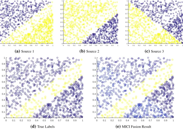
6.1.1 Synthetic 3-Source Classification Data Set . . . 63
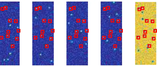
6.1.2 Synthetic Lane-Based Target Detection Data Set . . . 64
6.1.3 Synthetic 5-Source Classification Data Set For Varying Parameters . 67 6.1.4 MUUFL Gulfport Target Detection . . . 69
6.2 Multi-Resolution Fusion Data Set . . . 104
6.2.1 Synthetic Multi-Resolution Fusion Data Set . . . 104
6.2.2 MUUFL Gulfport Building Detection – Sub-image . . . 107
6.2.3 MUUFL Gulfport Scene Understanding: Building, Sidewalk and Road . . . 108
6.2.4 Soybean and Weed Data Set . . . 115
6.3 Regression Data Set . . . 137
6.3.1 Synthetic Regression Data Set . . . 137
6.3.2 Crop Yield Data Set . . . 139
6.4 Discussion on Optimization Schemes . . . 144
6.4.1 “Top-Down” and “Bottom-Up” Initialization . . . 144
6.4.2 Sampling according to measure element used . . . 145
6.4.3 Using a binary fuzzy measure . . . 148
7 Conclusion . . . 157
APPENDIX A Truncated Gaussian Sampling Method . . . 159
BIBLIOGRAPHY . . . 162
LIST OF TABLES
Table
Page
6.1 Mean and standard deviation of estimated and true measure element values learned by MICI noisy-or model for synthetic 3-source MICI classification data set over three runs. . . 65 6.2 Mean and the standard deviation (in parentheses) of estimated measure
el-ement values learned for synthetic 5-source lane-based classification data set over five runs. . . 68 6.3 The positive detection and false alarm rate of the synthetic lane-based target
detection data set after five-fold cross validation across five runs. . . 70 6.4 Relative error versus contamination for synthetic classification data set for
MICI noisy-or model across five runs. . . 70 6.5 Relative error versus contamination for synthetic classification data set for
MICI min-max model across five runs. . . 71 6.6 Relative error versus contamination for synthetic classification data set for
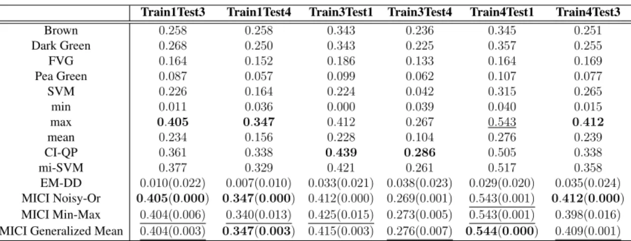
MICI generalized mean model across five runs. . . 71 6.7 The AUC results at on un-normalized MUUFL Gulfport data across five
6.8 The AUC results at on normalized MUUFL Gulfport data across five runs. Normalized by dividing over the norm of the data. . . 77 6.9 The AUC results at on normalized MUUFL Gulfport data across five runs.
Normalized by unity-based normalization. . . 78 6.10 The AUC results at on normalized MUUFL Gulfport data across five runs.
Normalized by the mean and standard deviation. . . 79 6.11 Running time (seconds) and number of iterations until convergence for
MICI models comparison. . . 79 6.12 One example estimated measure element values learned for synthetic
5-source multi-resolution classification data set after one run. . . 106 6.13 The AUC results of building, sidewalk, and road detection using MUUFL
Gulfport HSI and LiDAR data. . . 114 6.14 The RMSE results of MICI and MR-MICI on building, sidewalk, and road
detection. . . 114 6.15 The AUC and RMSE results of MICI and MR-MICI on building detection,
scored on edges. Train on campus 1 and test on campus 2. . . 115 6.16 The AUC and RMSE results of MICI and MR-MICI on building detection,
scored on edges. Train on campus 2 and test on campus 1. . . 115 6.17 Relative error versus percentage of primary instances for synthetic
regres-sion data set for MICI Regresregres-sion model across five runs. . . 138 6.18 Relative error versus SNR for synthetic regression data set MICI
Regres-sion model across five runs. . . 139 6.19 Number of counties (bags) with both corn and wheat yield in the crop yield
6.20 RMSE error for CA corn and wheat yield, Training on Years 2001-2004, Test on Year 2005. . . 140 6.21 RMSE error for KS corn and wheat yield, Training on Year 2001-2004,
Test on Year 2005. . . 141 6.22 Running time (seconds) and number of iterations until convergence for
op-timization schemes comparison. . . 147 6.23 Running time (seconds) and number of iterations until convergence for
LIST OF FIGURES
Figure
Page
2.1 Illustration of bags in multiple instance learning. . . 7 2.2 Illustration of standard supervised classification, multiple instance learning
classification and embedded multiple instance learning classification. . . 8 2.3 An illustration for the subset and superset relationships between fuzzy
mea-sure elements given four sources. . . 21 5.1 Illustration for HSI and LiDAR fusion. . . 60 6.1 Synthetic 3-source dataset and results for MICI classifier fusion model. . . . 64 6.2 Colorbar. . . 65 6.3 One example of the synthetic lane-based target detection data set. . . 66 6.4 RX detection output (plotted horizontally) of the synthetic lane-based target
detection data set. . . 67 6.5 Relationship of fitness values vs. number of iterations in the synthetic
lane-based target detection experiment. . . 69 6.6 The RGB image from MUUFL Gulfport “campus 3” data set. . . 72
6.8 ROC curve results for the MUUFL Gulfport data when training on Campus 1 and testing on Campus 3. The HSI data were un-normalized. . . 80 6.9 ROC curve results for the MUUFL Gulfport data when training on Campus
1 and testing on Campus 4. The HSI data were un-normalized. . . 81 6.10 ROC curve results for the MUUFL Gulfport data when training on Campus
3 and testing on Campus 1. The HSI data were un-normalized. . . 82 6.11 ROC curve results for the MUUFL Gulfport data when training on Campus
3 and testing on Campus 4. The HSI data were un-normalized. . . 83 6.12 ROC curve results for the MUUFL Gulfport data when training on Campus
4 and testing on Campus 1. The HSI data were un-normalized. . . 84 6.13 ROC curve results for the MUUFL Gulfport data when training on Campus
4 and testing on Campus 3. The HSI data were un-normalized. . . 85 6.14 ROC curve results for the MUUFL Gulfport data when training on Campus
1 and testing on Campus 3. The HSI data were normalized by dividing over the norm of the data. . . 86 6.15 ROC curve results for the MUUFL Gulfport data when training on Campus
1 and testing on Campus 4. The HSI data were normalized by dividing over the norm of the data. . . 87 6.16 ROC curve results for the MUUFL Gulfport data when training on Campus
3 and testing on Campus 1. The HSI data were normalized by dividing over the norm of the data. . . 88 6.17 ROC curve results for the MUUFL Gulfport data when training on Campus
3 and testing on Campus 4. The HSI data were normalized by dividing over the norm of the data. . . 89
6.18 ROC curve results for the MUUFL Gulfport data when training on Campus 4 and testing on Campus 1. The HSI data were normalized by dividing over the norm of the data. . . 90 6.19 ROC curve results for the MUUFL Gulfport data when training on Campus
4 and testing on Campus 3. The HSI data were normalized by dividing over the norm of the data. . . 91 6.20 ROC curve results for the MUUFL Gulfport data when training on Campus
1 and testing on Campus 3. The HSI data were normalized by unity-based normalization. . . 92 6.21 ROC curve results for the MUUFL Gulfport data when training on Campus
1 and testing on Campus 4. The HSI data were normalized by unity-based normalization. . . 93 6.22 ROC curve results for the MUUFL Gulfport data when training on Campus
3 and testing on Campus 1. The HSI data were normalized by unity-based normalization. . . 94 6.23 ROC curve results for the MUUFL Gulfport data when training on Campus
3 and testing on Campus 4. The HSI data were normalized by unity-based normalization. . . 95 6.24 ROC curve results for the MUUFL Gulfport data when training on Campus
4 and testing on Campus 1. The HSI data were normalized by unity-based normalization. . . 96 6.25 ROC curve results for the MUUFL Gulfport data when training on Campus
6.26 ROC curve results for the MUUFL Gulfport data when training on Campus 1 and testing on Campus 3. The HSI data were normalized by the mean and standard deviation method. . . 98 6.27 ROC curve results for the MUUFL Gulfport data when training on Campus
1 and testing on Campus 4. The HSI data were normalized by the mean and standard deviation method. . . 99 6.28 ROC curve results for the MUUFL Gulfport data when training on Campus
3 and testing on Campus 1. The HSI data were normalized by the mean and standard deviation. . . 100 6.29 ROC curve results for the MUUFL Gulfport data when training on Campus
3 and testing on Campus 4. The HSI data were normalized by the mean and standard deviation. . . 101 6.30 ROC curve results for the MUUFL Gulfport data when training on Campus
4 and testing on Campus 1. The HSI data were normalized by the mean and standard deviation method. . . 102 6.31 ROC curve results for the MUUFL Gulfport data when training on Campus
4 and testing on Campus 3. The HSI data were normalized by the mean and standard deviation method. . . 103 6.32 Groundtruth for synthetic 5-source dataset for MR-MICI fusion experiments.104 6.33 One example for synthetic 5-source dataset for MR-MICI fusion experiments.105 6.34 Three subimages of buildings in MUUFL Gulfport campus 1 data set. . . . 108 6.35 Results of building classification, train on sub-image 1, test on sub-image 1. 117 6.36 ROC curve results of building classification results, train on sub-image 1,
6.37 Results of building classification, train on sub-image 1, test on sub-image 3. 119 6.38 ROC curve results of building classification results, train on sub-image 1,
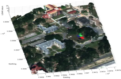
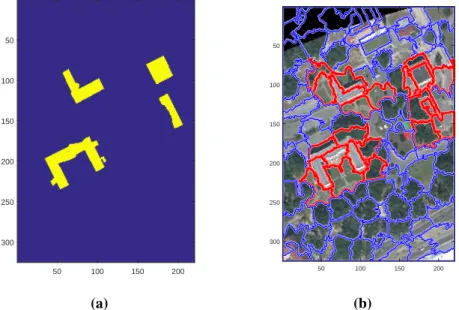
test on sub-image 3. . . 120 6.39 Four LiDAR lines in MUUFL Gulfport data, shown in Google Earth. . . 121 6.40 RGB image of MUUFL Gulfport data. . . 121 6.41 Scatterplot of LiDAR line 1 point cloud in MUUFL Gulfport campus 1 data. 122 6.42 Raster image of the first return MUUFL Gulfport LiDAR data. . . 122 6.43 Open Street Map imagery over MUUFL Gulfport campus 1. . . 123 6.44 The Ground Truth map and the SLIC segmentation map of the MUUFL
Gulfport HSI data for building detection. . . 124 6.45 The building signature for ACE detector and the ACE detection map for the
MUUFL Gulfport HSI data. . . 124 6.46 The histogram and peaks of the LiDAR values of building points. . . 125 6.47 The LiDAR confidence maps for building detection in the MUUFL
Gulf-port HSI data. . . 125 6.48 The fusion test confidence maps for building detection in the MUUFL
Gulf-port HSI data for SVM and min methods. Train on campus 1 and test on campus 2. . . 126 6.49 The fusion test confidence maps for building detection in the MUUFL
Gulf-port HSI data for taking the max and mean of the sources. Train on campus 1 and test on campus 2. . . 126 6.50 The fusion test confidence maps for building detection in the MUUFL
6.51 The fusion test confidence maps for building detection in the MUUFL Gulf-port HSI data for the proposed MICI and MR-MICI methods. Train on campus 1 and test on campus 2. . . 127 6.52 The Overall ROC curve for building detection for MUUFL Gulfport data. . 128 6.53 The difference map in the MUUFL Gulfport HSI data between LiDAR
points picked by MR-MICI and mean of the LiDAR points versus rasterized LiDAR imagery. . . 129 6.54 The difference map in the MUUFL Gulfport HSI data between min and
max of the LiDAR points and rasterized LiDAR imagery. . . 129 6.55 The ROC curve for building detection for MUUFL Gulfport data, scored
on the difference map between LiDAR edge map and mean maps. Train on Campus 1, test on Campus 2. . . 130 6.56 The ROC curve for building detection for MUUFL Gulfport data, scored
on the difference map between min and max maps. Train on Campus 1, test on Campus 2. . . 130 6.57 The ROC curve for building detection for MUUFL Gulfport data, scored
on the difference map between LiDAR edge map and mean maps. Train on Campus 2, test on Campus 1. . . 131 6.58 The ROC curve for building detection for MUUFL Gulfport data, scored
on the difference map between min and max maps. Train on Campus 2, test on Campus 1. . . 131 6.59 The Ground Truth map and the SLIC segmentation map of the MUUFL
6.60 The Ground Truth map and the SLIC segmentation map of the MUUFL
Gulfport HSI data for road detection. . . 132
6.61 The fusion test confidence maps for building detection in the MUUFL Gulf-port HSI data for the proposed MICI and MR-MICI methods. Train on campus 1 and test on campus 2. . . 133
6.62 The Overall ROC curve for sidewalk detection for MUUFL Gulfport data. . 133
6.63 The Overall ROC curve for road detection for MUUFL Gulfport data. . . . 134
6.64 The RGB image of weed in the soybean-weed data. . . 134
6.65 The height map of the soybean-weed data. . . 134
6.66 The L-band image of the soybean-weed data. . . 134
6.67 The B-band image of the soybean-weed data. . . 135
6.68 The Gabor filtered image of the soybean-weed data height map. . . 135
6.69 The Ground Truth map of weed in the soybean-weed data. . . 135
6.70 The SLIC segmentation map of the soybean-weed data. . . 135
6.71 The ROC curve for weed detection in the soybean-weed data. . . 136
6.72 The confidence map obtained from MICI fusion for the soybean-weed data. 136 6.73 The confidence map obtained from the MR-MICI fusion for the soybean-weed data. . . 136
6.74 Contamination data set for MICI Regression model experiments. . . 138
6.75 The relationship between the Gaussian kernel width and RVM RMSE. . . . 142
6.76 The relationship between the Gaussian kernel width and Aggregate MIR RMSE. . . 143
6.78 Comparison of ROC curve performance using top-down initialization and bottom-up initialization. . . 153 6.79 Comparison of the two optimization schemes: sampling by measure
ele-ment or sampling according to the valid intervals. . . 154 6.80 An illustration for the subset and superset relationships between binary
fuzzy measure elements given four sources. . . 155 6.81 Relationship of fitness values vs. number of iterations for MICI binary
LIST OF ABBREVIATIONS AND ACRONYMS
AHI Advanced Himawari Imager
BFM binary fuzzy measure
CI Choquet integral
DD Diverse Density
DEM dital elevation model
DSM digital surface model
EM Expectation-Maximization
EMI electro-magnetic induction (sensor)
FAR false alarm rate
GA genetic algorithm
GIS geographic information systems
GPR ground penetrating radar
GPS Global Positioning System
GSD ground sample distance
HSI hyperspectral image
IR infrared (sensor)
kNN K-nearest neighbor
LiDAR or LIDAR Light Detection and Ranging LCFI linguistic Choquet fuzzy integral
MIL Multiple Instance Learning
MILES Multiple-Instance Learning via Embedded Instance Selection MIR Multiple Instance (Multiple) Regression
MKL Multiple Kernel Learning
MR-MICI Multi-Resolution Multiple Instance Choquet Integral
MS multispectral (imagery)
PAN panchromatic (imagery)
PSO particle swarm optimization
RFC-MIR Robust Fuzzy Clustering Multiple Instance Regression ROC receiver operating characteristic (curve)
SAR synthetic aperture radar
LIST OF SYMBOLS AND NOTATIONS
g A fuzzy measure B Total number of bags
m Total number of sources (e.g. classifiers) to be fused N Total number of data points
Nh Total number of source combinations in multiresolution fusion
Cg(·) The Choquet integral output on an input computed with fuzzy measureg
P Measure population size in the evolutionary algorithm I Maximum number of iterations in the evolutionary algorithm F0
P Fitness values for all measures in the initial population in the evolutionary algorithm Ft
P Fitness values for all measures in Iterationt
F∗ Best (highest) current fitness value
g∗ Best current measure with the highest fitness value
G All measures in the current measure population
G{p} Thepthmeasure in measure populationG η Rate of small-scale mutation
ABSTRACT
Imagine you are traveling to Columbia, MO for the first time. On your flight to Columbia, the woman sitting next to you recommended a bakery by a large park with a big yellow um-brella outside. After you land, you need directions to the hotel from the airport. Suppose you are driving a rental car, you will need to park your car at a parking lot or a parking struc-ture. After a good night’s sleep in the hotel, you may decide to go for a run in the morning on the closest trail and stop by that recommended bakery under a big yellow umbrella. It would be helpful in the course of completing all these tasks to accurately distinguish the proper car route and walking trail, find a parking lot, and pinpoint the yellow umbrella.
Satellite imagery and other geo-tagged data such as Open Street Maps provide effective information for this goal. Open Street Maps can provide road information and suggest bakery within a five-mile radius. The yellow umbrella is a distinctive color and, perhaps, is made of a distinctive material that can be identified from a hyperspectral camera. Open Street Maps polygons are tagged with information such as “parking lot” and “sidewalk.” All these information can and should be fused to help identify and offer better guidance on the tasks you are completing.
Supervised learning methods generally require precise labels for each training data point. It is hard (and probably at an extra cost) to manually go through and label each pixel in the training imagery. GPS coordinates cannot always be fully trusted as a GPS device may only be accurate to the level of several pixels. In many cases, it is practically infeasible to obtain accurate pixel-level training labels to perform fusion for all the imagery and maps available.
a 3D point cloud. The imagery may have different resolutions, scales and, even, coordi-nate systems. Previous fusion methods are generally only limited to data mapped to the same pixel grid, with accurate labels. Furthermore, most fusion methods are restricted to only two sources, even if certain methods, such as pan-sharpening, can deal with different geo-spatial types or data of different resolution. It is, therefore, necessary and important, to come up with a way to perform fusion on multiple sources of imagery and map data, possibly with different resolutions and of different geo-spatial types with consideration of uncertain labels.
I propose a Multiple Instance Choquet Integral framework for resolution multi-sensor fusion with uncertain training labels. The Multiple Instance Choquet Integral (MICI) framework addresses uncertain training labels and performs both classification and regres-sion. Three classifier fusion models, i.e. the noisy-or, min-max, and generalized-mean models, are derived under MICI. The Multi-Resolution Multiple Instance Choquet Integral (MR-MICI) framework is built upon the MICI framework and further addresses multi-resolution in the fusion sources in addition to the uncertainty in training labels. For both MICI and MR-MICI, a monotonic normalized fuzzy measure is learned to be used with the Choquet integral to perform two-class classifier fusion given bag-level training labels. An optimization scheme based on the evolutionary algorithm is used to optimize the models proposed. For regression problems where the desired prediction is real-valued, the primary-instance assumption is adopted.
The algorithms are applied to target detection, regression and scene understanding ap-plications. Experiments are conducted on the fusion of remote sensing data (hyperspectral and LiDAR) over the campus of University of Southern Mississippi - Gulfpark.
Cloth-clusion and the proposed algorithms can successfully detect the targets in the scene. A semi-supervised approach is developed to automatically generate training labels based on data from Google Maps, Google Earth and Open Street Map. Based on such training la-bels with uncertainty, the proposed algorithms can also identify materials on campus for scene understanding, such as road, buildings, sidewalks, etc. In addition, the algorithms are used for weed detection and real-valued crop yield prediction experiments based on remote sensing data that can provide information for agricultural applications.
Chapter 1
Introduction
Multi-sensor fusion methods aim to combine and integrate information obtained from mul-tiple sensor sources while reducing uncertainties in the data and providing more detailed information [1,2]. Each of the sensor sources may provide complementary and reinforcing information that is helpful in applications such as target detection, classification, or scene understanding [3]. Take remote sensing applications for example, imagery can be obtained from multiple sensors such as hyperspectral and LiDAR (light detection and ranging). Hy-perspectral imaging sensors can provide spectral information about materials in the scene across a wide range of wavelengths while LiDAR data can provide height information. If a road and a building rooftop are built with the same material (say, asphalt), hyperspectral information alone may not be sufficient to tell them apart. However, LiDAR data provides height information and can easily distinguish the two. On the other hand, a highway and a biking trail can be at the same elevation and using LiDAR data alone may not be
suf-be primarily asphalt, and a biking trail, which is likely to suf-be covered in dirt. It would suf-be, thus, valuable to take advantange and fuse the information provided by multiple sensors in order to produce more detailed information, such as a better classification result or a more comprehensive understanding of the scene [2,4–6].
The Choquet integral (CI) has a long history of being an effective aggregation operator for non-linear fusion [3, 7–10]. A discrete Choquet integral integrates the input sources with respect to a fuzzy measure [11]. Compared with commonly used aggregation oper-ators such as weighted arithmetic means [12], the Choquet integral is able to model the relationship amongst the combinations of the sources and can flexibly represent a wide variety of aggregation operators [7, 13]. In this dissertation, the monotonic normalized discrete Choquet integral [14] is used as the aggregation operator for sensor fusion.
The standard Choquet integral fusion method assumes that (1) the data to be fused are homogeneous (of the same data type and with the same resolution) and (2) there are training labels available for each data point. It is generally assumed that the data provided by multiple sources for fusion must be of the same type, of the same resolution, on the same grid, or be possible to match and link individual data points together if the data types are arbitrary/heterogeneous [15]. That is to say, the standard CI fusion method requires data from mdifferent sensors produce data that has a one-to-one correspondence, or that some form of pre-processing is needed to transform all sources to the same resolution and perform matching. In addition, the data has to be on the same grid or scale, so pixel(i, j) in sensor image data 1 should correspond to pixel (i, j) in sensor image data m exactly. The image data valuesXk
ij,k = {1, ..., m}as well as its classification or regression labels
lij are also assumed to be known for each training pixel/data point in the image [16]. This assumption raises two problems. First, the assumption about homogeneous data
source types does not generally hold in real applications for sensor fusion. Existing op-tical sensors operate on varying spatial and spectral and temporal resolutions [17] and it is not necessarily feasible to convert all data to the same resolution or map to the same grid. Techniques such as rasterization and image registration [18, 19] have been proposed to perform co-registration of heterogeneous geospatial information sources. However, ras-terized images may lose some of its original information. Suppose a hyperspectral imaging (HSI) camera scans the scene and provides an image with1-meter ground sample distance (GSD) [20]. That means each pixel in the hyperspectral image covers 1×1m2 area. Li-DAR technology, on the other hand, produces point clouds by densely sample the surface of the earth in the scene. There can be several LiDAR data points inside an1×1m2 area. One way to rasterize LiDAR data is by projecting the LiDAR data points into the pixel coordinate plane of the HSI image [21] and obtain one single LiDAR value (Z coordinate value, usually height information) for each pixel. Then, data fusion between the HSI and rasterized LiDAR data can be performed pixel-by-pixel on the image grid. However, the dense LiDAR point cloud data can offer higher geographic accuracy [22] as the data does not depend on grid size. Each LiDAR data point provides a certain degree of information and it would be nice to take all available information into account. Besides, most image registration methods rely heavily on both the accuracy of input images and registration pa-rameters [18, 23] and can also bring in another layer of uncertainty regarding geometric misalignment and mismatch [15,21].
Second, even assuming that homogeneous data is available for fusion or that there is a noiseless way to transform heterogeneous data, standard supervised learning methods require accurate labels for each training data point. However, data-point specific labels
remote sensing applications, for example, some Global Positioning System (GPS) device may only be accurate to the level of several meters [24]. Depending on the GSD of the imagery, the target ground truth locations in the scene measured by a GPS can only be accurate to the level of several pixels. It is, thus, difficult to pinpoint accurate pixel-level target locations and provide accurate training labels.
To address these two problems, this dissertation proposes a Multiple Instance Choquet Integral (MICI) framework for both multi-sensor classifier fusion and regression that can deal with uncertainty in training labels. Three variations of the objective functions based on three models, i.e. noisy-or, min-max and generalized-mean models, were derived for the MICI classifier fusion framework. A monotonic normalized fuzzy measure is learned to be used with the Choquet integral to perform two-classs classifier fusion given bag-level train-ing labels. An optimization scheme ustrain-ing an evolutionary algorithm is used to optimize the models proposed. For regression problems where the desired prediction is real-valued, this dissertation adopts the “primary-instance” assumption that there is one primary instance re-sponsible for the label for each bag [25] and proposes a Multiple Instance Choquet Integral Regression model that can fuse multiple sources with real-valued label as well as taking into account the uncertainties in the label.
Furthermore, this dissertation proposes a Multi-Resolution Multiple Instance Choquet Integral (MR-MICI) framework that takes in heterogeneous data (for example, images at different resolutions or data of different geospatial types) from multiple sensors with un-certainty in training labels and perform fusion. The proposed MR-MICI algorithm works under the assumption that at least one point in each bag from each data source is accurate but the remaining data points in the bags can have uncertain labels. The proposed MR-MICI algorithm also learns a monotonic normalized fuzzy measure to be used with the
Choquet integral to perform fusion on heterogeneous data sources.
Experiments were conducted based on the proposed algorithms on both synthetic data and real applications such as target detection and scene understanding in remote sensing imagery. Results indicate that the proposed MICI framework can successfully learn a set of fuzzy measure to be used with the Choquet integral to effectively perform classifier fusion and regression while dealing with uncertainties in training labels. Results also indi-cate that the proposed MR-MICI framework can successfully perform classifier fusion and yield better classification accuracy on heterogeneous data (multi-resolution data and data of different geospatial types such as HSI and LiDAR) while taking into account uncertain labels.
Chapter 2
Literature Review
This chapter provides a literature review on Multiple Instance Learning frameworks in-cluding MIL classification and MIL regression. This chapter also provides definitions for fuzzy measures and the Choquet integral and reviews previous methods in learning a fuzzy measure. This chapter also reviews the existing literature in sensor fusion, especially fu-sion with the Choquet integral and fufu-sion of heterogeneous data types and multiresolution fusion.
2.1
Multiple Instance Classification
The Multiple Instance Learning (MIL) framework was first proposed in [26] to address uncertainty and inaccuracy in labeled data in supervised learning. In the MIL framework, training labels are associated with sets of data points (“bags”) instead of each data point (“instance”). In the scenario of two-class classification, the standard MIL assumes that a bag is labeled positive if at least one instance in the bag is positive and a bag is labeled
negative if all the instances in the bag are negative. Figure 2.1 shows the illustration of MIL bags. Assuming the red-colored points are positive instances and blue-colored points are negative instances. The two bags on the top row are, therefore, negative bags, as all the instances in the bags are negative. The three bags on the bottom row are positive bags, as there is at least one positive instance in the bags. A more generalized view of the MIL was also introduced in the literature [27]. The generalized MIL does not follow the restriction of the standard MIL assumption [28, 29]. The standard MIL assumes that a bag’s label depends on the labels of the instances in the bag, while the generalized MIL assumes that a bag’s label depends on the “interaction” between instances in the bag [28, 29]. In this dissertation, only the standard MIL assumption is discussed as it fits the task of sensor fusion at hand.
Negative Bags
Positive Bags
Figure 2.1: Illustration of bags in multiple instance learning. Red color marks positive
instances and blue color marks negative instances. The two bags on the top row are negative bags and the three bags on the bottom row are positive bags.
Figure 2.2 illustrates the differences between standard supervised classification, multi-ple instance learning classification and embedded multimulti-ple instance learning classification
ciated class label (such as marked in orange or blue color in Figure 2.2) [30]. The instance-space paradigm classifies instances based on their values at the instance level and draws a decision boundary between classes. The bag-space paradigm discriminates information at the bag-level. Distances between bags are computed and a standard distance-based clas-sifier may be applied such as the K-nearest neighbor (KNN) classifier [30, 31]. In the embedded-space paradigm, each bag is often mapped into a high-dimensional space. Each feature vector in the high-dimensional space for each bag represents information from the entire bag and all the instances in the bag. A discriminative classifier is then applied to the feature vectors in the embedded space; thus classifying entire bags. Selected notable MIL classification methods are discussed in detail as follows.
Standard Classification Multiple Instance Learning Embedded Multiple Instance Learning
Figure 2.2: Illustration of standard supervised classification, multiple instance learning
classification and embedded multiple instance learning classification. The left column is training stage and the right column is testing stage. Orange color marks positive instances/bags and blue color marks negative instances/bags in the feature space.
The EM-DD technique [32] combines the Expectation-Maximization (EM) method [33] and the Diverse Density (DD) approach [13, 26, 34]. For two-class classification problems, the maximum Diverse Density is defined as [13,34]:
arg max x Y i P r(x=t|Bi+)Y i P r(x=t|Bi−), (2.1)
whereBi+is theithpositive bag andB−
i is theithnegative bag,Bij is the individual feature values of thejth instance of theith positive bag,t is the true concept, andxrepresents all the points in feature space. Maron et al. [34] proposed a noisy-or model, where for all the instances in each bag,
Y i P r(x=t|Bi+) = 1−Y j 1−P r(x=t|Bij+), (2.2) and Y i P r(x=t|Bi−) =Y j 1−P r(x=t|Bij−). (2.3)
The causal probability of an individual instance on a potential target was computed based on the distance between them using
P r(x=t|Bij) = exp(− kBij−xk2), (2.4)
whereBij is the individual feature values of thejthinstance of theithbag.
To extend the DD model, the EM-DD views the relationship between all the instances in the bag and the label of the bag (which instance corresponds to the label of the bag?) as a latent variable that can be estimated using the EM approach [32]. In the E-step, one instance is picked from each bag as the most influential instance for its bag-level label. In the M-step, the DD is maximized by a gradient ascent search and the process is iterated
may pick, but the convergence rate is undetermined [32]. EM-DD scales up well as the bag size increases but the performance will depend on initialization. The EM-DD algorithm can be used for both MI classification and regression [32].
Citation-kNN [35] algorithm uses the Hausdorff distance to compute distance between two bags and assigns bag-level label based on the K Nearest Neighbor rules [36]. The Hausdorff distance for two BagsAandB is defined as:
H(A, B) = max{h(A, B), h(B, A)}, (2.5)
and
h(A, B) = max
a∈A minb∈B ka−bk, (2.6)
whereaandbare instances in bagsAandB, respectively. A modified version of Hausdorff distance can be computed as follows instead of (2.7):
h(A, B) =kath∈Amin
b∈B ka−bk. (2.7)
Citation-kNN algorithm then assigns label for bagBi considering its K nearest neighbors (“references”) and alsoC bags that countsBi as a neighbor (“citers”). The Citation-kNN algorithm extends the traditionalKNearest Neighbor to suit multiple instance learning pur-poses. Extensions of citation-kNN include Bayesian citation-kNN [37] and fuzzy citation-kNN [38,39].
Andrews et al. [40] proposed two MIL formulations, mi-SVM and MI-SVM, based on support vector machine (SVM) learning approaches. For the mi-SVM two-class classifica-tion problem, the objective funcclassifica-tion is defined as [40]:
min {yi} min w,b,ξ 1 2kwk 2 +CX i ξi, (2.8)
such that
X
i∈I
yi+ 1
2 ≥1,∀i:yi(<w,xi >+b)≥1−ξi, ξi ≥0 (2.9) wherewis the weights,bis the bias,yiis the instance-level label,ξiare the slack variables (similar to that of a standard SVM). The labels Y satisfy the MIL assumption. The mi-SVM algorithm learns a linear discriminate function and maximizes the margin to separate the positive from the negative classes based on instance labels. MI-SVM extends based on mi-SVM and defines the objective function as [40]:
min w,b,ξ 1 2kwk 2 +CX I ξI, (2.10) such that ∀I :YImax i∈I (<w,xi >+b)≥1−ξI, ξI ≥0, (2.11) where YI is the label for bagI. The MI-SVM objective function extends the concept of margin maximization to the bag-level.
Multiple-Instance Learning via Embedded Instance Selection (MILES) is a represen-tative embedded multiple instance learning method [41, 42]. MILES maps both training and testing bag into high-dimensional feature vectors and then performs classification in the mapping space using a one-norm SVM [43]. The distance between an instancexkand a bagBi is computed as the smallest distance betweenxk and all the instances in bag Bi [41,43]: s xk |Bi = max j exp − xij −xk 2 σ2 ! , (2.12)
wherexk is the feature vector forkth instance,Bi is theithbag, xij is thejthpixel in the
ithbag, andσis a fixed parameter. The feature vector for bagB
In this way, a high-dimensional feature vector is constructed based on the distance values. The dimensionality of the feature vector is equal to the number of instances in a data set. The feature vector reflects the similarity between each instance in the data set and each bag. The complete feature mapping mgiven alll+ positive and l−
negative bags is written as [41,43]: [m+1, . . . ,m+l+,m − 1, . . . ,m − l−]T = [m(B+1), . . . ,m(B+l+),m(B − 1), . . . ,m(B − l−)] T = s(x1,B+1) . . . s(x1,B+l+) s(x1,B − 1) . . . s(x1,B − l−) s(x2,B+1) . . . s(x2,B+l+) s(x2,B − 1) . . . s(x2,B − l−) .. . ... ... ... ... ... s(xn,B+ 1) . . . s(xn,B + l+) s(xn,B − 1) . . . s(xn,B − l−) T , (2.13)
where the complete mapping for all the bags to all the training instances has dimensionality N umBags×N umInstances.
After feature mapping, a one-norm Support Vector Machine (SVM) is used to perform classification and simultaneously select the most discriminating training instances. The one-norm SVM classifier can be expressed as follows:
y =sign n X k=1 wks(xk,Bi) +b ! , (2.14)
where weights w = [w1, w2, . . . , wk, . . . , wn]T (k = 1, . . . , n for n training instances) and bias b are model parameters. The weights w and bias b are determined through the following optimization problem:
min w,b,η,ξλ n X k=1 |wk|+c1 l+ X i=1 ξi+c2 l− X j=1 ηj (2.15) with constraints wTm+i +b +ξi > 1; − wTm−j +b +ηj > 1; ξi, ηj > 0 for i =
1, ..., l+ andj = 1, ..., l−. In the above formulation,l+ andl−are the number of positive bags and negative bags, respectively. m+i is the mapping for all positive bags andm−i is the mapping for all negative bags. ξ and η are hinge loss parameters that are estimated through the above linear programming problem together with the weightswand biasb. λ, c1andc2 are scale parameters set by the user. These parameters must satisfy the following
constraints: c2 = 1 − c1 and 0 < c1 < 1. These constraints ensure the total training
error (i.e., the objective function measure we are trying to minimize through optimization) is associated with a convex combination of training error on both the positive bags and negative bags [41].
After the training, the instances corresponding to non-zero weights,w, are identified as the “selected” and “discriminative” training samples. These samples will be used during the feature mapping and classification of test data. The usage of the one-norm penalty on the weights is to promote sparsity and drive more elements ofwto zero, thus making the testing process efficient.
Inspired by drug activity prediction problem [26], Multiple Instance Classification has wide applications in natural scene classification [44, 45], human action recognition in videos [46], object detection and tracking [47–49], context identification and context-dependent learning [43,50], and music information retrieval [51,52].
2.2
Multiple Instance Regression
Multiple instance regression (MIR) deals with multiple instance problems where the pre-diction values are real-valued instead of class labels. MIR has been used in the literature
compatibility complex class II (MHC-II) molecules [53], predicting aerosol optical depth from remote sensing data [54,55], and predicting crop yield [55–57].
Ray and Page [25] first proposed an MIR algorithm based on the “primary-instance” assumption, which assumes there is one primary instance in a bag that is responsible for the real-valued bag-level label. A linear regression hypothesis was assumed and the goal is to find a hyperplaneY =Xbsuch that
b= arg min b n X i=1 L(yi, Xip,b), (2.16)
where Xip is the primary instance in bag i, and L is some error function. An Expecta-tion MaximizaExpecta-tion (EM) algorithm was proposed to solve for the ideal hyperplane. First, a random hyperplane was used for initialization. For each instance j in each bag i, the errorLof the instance Xij to the hyperplaneY = Xbwas computed asL(yi, Xij,b) =
(yi−Xijb)
2
. In the E step, the instance with the lowest errorLwas selected as the “pri-mary instance.” In the M step, a new hyperplane was constructed by performing a multiple regression over all the instances selected in the E step. The two steps were repeated until the algorithm converges and the best hyperplane solution was returned. Their algorithm was tested using synthetic data sets only but showed benefits of multiple instance regres-sion over ordinary regresregres-sion, especially when the non-primary instances in the bag were not correlated with the primary instances.
Dooly et al. [58] presented three multiple-instance variants of k-Nearest Neighbor (k-NN) [59], citation-kNN [35] and the diverse density algorithms [34] for real-valued prediction. The minimal Hausdorff distance from [35] was used to measure the distance between two bags. Given two sets of pointsA=a1, ...amandB =b1, ..., bn, the Hausdorff
distance is defined as:
H(A, B) = max{h(A, B), h(B, A)}, (2.17)
where h(A, B) = maxa∈Aminb∈Bka−bk, ka−bk is the Euclidean distance between points a and b. The Hausdorff distance, however, is very sensitive to outliers. If there is one point in B that is in some very large distance from all points in A, the Hausdorff distance will depend entirely on this one outlier point.
In their MI k-NN algorithm, the prediction made for a bagB is the average label of the k closest bags (measured in Hausdorff metric). In their MI citaion-kNN algorithm, the prediction made for a bag B is the average label of the R closest bag neighbors of B(measured in Hausdorff metric) andC-nearest citers, where the “citers” include the bags whereBis a one of theirC-nearest neighbors. It is generally recommended thatC =R+2. The third variant, a diverse density approach for the real-valued setting, maximizes
b Y i=1 P r(r|Bi) (2.18) where P r(t|Bi) = (1− |li−Label(Bi|t)|)/Z, (2.19)
b is the total number of bags, t is the target point, li is the label for the ith bag, and Z is a normalization constant. Their results showed good performance of all three variants on a benchmark Musk Molecules data set [26, 58] but the performance of both the near-est neighbor and diverse density algorithms are very sensitive to the number of relevant features, as expected based on the sensitivity of the Hausdorff distance.
with each point and used the Hausdorff metric as well to help classify a bag as positive (if the points in the bag are within some Hausdorff distance from target concept points). Their algorithm differs from the supervised MIR in that the standard supervised MIR learns from a given set of training bags and bag-level training labels, while [60] applies an online agnostic model [61–63] where the learners make predictions as the bagxt is presented at iteration t. [64] also used the idea of online MIR, i.e. use the latest arrived bag with its training label to update the current predictive model. This work is also extended in [65].
Cheung and Kwok [66] proposed a regularization framework for MIR by defining a loss function that takes into consideration both training bags and training instances. The first part computes the error (loss) between training bags label and its predictions and the second part considers the loss between the bag label prediction and all the instances in the bag. Cheung and Kwok still adopted the “primary instance” assumption but simplified to assume the primary instance was the instance with the highest prediction output value. Their model provided comparable or better performance on the Musk Molecules data set [58] as citation-kNN [35] and Multiple Instance kernel-based SVM [66,67].
Most MIR works methods discussed thus far only provided theoretical discussions or results on synthetic data set(s). Wagstaff et al. in [56, 57] started to further investigate more applications of MIR to predict crop yield from a remote sensing data set collected over California and Kansas. [56] provided a novel method for inferring the “salience” of each instance with regard to the real-valued bag label. The salience of each instance, i.e. its “relevance” with respect to all other instances in the bag to predict the bag label, is the weight associated with each instance. The salience values were defined to be non-negative and sum to one for all instances in each bag. Like Ray and Page [25], Wagstaff et al. followed the “primary-instance” assumption but their primary instance, or “exemplar” of a
bag, is the weighted average of all the points in the bag instead of one single instance from the bag. Given training bags and instances, a set of salience values are solved based on a fixed linear regression model and given the estimated salience, the regressor is updated and the algorithm reiterates until convergence. This work did not intend to provide predictions over new data but instead focused on understanding the contents (the salience) of each training instance.
Wagstaff et al. then made use of the salience learned to provide predictions for new, un-labeled bags by proposing an MI-ClusterRegress algorithm (or in some references, Cluster-MIR algorithm) that mapped instances onto (hidden) cluster labels [57]. The main assump-tion of MI-ClusterRegress is that the instances from a bag are drawn (with noise) from a set of underlying clusters and one of the cluster is “relevant” to the bag-level labels. After ob-tainingkclusters for each bag by EM (Expectation Maximization)-based Gaussian mixture models (or any other clustering method), a local regression model is constructed for each cluster. MI-RegressCluster then selects the best-fit model and use it to predict labels for test bags. A support vector regression learner [68] is used for regression prediction. Results on simulated and predicting crop yield data sets show that modeling the bag structure when the structure (cluster) is present is effective for regression prediction, especially when the cluster numberkis equal to or larger than what is actually present in the bags.
More recently, Trabelsi and Frigui [69] proposed the Robust Fuzzy Clustering for MIR (RFC-MIR) algorithm that, similar to Cluster-MIR, clusters the training instances and learns multiple regression models for each cluster. RFC-MIR uses fuzzy clustering meth-ods such as the fuzzy c-means (FCM) [70] or possibilistic c-means (PCM) [70], and uses features as well as labels in clustering. The current regression model was assumed to be
bag. Results on synthetic and predicting crop yield data sets show improved accuracy. Both Cluster-MIR and RFC-MIR combine all instances from all training bags for clustering.
MIR has since then been used in more real-world applications. EL-Manzalawy et al. [53] adapted the 1-norm SVM classifier in the MILES algorithm [41] to a support vector regression (SVR) model and applied their MHCMIR method to predict MHC-II binding affinity in molecules to help develop new vaccine. Pappas and Popescu-Belis [71] extends the works of Wagstaff et al. to deal with high dimensions and learns the instance relevance together with the target labels with application in aspect-based sentiment rating and analy-sis using texts from datasets such as TED talks or audiobooks. Hsu et al. [72] proposed the Augmented MIR (AMIR) algorithm to estimate object contours from images. The bound-ing box outside of an object in the image is regarded as “bags” and the object contour pixels are the instances. The gradient descent optimization method was used to solve for the weights of the regressor. The AMIR algorithm was evaluated using the Pascal VOC 2007 Segmentation Challenge data set and obtained good results in semantic segmenta-tion. Notably, Wang et al. [54,55] proposed a novel, probabilistic and generalized mixture model for MIR based on the primary-instance assumption. It is assumed that the bag label is a noisy function of the primary instance, and the conditional probabilityp(yi|Bagi)for predicting labelyi for theith bag is dependent entirely on the primary instance. A binary random variable zij is defined such that zij = 1 if the jth instance in the ith bag is the primary instance andzij = 0if otherwise. The mixture model for each bagiis written as:
p(yi|bagi) = bi X j=1 p(zij = 1|bagi)p(yi|xij) (2.20) = bi X j=1 πijp(yi|xij), (2.21)
p(yi|xij)is the label probability given the primary instancexij andbi is the total number of instances in the ith bag. Therefore, the learning problem is transformed to learning the mixture weights πij and p(yi|xij)from training data and an EM algorithm is used to optimize the parameters. This work discussed several methods to set the priorπij, including using deterministic function, or as a (Gaussian) function of prediction deviation, or as a parametric function (in this case a feedforward neural network). It was discussed in [55] that several previous algorithms, including Prime-MIR [25] and Pruning-MIR [54], are in fact the special case of the mixture model they proposed. Their results showed better performance on simulated data as well as for predicting aerosol optical depth (AOD) from remote sensing data and predicting crop yield applications, compared with the Cluster-MIR [57] and Prime-MIR [25] algorithms described above.
Overall, the study of Multiple Instance Regression has been in the literature for about one and a half decades and most studies base their algorithms on the primary-instance assumption proposed by Ray and Page in 2001. Linear regression was used in most cases if a regressor was used and experiments have been conducted on synthetic data sets as well as real data sets such as crop yield and AOD prediction.
2.3
Fuzzy Measure and Choquet Integral
The Choquet integral (CI) has a long history of providing an effective framework for non-linear information fusion [8, 9, 73–75]. The CI is an aggregation operator based on the fuzzy measures [11]. Depending on the values of each element in the fuzzy measure, the CI can represent a variety of relationships and combinations amongst the information sources.
fuzzy measures for the CI [76,77]. This section provides description and definition of the fuzzy measure and the Choquet integral and reviews previous methods in learning the fuzzy measures, specifically within the CI.
2.3.1
Fuzzy Measure
Consider the case that there are m sources, C = {c1, c2, . . . , cm}, for fusion. The setC contains2m −1 non-empty subsets. The power set of all (crisp) subsets ofC is denoted 2C.
Definition 2.3.1. A monotonic and normalizedfuzzy measure,g, is a real valued function that maps2C →[0,1]. It satisfies the following properties [14,78–80]:
1. g(∅) = 0;
2. g(C) = 1;normalized
3. g(A)≤g(B)ifA⊆B andA, B ⊆C. monotonic
One special and useful case of the fuzzy measure is the Sugeno λ-measure [9, 11,
81, 82]. The Sugeno λ-measure is defined as follows and will be further referred to in Section 2.3.3.
Definition 2.3.2. ASugenoλ-measure,g, is a real valued function that maps2C →[0,1]. Letλ ∈(−1,+∞), it satisfies the following properties [9,11,81,82]:
1. g(C) = 1;normalized
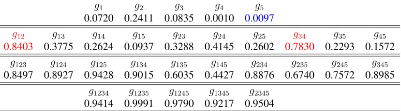
2. ifA, B ⊆C andA∩B =∅, theng(A∪B) = g(A) +g(B) +λg(A)g(B). Fuzzy measures, in general, model the relationship amongst the sources. Each measure element value represents the power/“worth” of a certain combination of the sources. In this dissertation, the measure elements within a fuzzy measure are denoted with a subscript
matching its corresponding subset. For example, element g1 corresponds to subset {c1},
elementg12corresponds to subset{c1, c2}, etc. Note thatghas a total of2m −1elements
andg123...m is always equal to 1 (property2). All other measure elements hold real values between[0,1]and satisfy monotonicity (property3). Non-monotonic fuzzy measures have been studied in the literature [82–84] but this dissertation only deals with monotonic and normalized fuzzy measures. The term “fuzzy measures” in this dissertation always refers to monotonic and normalized fuzzy measures.
Figure 2.3 shows an illustration of the monotonicity property in between fuzzy mea-sure elements given four sources. Take meamea-sure element g23 for example, g2 and g3 are
its subsets andg123 andg234 are its supersets. Therefore, the element value ofg23satisfies
g23 ≥ g2, g23 ≥ g3, g23 ≤ g123 and g23 ≤ g234. The red arrows show one path to “climb
up the lattice” of the fuzzy measure elements. Notice that the measure element that cor-responds to the full set, g1234 in this case, is always equal to 1 (property 2). All measure
elements take values between zero and one.
g
1g
2g
3g
4g
12g
13g
14g
23g
24g
34g
123g
124g
134g
234g
1234Figure 2.3:An illustration for the subset and superset relationships between fuzzy
mea-sure elements given four sources. The red arrows describe one path for “climbing up the lattice”.
ing human evaluation and decision processes [87,88], image segmentation [89–91], image enhancement [92], gene ontology [93,94], medical diagnostic reasoning [95], and evaluat-ing the similarity between sets of levaluat-inguistic summaries [96].
2.3.2
Choquet Integral
Fuzzy measures are used to define fuzzy integrals such as the Sugeno fuzzy integral (here-inafter referred to as “the Sugeno integral”) [78] and the Choquet fuzzy integral (hereinafter referred to as “the Choquet integral”) [14, 97] in the literature. There has been studies on the statistical properties of the Choquet and Sugeno Integrals [98–100]. The Choquet inte-gral (CI) is a natural extension of the Lebesgue inteinte-gral [11,88] and has long been used as an effective aggregation operator [80].
Definition 2.3.3. The Choquet integral, denoted as (C)R, of a measurable function h with respect to fuzzy measuregis defined as [11,97]: (C)R
h dg=R∞
0 g({h > α})dα.
Note that if the functionh→[0,1], the∞sign will be replaced by1(integrating from 0 to 1).
In this dissertation, the discrete Choquet integral is used to fuse information provided by different sources. Suppose the sources are the outputs from the set of m classifiers or regressors, C = {c1, c2, . . . , cm}, as mentioned above. Denote the classifier/regressor output ofkth classifier/regressor,ck, onnthdata point/instance,xn, ash(ck;xn).
Definition 2.3.4. Thediscrete Choquet integralon instancexngivenCis then computed as [10,11,80]: Cg(xn) = m X k=1 [h(ck;xn)−h(ck+1;xn)]g(Ak), (2.22)
whereCis sorted so thath(c1;xn)≥h(c2;xn)≥ · · · ≥h(cm;xn). Since there are onlym sources,h(cm+1;xn)is defined to be zero. The fuzzy measure element value corresponding to the subsetAk ={c1, . . . , ck}isg(Ak).
Gader et al. [3,101] applied the CI to multi-algorithm and multi-sensor fusion in land-mine detection applications. In their work, detectors were applied to Advanced Himawari Imager (AHI) hyperspectral and synthetic aperture radar (SAR) imagery or ground pen-etrating radar (GPR) and electro-magnetic induction (EMI) sensors and then, the CI was used to fuse the detector results. A linguistic version of the Choquet fuzzy integral (LCFI) was proposed in [102] and was used to perform fusion on GPR, EMI and infrared (IR) sensors also for landmine detection [103]. Liu et al. [104] used the CI to perform classifier fusion on Doppler radar sensor signals for fall detection in application towards elder care. Wang et al. [105] used the CI to integrate classifier results for Landsat image classification. The CI is and has provided effective fusion performance in fusing homogeneous possibility and probability distributions [106].
The Choquet integral has wide applications in pattern recognition [74] and classification [80, 107]. The Choquet integral has been applied with Multiple Kernel Learning (MKL) for pattern recognition and feature-level and decision-level fusion [108,109]. The CI was used in real applications such as landmine detection [9, 110], handwritten word recogni-tion [111, 112], text classification [113], gesture recognition [114], temperature prediction [115], chromosome abnormalities detection [116] and immunoinformatics [117]. The Cho-quet integral has also been used as a morphological image filter [80,118–120]. The discrete Choquet integral has also been proven to define a distance metric “with the versatility of
as aggregating aspect rating of restaurants from customer ratings [122].
2.3.3
Learning The Fuzzy Measure
In a classifier or regressor fusion problem with training data X = {x1,x2, . . . ,xN}, the
h(c1;xn), h(c2;xn), . . . , h(cm;xn)values for all n are known. The desired bag-level la-bels for sets of Cg(xn) values are known. A crucial aspect of using the CI to perform fusion is to learn all the element values of the fuzzy measureg from training data of this form [10]. This dissertation adopts and adapts the categorization in [80] and [123] and de-scribes below three main types of methods to learn the fuzzy measure, especially (but not necessarily limited) within the Choquet integral: least-square based approaches, gradient descent algorithm and evolutionary algorithms.
Least-square based approaches
As introduced in Section 2.3.1, forminput sources, there are2m−1non-empty subsets and hence2m−1fuzzy measure elements. Excludingg
123...m ≡1, there are2m−2unknown fuzzy measure element values to be estimated. A quadratic programming (QP) approach to solve for the fuzzy measures based on the least-square criteria was discussed in [11, 124]. Given the discrete CI formula in equation (6.10) and assuming the desired labels for the nth data point/instancexnisdn, the goal of the the least-square criteria is to find the fuzzy measuregso that the squared error is minimized between the Choquet integral outputs of all training data points givengand their desired labels [11,124]:
min g E 2 = N X n=1 (Cg(xn)−dn)2. (2.23)
given in Figure 2.3 in a bottom-up order:
g = [g1, g2, ..., gm, g12, g13, ..., g123...m−1, ..., g23...m] T
. (2.24)
DenoteΓmatrix as the difference matrix between the sources. Specifically, for each data point/instancen, the vectorΓnis defined to depict the differences between the sources [11]:
Γn= [0, ...,0, h(c1;xn)−h(c2;xn), ..., h(cm−1;xn)−h(cm;xn),0, ...,0]T . (2.25)
TheΓnhas onlym−1non-zero elements corresponding to the indices that occur in the CI definition in Eq. (6.10) [11].
Therefore, Eq. (2.23) can be rewritten as [11,80]: min g E 2 = N X n=1 (Cg(xn)−dn)2 (2.26) = N X n=1 ΓTn ·g+ [h(cm;xn)−dn] T ΓTn ·g+ [h(cm;xn)−dn] (2.27) = N X n=1 gTΓnΓTng+ 2 [h(cm;xn)−dn]ΓTng+ [h(cm;xn)−dn] 2 (2.28) =gT N X n=1 ΓnΓTn ! g+ 2 N X n=1 [h(cm;xn)−dn]ΓTn ! g + N X n=1 [h(cm;xn)−dn]2, (2.29)
We can then define, D ≡ N X n=1 ΓnΓTn ! , (2.30) Γ ≡ N X n=1 [h(cm;xn)−dn]Γn ! , (2.31) d2 ≡ N X n=1 [h(cm;xn)−dn]2, (2.32)
Hence, Eq. (2.29) can be written as min
g E
2 =gTDg+ΓTg+d2. (2.33)
Considering the monotonicity property of the fuzzy measureg(Section 2.3.1), we require: g1−g12≤0, g1−g13≤0, .. . g1−g123...m ≤0, .. . g123...m−1−g123...m≤0, .. . g23...m−g123...m ≤0, (2.34)
i.e., a total ofm(2m−1−1)inequality constraints on elements ofg. Notice thatg
123...m≡1
To write those inequality constraints inA·g+b≤0format, 1 0 · · · 0 −1 0 · · · 0 0 · · · 0 1 0 · · · 0 0 −1 · · · 0 0 · · · 0 .. . ... · · · ... ... ... · · · ... ... · · · ... 0 0 · · · 0 0 0 · · · 1 0 · · · 0 .. . ... · · · ... ... ... · · · ... ... · · · ... 0 0 · · · 0 0 0 · · · 0 0 · · · 1 (m(2m−1−1)×2m−2) · g1 .. . g12 g13 .. . g123...m−2 .. . g123...m−1 g134...m .. . g234...m ((2m−2)×1) + 0 .. . 0 0 .. . 0 .. . −1 −1 .. . −1 (m(2m−1−1)×1) ≤0 (2.35)
Note that the “-1” elements of thebvector comes from theg123...m≡1property.
Here is an example for three input sources (m = 3). We know there are a total of 9 constraints, i.e. g1 ≤g12, g1 ≤g13, g2 ≤g12, g2 ≤g23, g3 ≤g13, g3 ≤g23, g12 ≤g123 = 1, g13≤g123= 1, g23 ≤g123 = 1. (2.36)
The constraints can be rewritten in matrix form as: 1 0 0 −1 0 0 1 0 0 0 −1 0 0 1 0 −1 0 0 0 1 0 0 0 −1 0 0 1 0 −1 0 0 0 1 0 0 −1 0 0 0 1 0 0 0 0 0 0 1 0 0 0 0 0 0 1 (9×6) · g1 g2 g3 g12 g13 g23 (6×1) + 0 0 0 0 0 0 −1 −1 −1 (9×1) ≤0 (2.37)
Therefore, the problem of finding the fuzzy measuregaccording to the least square criteria formulated in Equation (2.33) turns into a quadratic programming (QP) problem [11,124]:
min
g E
2 =gTDg+ΓTg+d2,
subject toA·g+b≤0and0≤g ≤1.
(2.38)
The quadratic programming approach can then be solved by a QP solver such as the MAT-LAB built-inquadprog()function. This method is called “CI-QP” method and was used as a baseline comparison method later in the dissertation.
There are other approaches including a maximum split approach [125], a minimum variance method [126, 127] and a less constrained approach [128] as discussed in [123]. The maximum split approach models the pairs and interactions of the fuzzy measure ele-ments subject to the monotonicity and normalization constraints and solves the maximiza-tion problem using linear programming. The maximum split approach is a simple model [123] but introduces many variables and threshold parameters that must be chosen
care-fully [125]. The minimum variance method is based on a maximum entropy principle for fuzzy measures [127]. The principle argues that the maximum entropy capacities (fuzzy measures) “is the one that will exploit the most on average its arguments”, i.e. the opti-mal solution is the one that maximizes the entropy and hence minimizes the variance of the fuzzy measures (the link between the entropy and the variance can be seen in [127]). The less constrained approach [128] also writes the objective function based on the least squares criteria and optimizes the objective function subject to the properties of the fuzzy measure, using a convex quadratic program. However, it relaxes some of the constraints by converting the constraints on the fuzzy measures to constraints on the (unknown) over-all evaluation values. This methods can be regarded as a generalization of the standard least-squares QP method [123].
Gradient descent algorithm
A gradient-descent algorithm has been used to learn a fuzzy measure (a Sugenoλ-measure in this case) for the Choquet integral in [9]. The Sugeno λ-measure is defined in Sec-tion 2.3.1. Denote the measure element corresponding to a singleton set{cj}, also known as “densities”, asgj,j = 1, ..., m. Take the derivative of the Choquet integral in Equation (6.10), each partial derivative of Cg(xn)with respect to the measure element gj is given by: ∂Cg(xn) ∂gj = m X k=1 ∂g(Ak) ∂gj [h(ck;xn)−h(ck+1;xn)]. (2.39)
Recall the notation that fuzzy measure elementg(Ak)corresponds to the subsetAk =
-measure in Section 2.3.1,g(Ak)can be written as
g(Ak) = g({ck} ∪Ak−1)
=gk+g(Ak−1) +λgkg(Ak−1).
(2.40)
Then, the ∂g(Ak)
∂gj term in Equation (2.39) can be written as
∂g(Ak) ∂gj = ∂gk ∂gj + ∂g(Ak−1) ∂gj + ∂λ ∂gj gkg(Ak−1) +· · · +λ∂gk ∂gj g(Ak−1) +λgk ∂g(Ak−1) ∂gj . (2.41)
It is known in [11] that the valueλfor any Sugenoλ-measure satisfies (1 +λ) =
m Y
k=1
(1 +λgk), (2.42)
given the normalization property of the Sugeno λ-measure. Therefore, the ∂g∂λ
j term in
Equation (2.41), as proven in [9], can be rewritten as ∂λ ∂gj = λ 2+λ (1 +gjλ) h 1−(λ+ 1)Pm k=1 gk 1+gkλ i, λ6= 0. (2.43)
Then, a gradient descent algorithm can be used for any objective function (such as the aforementioned least-squares criterion) to solve for the fuzzy measure to be used with the Choquet integral [9,104].
Keller and Osborn proposed a neuron model and a “reward-punishment” training al-gorithm to train fuzzy measures for multi-class decision making [129]. A neuron is used to represent each data class and the fuzzy measure element values were initialized. Then, the Choquet integral output is calculated and compared with the true class label. If the CI output is incorrect, the density values are decreased (“punished”) and if correct, increased (“reward”) [129]. The process is continued until all data are correctly classified. The neural
networks approach to determine a (Sugeno) fuzzy measure can also be seen in [130,131].
Evolutionary Algorithms
The Genetic Algorithm (GA) is a special instance and a popular algorithm in Evolutionary algorithms [132]. The GA has been used in the literature to determine fuzzy measure values [10, 76,133–141]. The GA algorithm considers the fuzzy measure as a chromosome and generates a population of potential measures. A fitness function is pre-defined to model and evaluate the measure. An example of the fitness function is a function that calculates misclassification rate or the least-squared error between the CI output and the actual class label. Measures are selected from the measure population based on their fitness values. Measures from the last iteration are called the “parents.” The measure element values are then updated by mutation based on their fitness values and the “child” measure population is generated. The process continues until a stopping criterion is met (for example, maximum number of iterations or the minimum misclassification rate). The measure that gives the best fitness value is returned as the optimal fuzzy measure solution.
Additional methods, such as the Particle Swarm Optimization (PSO) [142, 143], have also been used to solve nonlinear multi-regresson based on generalized Choquet integrals [144]. Results in [144] suggest that the PSO speeds up the convergence and reduces the computation time as compared with the GA algorithm, specifically for determining the unknown regression parameters for nonlinear multiregression model.