Scalable and Ensemble Learning for Big Data

(1)

Scalable and Ensemble Learning for Big Data

A DISSERTATION

SUBMITTED TO THE FACULTY OF THE GRADUATE SCHOOL OF THE UNIVERSITY OF MINNESOTA

BY

Panagiotis Traganitis

IN PARTIAL FULFILLMENT OF THE REQUIREMENTS FOR THE DEGREE OF

DOCTOR OF PHILOSOPHY

Prof. Georgios B. Giannakis, Advisor

(2)

c

(3)

Acknowledgments

Firstly, I would like to extend my sincerest thanks and deepest gratitude to my advisor, Prof. Georgios B. Giannakis, for giving me the opportunity and welcoming me as his student in his prestigious research group and introducing me to the world of academic research. His vast knowledge, guidance and invaluable advice, have helped shape both this thesis and myself as an aspiring researcher.

I would also like to deeply thank my collaborators during my PhD years, Prof. Konstantinos Slavakis, and Prof. Alba Pag´es-Zamora. Special thanks go to my thesis committee members, Prof. Mehmet Akcakaya, Prof. George Karypis, and Prof. Mostafa Kaveh for all their valuable comments and feedback on my research and thesis. I would also like to deeply thank Prof. Nikolaos Sidiropoulos. Our discussions with Prof. Sidiropoulos have always been fruitful and his advice has been pivotal.

In addition, I am grateful to all of my professors at the University of Minnesota, whose graduate courses were enlightening and gave me the necessary tools for my research. Furthermore, for the fruitful discussions we have had, as well as their company I would like to thank all the current and previous members of the SPiNCOM group: Dr. Brian Baingana, Prof. Juan-Andr´es Bazerque, Dr. Dimitris Berberidis, Dr. Jia Chen, Prof. Tianyi Chen, Prof. Emiliano Dall’Anese, Vassilis Ioannidis, Georgios V. Karanikolas, Donghoon Lee, Prof. Geert Leus, Bingcong Li, Meng Ma, Dr. Morteza Mardani, Prof. Antonio G. Marqu´es, Prof. Gonzalo Mateos, Dr. Athanasios Nikolakopoulos, Prof. Daniel Romero, Alireza Sadeghi, Dr. Fatemeh Sheikholeslami, Prof. Yanning Shen, Dr. Gang Wang, Dr. Yunlong Wang, Liang Zhang, Prof. Yu Zhang, Dr. Qin Lu, Elena Ceci, Seth Barrash, Prof. Nasim Yahya Soltani; as well as my friends and colleagues from the Digital Technology Center and University of Minnesota: Charilaos Kanatsoulis, Agoritsa Polyzou, Ioanna Polyzou, Andreas Katis, Maria Kalantzi, Dr. Dimitrios Zermas, Dr. Panagiotis Stanitsas, Dr. Ioannis Nompelis, Dr. Michail Vlysidis, Dr.

(4)

Nikolaos Stefas, Vasileios Charitatos, Lambros Tassoulas, Stylianos Daoutidis, Nikos Kargas, Dr. Mohit Sharma, Dr. Spyros Charonis, Vasileios Lytsakis, Dr. Shaden Smith, Dr. Evangelia Christakopoulou, Dr. Konstantina Christakopoulou, Dr. Aritra Konar, Bo Yang, Ahmed Zamzam, and Faisal Almutairi.

I am very grateful to my parents, Apostolos Traganitis and Eleni-Alkmini Chatzigogou, and close friends, without whose support and understanding I would not have made it this far.

Panagiotis Traganitis, Minneapolis, Spring, 2019. The work in this Thesis was supported by NSF grants 1343860, 1442686, 1500713, 1514056.

(5)

Dedication

This dissertation is dedicated to my family for all their love and support.

(6)

Abstract

The turn of the decade has trademarked society and computing research with a “data deluge.” As the number of smart, highly accurate and Internet-capable devices increases, so does the amount of data that is generated and collected. While this sheer amount of data has the potential to enable high quality inference, and mining of information, it introduces numerous challenges in the processing and pattern analysis, since available statistical inference and machine learning approaches do not necessarily scale well with the number of data and their dimensionality. In addition to the challenges related to scalability, data gathered are often noisy, dynamic, contaminated by outliers or corrupted to specifically inhibit the inference task. Moreover, many machine learning approaches have been shown to be susceptible to adversarial attacks. At the same time, the cost of cloud and distributed computing is rapidly declining. Therefore, there is a pressing need for statistical inference and machine learning tools that are robust to attacks and scale with the volume and dimensionality of the data, by harnessing efficiently the available computational resources.

This thesis is centered on analytical and algorithmic foundations that aim to enable statistical inference and data analytics from large volumes of high-dimensional data. The vision is to establish a comprehensive framework based on state-of-the-art machine learning, optimization and statistical inference tools to enable truly large-scale inference, which can tap on the available (possibly distributed) computational resources, and be resilient to adversarial attacks. The ultimate goal is to both analytically and numerically demonstratehow valuable insights from signal processing can lead to markedly improved and accelerated learning tools.

To this end, the present thesis investigates two main research thrusts: i) Large-scale sub-space clustering; and ii) unsupervised ensemble learning. The aforementioned research thrusts introduce novel algorithms that aim to tackle the issues of large-scale learning. The potential of the proposed algorithms is showcased by rigorous theoretical results and extensive numerical tests.

(7)

List of Tables

2.1 Results forK = 2andK = 3motions for the Hopkins155 dataset . . . 29

2.2 Results for the Preprocessed MNIST dataset (N = 70,000), the CoverType dataset (N = 581,012) and the PokerHand dataset (N = 1,000,000) . . . 29

3.1 Classification ER for a synthetic dataset withK = 2, prior probabilitiesπ = [0.9003,0.0997]>andM = 10annotators. . . 56

3.2 Classification ER for a synthetic dataset withK = 2, prior probabilitiesπ = [0.5856,0.4144]>andM = 10annotators. . . 57

3.3 Classification time (in seconds) for a synthetic dataset with K = 2, prior probabilitiesπ = [0.5856,0.4144]>andM = 10annotators. . . 57

3.4 Classification time (in seconds) for a synthetic dataset withK = 5classes, priors π= [0.2404,0.2679,0.0731,0.1950,0.2236]>andM = 10annotators. . . 61

3.5 Classification time (in seconds) for a synthetic dataset withK = 7classes, priors π = [0.2347,0.0230,0.0705,0.1477,0.2659,0.0043,0.2539]> and M = 10 annotators. . . 61

3.6 Classification time (in seconds) for a synthetic dataset withK = 3classes, priors π= [0.2318,0.4713,0.2969]>andN = 106data. . . 61

3.7 Classification time (in seconds) for a synthetic dataset withK = 5classes, priors π= [0.3596,0.1553,0.1229,0.3258,0.0364]>andN = 106_{data. . . .} ₆₂

3.8 Classification ER for Real data experiments withM = 15. . . 65

3.9 Classification ER for crowdsourcing data experiments. . . 66

4.1 Results for the POS dataset withN = 100,676,M = 10andK= 12. . . 81

4.2 Results for the Biomedical IE dataset withN = 304,629,M = 91andK= 2. 81 4.3 F-score for Real data experiments with Networked data. . . 83

(11)

List of Figures

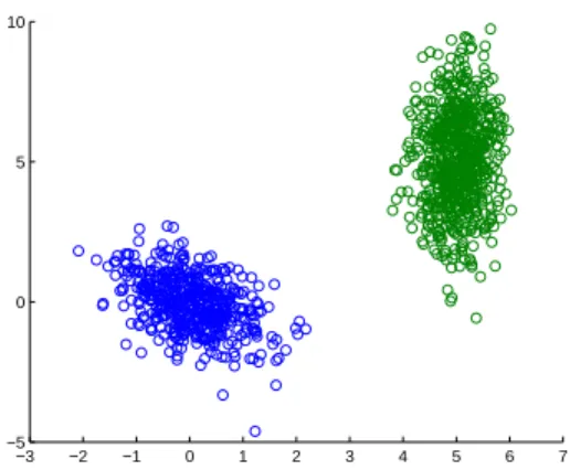
1.1 Example of a dataset withK= 2clusters that are linearly separable. . . 3

1.2 Data drawn from a union of subspaces model. . . 4

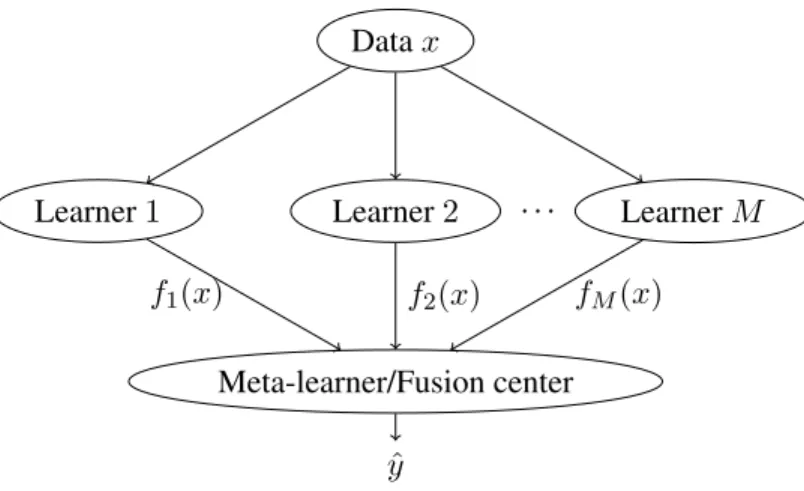
1.3 Unsupervised ensemble learning setup, where the outputs of learners are com-bined in parallel. . . 5

1.4 Example of crowdsourcing for cerebellum segmentation [10]. . . 7

1.5 Named entity recognition example [60]. . . 7

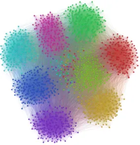
1.6 Example of graph data with8classes. . . 8

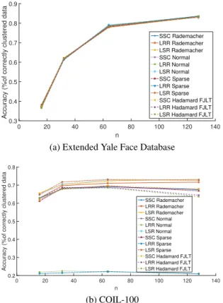
2.1 Simulated tests on real datasets Extended Yale Face Database and COIL-100, evaluating the clustering performance with different JLT matrixR. . . 27

2.2 Simulated tests on real dataset Extended Yale Face Database B, withN = 2,414 data dimensionD= 2,016andK= 38clusters for varyingn. . . 28

2.3 Simulated tests on real dataset COIL-100, withN = 7,200data dimension D= 1,025andK = 100clusters for varyingn. . . 30

2.4 Singular value plots for the Extended Yale Face database and the COIL-100 dataset. . . 31

2.5 Simulated tests on real dataset Extended Yale Face Database B, withN = 2,414 data dimensionD= 2,016andK= 38clusters for varyingdand fixedn= 70. 32 2.6 Simulated tests on ‘Extended Yale Face Database B,’ withN = 2,414data; D= 2,016; andK= 38. . . 33

2.7 Simulated tests on a preprocessed subset of MNIST dataset withN = 5,000 data;D= 500; andK = 10. . . 34

3.1 Unsupervised ensemble classification setup, where the outputs of learners are combined in parallel. . . 36

(12)

ellipses indicate observed variables, i.e. annotator responses. . . 40 3.3 Average estimation errors of confusion matrices (top); and prior probabilities

(bottom), for two synthetic datasets withK = 2andM = 10annotators . . . . 58 3.4 Classification ER for a synthetic dataset with K = 5 classes, priors π =

[0.2404,0.2679,0.0731,0.1950,0.2236]>andM = 10annotators. . . 59 3.5 Classification ER for a synthetic dataset with K = 7 classes, priors π =

[0.2347,0.0230,0.0705,0.1477,0.2659,0.0043,0.2539]>andM = 10 annota-tors. . . 59 3.6 Average estimation errors of confusion matrices (top); and prior probabilities

(bottom) for two synthetic datasets withK= 5andK = 7classes andM = 10

annotators . . . 60 3.7 Classification ER for a synthetic dataset with K = 3 classes, priors π =

[0.2318,0.4713,0.2969]>andN = 106data. . . 62 3.8 Classification ER for a synthetic dataset with K = 5 classes, priors π =

[0.3596,0.1553,0.1229,0.3258,0.0364]>andN = 106_{data. . . .} ₆₂

3.9 Classification ER for a synthetic dataset with K = 5 classes, priors π = [0.3596,0.1553,0.1229,0.3258,0.0364]>andN = 5,000data. . . 63 3.10 Average estimation errors of confusion matrices (top); and prior probabilities

(bottom) for two synthetic datasets withK = 3andK= 5classes andN = 106

data, and a synthetic dataset withK = 5classes andN = 5,000data. . . 63 3.11 Classification ER (top); and time (in seconds) (bottom) for a synthetic dataset

withK = 3classes, priorsπ= [0.3096,0.3416,0.3488]>,M = 30annotators for varying number of dataN and annotator groupsL. . . 64 3.12 Classification ER for a synthetic dataset with K = 3 classes, priors π =

[0.31,0.34,0.35]>,N = 106,M = 10annotators and varying percentage of adversarial annotatorsα. . . 64 4.1 Graphical representation of the proposed model for sequential data. Shaded

ellipses indicate observed variables, i.e. annotator responses. . . 69 4.2 Average F-score for a synthetic dataset withK = 4andM = 10annotators . . 79 4.3 Average estimation errors of confusion matrices and prior probabilities for a

synthetic dataset withK = 4andM = 10annotators . . . 80

(13)

4.5 Average estimation errors of confusion matrices and prior probabilities for a synthetic dataset withK = 2andπ= [0.9003,0.0997]>andM = 10annotators 82

(14)

Chapter 1

Introduction

Data analytics and machine learning already have a ubiquitous presence in our daily lives [29]. Social networking sites, such as Facebook and LinkedIn, analyze user activity and automati-cally adjust the content they offer. Services such as Amazon, Netflix or Spotify automatiautomati-cally recommend new movies and music to their clients based on their past activity and the activity of similar users. Banks and credit companies use machine learning to make credit decisions as well as detect fraudulent activities. E-mail services have developed intelligent algorithms to filter out unwanted emails (spam), but also automatically categorize incoming emails. In order to facilitate all of the aforementioned services, ever increasing amounts of data have to be processed. Aside from their social effect, machine learning and statistical inference have well documented impact in the sciences. As sensors and scientific instruments become increasingly accurate, the data produced by them increases in dimension, requiring increased computational resources for their processing. While the computational demands of modern machine learning and statistical inference tools increase dramatically, the cost of cloud computing is rapidly declining [101]. In addition, the emergent Internet-of-Things (IoT) [153], which consists of numerous connected devices, advocates data analytics methods that minimize the required communication. This prompts us to seek tools that perform efficiently in the highly distributed setups of IoT and cloud computing.

Adding to the challenges posed by the size and volume of the data, machine learning algorithms have been shown to be vulnerable to attacks from adversaries [89]. For example, spammers continuously try to outsmart the spam filtering algorithms deployed by email services. These attacks pose a serious threat, especially in systems where machine learning systems

(15)

perform critical tasks. Therefore, tools that are robust to and can detect adversarial attacks are of paramount importance.

This thesis will leverage contemporary science and engineering tools from disciplines as diverse as optimization, machine learning, signal processing, and big data processing, to put forth analytic and algorithmic foundations for learning efficiently from large volumes of high-dimensional data, possibly in the presence of adversaries.

The major challenge of large-scale learning is to design tools that are fast and efficient yet retain the accuracy of their batch counterparts. Existing approaches [17, 95] have relied on paral-lelization and stochastic optimization to develop efficient machine learning and data analytics schemes. However, parallelizing a large problem typically requires a lot of communication between computing nodes, and stochastic optimization suffers from slow convergence speeds, especially for non-convex problems. Other approaches [18, 151] tackle high-dimensional data by invoking the celebrated Johnson-Lindenstrauss (JL) lemma [67]. These methods reduce the dimensionality of the data by multiplying them with a data-agnostic random projection matrix, and then proceed with the learning task on the dimensionality reduced dataset. This approach however, is not tailored for large volumes of data.

Another approach for large-scale learning is ensemble learning. Ensemble learning is the task of creating a meta-learner, by combining the results of multiple individual learners [33]. Additionally, ensembling can significantly increase the performance of so-called “weak” learners, that is learners performing slightly better than random [44]. Thus, instead of training a highly complex algorithm, one can possibly use an array of simpler algorithms and combine their results in an appropriate manner. At the same time, as different machine learning and statistical inference algorithms operate under different assumptions, there is no “one-size-fits-all” algorithm. By combining the results from multiple algorithms, ensemble learning complements the strengths of each algorithm to produce a result that is better than the results provided from each individual algorithm.

Regarding adversarial machine learning, recent research has mainly focused on deep neural networks [52, 53], with only a few exploring how other machine learning algorithms are affected by adversarial examples [104, 139]. In addition, the effect of adversaries in an ensemble learning setup remains a basically uncharted territory.

The central goal of this thesis is to put forth algorithmic foundations and performance analyses for optimally handling large-scale high-dimensional data as well as dealing with

(16)

−3 −2 −1 0 1 2 3 4 5 6 7 −5

0 5 10

Figure 1.1: Example of a dataset withK = 2clusters that are linearly separable. adversarial agents that seek to undermine the machine learning task. The first line of research will focus on methods to accelerate clustering, and in particular the popular subspace clustering (SC) method, for general and tensor based data. The research in Chap. 2 is geared to address the following question:

• How can we accelerate existing SC schemes while maintaining high clustering accuracy? The second line of research focuses on ensemble learning, and in particular blind (unsu-pervised) ensembles. Blind ensembles are well motivated when there is no knowledge of how different algorithms will perform on a particular dataset, and the meta-learner has no access to ground-truth data. In addition, the blind ensemble learning setup also emerges in fields such as crowdsourcing and distrubuted detection/estimation among others. The key contribution of this thrust will be to show that results from multiple heterogeneous learners can be judiciously combined, even without the presence of ground-truth data at the meta-learner. To this end, our research aims in Chapters 3 and 4 to answer the following question:

• How can we optimally and efficiently combine the answers of multiple algorithms/annotators in the absence of ground-truth data?

• How can we incorporate information about data dependencies in the blind ensemble learning task?

• How does the presence of adversaries affect the ensemble learning task?

(17)

Figure 1.2:Data drawn from a union of subspaces model.

1.1 Large-scale subspace clustering

Clustering (a.k.a. unsupervised classification) is a method of grouping data, without having labels available. Also referred to as graph partitioningorcommunity identification, it finds applications in data mining, signal processing, and machine learning. Arguably, the most popular clustering algorithm isK-means due to its simplicity [57]. However,K-means, as well as its kernel-based variants, provide meaningful clustering results only when data, after mapped to an appropriate feature space, form “tight” groups that can be separated by hyperplanes [57], see e.g. Fig. 1.1. Its scope is further broadened by the so-termed probabilistic and kernelK-means, with an instantiation of the latter being equivalent tospectral clustering– the popular tool for graph-partitioning that can cope even with nonlinearly separable data [32]

Subspace clustering (SC) on the other hand, is a popular method for clustering nonlinearly separable data which are generated by a union of (affine) subspaces in a high-dimensional Euclidean space [145], see e.g. Fig. 1.2. SC has well-documented impact in applications, as diverse as image and video segmentation, and identification of switching linear systems in controls [145]. The more recent SC methods can offer high levels of clustering performance, at the cost, however, of high computational complexity.

(18)

Datax

Learner1 Learner2 . . . LearnerM

Meta-learner/Fusion center

ˆ

y

f1(x) f2(x) fM(x)

Figure 1.3: Unsupervised ensemble learning setup, where the outputs of learners are combined in parallel.

As the main issue with large-scale SC is the huge volume of data, to realize large-scale subspace clustering, this thesis will leverage results from the well-studied field of random projections. Specifically, random projections will be employed to reduce the number of data, while at the same time maintaining high clustering performance. The proposed approach is extended to distributed SC regimes.

1.2 Learning with blind (unsupervised) ensembles

Ensemble learning refers to the task of designing a meta-learner, by combining the results provided by multiple different learners or annotators1; see Fig. 3.1. This meta-learner should generally be able to outperform the individual learners. In particular, ensemble classification refers to fusing the results provided by different classifiers. Each classifier observes data, decides a class (out ofKpossible) each of these data belong to, and provides the meta-learner with those decisions. Such a setup emerges in diverse disciplines including medicine [152], biology [96], team decision making [102] and economics [130], and has recently gained attention with the advent of crowdsourcing [19, 61] as well as services such as Amazon’s Mechanical Turk [75] and Clickworker, to name a few. In the crowdsourcing paradigm, multiple workers/annotators are asked to perform simple tasks and then the annotator answers are fused. Crowdsourcing has been successfully applied for mitosis detection in breast cancer images [80], MRI segmentation [10],

(19)

topic modeling [118], and remote sensing [45] among others. A rrelated problem has been considered in the distributed detection or distributed estimation literature [141]. In this case, sensors are observing a phenomenon, decide which one out ofKpossible hypotheses is true, and transmit those decisions to a fusion center, which has to make a final decision. Additionally, a similar problem, termed theCEO problemor multiterminal source coding, has been considered in the information theory literature, albeit from a coding perspective [12].

When training data are available, a meta-learner can learn how to combine the results from individual classifiers, based on these ground-truth labels [33]. One such approach is boosting [42, 43], where multiple classifiers are combined according to their probability of error on the training set. In the boosting regime, each classifier is also using information from the rest. In many cases however, labeled data are not available to train the combining meta-classifier, or, the individual classifiers cannot be retrained, justifying the need forunsupervised(orblind) ensemble methods. One such paradigm is provided by crowdsourcing, where people are tasked with providing classification labels. Accordingly, in a distributed detection setup, the fusion center might not have access to the sensors, once they have been deployed. The task of blind ensemble classification is then to assess the reliability of each annotator while at the same time fusing their responses. Note that this setup is naturally more resilient to adversarial attacks than traditional machine learning approaches, as adversaries can be detected by the fusion center/meta learner. This thesis will use simple concepts from probability, optimization and detection theory to develop new algorithms that judiciously fuse annotator responses, by taking advantage of the special structure exhibited by annotator moments.

Furthermore, in many cases, there might be dependencies in the considered data. For example, the data might form a sequence. Such a setup arises in many natural language processing tasks such as part-of-speech tagging, where parts of a sentence have to be tagged as nouns, verbs, etc.; named-entity recognition, where the named entities, such as locations or people in a sentence have to be identified; and information extraction, to name a few [100]. In addition, more general dependencies can be captured by a graph, where pairwise relationships between data are encoded in the graph edges. Examples of such data include citation or brain networks to name a few. As will be shown in the subsequent chapters of this thesis, these dependencies can be accounted for in the blind ensemble classification task to enhance classification performance.

(20)

Annotator response 1 Annotator response 2

Annotator response 3 Ground-Truth

Crowdsourcing result

Figure 1.4:Example of crowdsourcing for cerebellum segmentation [10].

Figure 1.5: Named entity recognition example [60].

1.3 Thesis Outline

The remainder of the thesis is organized as follows.

Chapter 2 of the present thesis deals with large-scale subspace clustering. A random projec-tions based approach, termedSketched SC, is developed. The proposed approach “compresses” the data appropriately and can handle both high volumes, as well as high-dimensional data. Fur-thermore, a distributed version of the proposed algorithms is provided. The proposed algorithms are evaluated with a rigorous performance analysis and extended numerical tests on real datasets.

(21)

Figure 1.6:Example of graph data with8classes.

Chapter 3 introduces a novel approach to multiclass blind ensemble classification for inde-pendent and identically distributed (iid) data. The proposed approach is based on the PARAFAC structure of third-order annotator moments and can readily handle multiple imbalanced classes of data. A rigorous performance analysis is provided along with extended numerical simulations on synthetic and real datasets.

Chapter 4 builds upon the algorithms and results of Chapter 3 and introduces blind ensemble classification approaches for non-iid data. Two cases of dependent data are considered: sequential data, for which a moment-based algorithm and an expectation maximization (EM) algorithm are developed; and a generally dependent data case, where the dependencies are captured by a given graph. For the latter, the algorithm of 3 is combined with a novel EM-based algorithm. Numerical tests on synthetic and real data corroborate the effectiveness of the proposed algorithms.

Finally, Chapter 5 presents a concluding discussion of the proposed approaches, along with future research directions.

1.4 Notational Conventions

Unless otherwise noted, lowercase bold letters,x, denote vectors, uppercase bold letters,X, represent matrices, and calligraphic uppercase letters,X, stand for sets. The(i, j)th entry of

(22)

matrixXis denoted by[X]ij; and its rank by rank(X);X>denotes the transpose of matrixX; RD_{stands for the}_{D-dimensional real Euclidean space,}_R

+for the set of positive real numbers.

Prdenotes probability, or the probability mass function;∼denotes ”distributed as,E[·]stands for expectation, andk · kfor the`2-norm. Underlined capital lettersX denote tensors; while

[[A,B,C]]K is used to denote compactly aK-factor PARAFAC tensor [56, 126] with factor

matrices A = [a1, . . . ,aK],B = [b1, . . . ,bK],C = [c1, . . . ,cK], that is [[A,B,C]]K =

PK

k=1ak◦bk◦ck, where ◦denotes the outer product. SymbolI(A) denotes the indicator

(23)

Chapter 2

Large-scale Subspace Clustering

The immense amount of daily generated and communicated data presents unique challenges in their processing. Clustering, the grouping of data without the presence of ground-truth labels, is an important tool for drawing inferences from data. Subspace clustering (SC) is a relatively recent method that is able to successfully classify nonlinearly separable data in a multitude of settings. In spite of their high clustering accuracy, SC methods incur prohibitively high computational complexity when processing large volumes of high-dimensional data. Inspired by random sketching approaches for dimensionality reduction, the present paper introduces a randomized scheme for SC, termed Sketch-SC, tailored for large volumes of high-dimensional data. Sketch-SC accelerates the computationally heavy parts of state-of-the-art SC approaches by compressing the data matrix across both dimensions using random projections, thus enabling fast and accurate large-scale SC. Performance analysis as well as extensive numerical tests on real data corroborate the potential of Sketch-SC and its competitive performance relative to state-of-the-art scalable SC approaches.

For the remainder of this chapterX=UρΣρV>ρ denotes the singular value decomposition

(SVD) of a rankρ,D×N matrixX, whereUρisD×ρ,Σρisρ×ρ, andVρisN ×ρ. For a

positive integerr < ρ, the SVD ofXcan be rewritten as

X=UρΣρV>ρ = [UrU¯r] " Σr ¯ Σr # " V_r> ¯ V_r> # =Xr+ ¯Xr (2.1) 10

(24)

whereΣris anr×rdiagonal matrix with the largestrsingular values ofXin descending order,

and Xr = UrΣrV>r is the best rank-r approximation ofX in the sense thatXr minimizes

kX−XrkF. Accordingly,Σ¯ris a(ρ−r)×(ρ−r)diagonal matrix containing the remaining

singular values ofXandX¯r= ¯UrΣ¯rV¯>r. TheD-dimensional real Euclidean space is denoted

byRD, the set of positive real numbers byR+, the set of positive integers byZ+, the expectation

operator byE[·], and the`2-norm byk · k.

2.1 Preliminaries

2.1.1 SC problem statement

Consider N vectors{xi}iN=1 of sizeD×1drawn from a union ofK affine subspaces, each

denoted byS_k, adhering to the model

xi=C(k)ψ_i(k)+µ(k)+vi, ∀xi ∈ Sk (2.2)

wheredk(possibly withdkD) is the dimensionality ofSk;C(k)is aD×dkmatrix whose

columns form a basis ofS_k; thedk-dimensional vectorψ

(k)

i is the low-dimensional representation

ofxiinSkwith respect to (w.r.t.)C(k); theD×1vectorµ(k)is the “centroid” or intercept of

S_k; and,vi denotes theD×1noise vector capturing unmodeled effects. IfSkis linear, then

µ(k)=0.

Let alsopidenote the cluster assignment vector ofxi, and[pi]kthekth entry ofpithat is

constrained to satisfy[pi]k≥0and

PK

k=1[pi]k = 1. Ifpi ∈ {0,1}K, thenxi lies in only one

subspace (hard clustering), while ifpi∈[0,1]K, thenxi can belong to multiple clusters (soft

clustering). In the latter case,[pi]kcan be thought of as the probability thatxi belongs toSk.

Clearly in the case of hard clustering, (2.2) can be rewritten as

xi = K X k=1 [pi]k C(k)ψ_i(k)+µ(k)+vi. (2.3)

Given theD×N data matrixX:= [x1,x2, . . . ,xN]and the number of subspacesK, the

goal is to find the data-to-subspace assignment vectors{pi}Ni=1, the subspace bases

(25)

their dimensions{d_k}K

k=1, the low-dimensional representations{ψ (k)

i }Ni=1, as well as the

cen-troids{µ(k)}K

k=1[145]. SC can be formulated as follows

min P,{C(k)_}_,_{_ψ(k) i },M K X k=1 N X i=1 [pi]kkxi−C(k)ψ(_ik)−µ(k)k22 subject to (s.to) P>1=1; [pi]k≥0, ∀(i, k) (2.4)

whereP := [p1, . . . ,pN],M := [µ(1),µ(2), . . . ,µ(k)], and1 denotes the all-ones vector of

matching dimensions.

The problem in (2.4) is non-convex as all ofP,{C(k)_}K

k=1,{dk}Kk=1,{ψ (k)

i }, andMare

unknown. It is known that whenK= 1andCis orthonormal, (2.4) boils down to PCA [68]

min C,{ψi},µ N X i=1 kxi−Cψi−µk22 s.to C>C=I (2.5)

whereIdenotes the identity matrix of appropriate dimension. Notice that forK= 1, it holds that

[pi]k = 1. Moreover, ifC(k):=0,∀k, looking for{µ(k)}Kk=1,{pi}Ni=1 withK >1, amounts

toK-means clustering min P,M K X k=1 N X i=1 [pi]kkxi−µ(k)k22 s.to P>1=1. (2.6) 2.1.2 Prior work

Various algorithms have been developed by the machine learning [145] and data-mining com-munity [108] to solve (2.4). Generalizing the ubiquitous K-means [87] theK-subspaces al-gorithm [2] builds on alternating optimization to solve (2.4). ForΠand{d_k}K

k=1 fixed, bases

of the subspaces can be recovered using the SVD on the data associated with each subspace. Indeed, givenX(k) := [xi1, . . . ,xi_Nk], belonging toSk (

PK

k=1Nk = N), a basisC(k) can

be obtained from the firstdk(from the left) singular vectors ofX(k)−[µ(k), . . . ,µ(k)], where

µ(k)= (1/Nk)P_i∈Skxi. On the other hand, when{C

(k)_,_µ(k)_}K

k=1are given, the assignment

(26)

datapoint; that is,∀i∈ {1,2, . . . , N},∀k∈ {1, . . . , K}, we obtain [pi]k=      1, ifk= arg min k0_∈{₁_,...,K_} x˜ (k0) i −C(k 0₎ C(k0)>x˜(_ik0) 2 2 0, otherwise (2.7) wherex˜(_ik):=xi−µ(k)andkx˜(_ik)−C(k)C(k) > ˜

x(_ik)k2is the distance ofxifromSk. Thus, the

K-subspaces algorithm operates as follows: (i) FixPand solve for the remaining unknowns; and (ii) fix{C(k),µ(k)}K

k=1, and solve forP. Since SVD is involved, SC entails high computational

complexity, wheneverdkand/orNkare massive.

A probabilistic (soft) counterpart ofK-subspaces is the mixture of probabilistic PCA [131], which assumes that data are drawn from a mixture of degenerate (zero-variance) Gaussians. Building on the same assumption, the agglomerative lossy compression (ALC) minimizes the required number of bits to “encode” each cluster, up to a certain distortion level [92]. Algebraic schemes, such as generalized (G)PCA approach SC from a linear algebra point of view, but generally their performance is guaranteed only for independent and noise-less subspaces [146]. Additional interesting methods recover subspaces by finding local linear subspace approximations [161]; by thresholding the correlations between data [58]; or by identifying the subspaces one by one [116]. Recently, multilinear methods for SC of tensor data have also been advocated [137]; see also [124, 136, 160] for online clustering approaches to handle streaming data.

Arguably the most successful class of solvers for (2.4) relies onspectral clustering[147] to find the data-to-subspace assignments. Algorithms in this class generate first an N ×N symmetric weighted adjacency matrixWto capture the non-directional similarity between data vectors, and then perform spectral clustering onW. MatrixWimplies a graphGwhose vertices correspond to data and the weight of the edge connecting vertexiand vertexjis given by[W]ij.

Spectral clustering algorithms form the graph Laplacian matrix

L:=diag(W1)−W (2.8)

where diag(W1)is a diagonal matrix holdingW1on its diagonal. The algebraic multiplicity of the0eigenvalue ofLyields the number of connected components inG, while the corresponding eigenvectors are indicator vectors of these connected components [147]. Afterwards, having

(27)

formedL, theKeigenvectors{vk}Kk=1corresponding to the trailing eigenvectors ofLare found,

and K-means is performed on the rows of theN ×K matrixV := [v1, . . . ,vK]to obtain

clustering assignments [147].

Sparse subspace clustering (SSC) [37] exploits the fact that under the union of subspaces model (2.4), only a small percentage of data suffices to provide a low-dimensional affine representation of xi; that is, xi = PNj=1,j=6 iwijxj, ∀i ∈ {1,2, . . . , N}. Specifically, SSC

solves the following sparsity-promoting optimization problem

min Z kZk1+ λ 2kX−XZk 2 F s.to Z>1=1; diag(Z) =0 (2.9)

whereZ := [z1,z2, . . . ,zN]; column zi is sparse and contains the coefficients for the

rep-resentation of xi;λ > 0is the regularization coefficient; and kZk1 := PN_i,j₌₁|[Z]i,j|. The

constraint diag(Z) = 0ensures that the solution of the optimization problem is not a trivial one (Z=I), whileZ>1=1is employed to guarantee that theZfound is invariant to shifting the data by a constant vector [145]. MatrixZis used to create the weighted adjacency matrix

[W]ij := |[Z]ij|+|[Z]ji|. Finally, spectral clustering, is performed onWand cluster

assign-ments are identified. Using those assignassign-ments,Mis found by taking sample means per cluster, and{C(k)_}K

k=1,{ψ (k)

i }Ni=1are obtained by applying SVD onX(k)−[µ(k), . . . ,µ(k)].

The low-rank representation (LRR) approach to SC is similar to SSC, but replaces the`1

-norm in (2.9) with the nuclear one: kZk∗:=Pρ_i₌₁σi(Z), whereρstands for the rank andσi(Z)

for theith singular value ofZ. Specifically, LRR solves the following optimization problem [85]

min

Z kZk∗+

λ

2kX−XZk2,1 (2.10)

wherekXk2,1 :=PN_j₌₁kxjk2, andxj denotes thej-th column ofX.

Another popular algorithm is termed least-squares regression (LSR) [90]. It solves an optimization problem similar to (2.10), but replaces the`1/nuclear norm with the Frobenius one.

Specifically, LSR solves min Z 1 2kZk 2 F + λ 2kX−XZk 2 F (2.11)

which admits the following closed-form solutionZ∗ =λ λX>X+I−1

X>X. Combining SSC with LSR, the elastic net SC (EnSC) approaches employ a convex combination of `1

(28)

-and Frobenius-norm regularizers [38, 103]. The high clustering accuracy achieved by these self-dictionary methods comes at the price of high complexity. Solving (2.9), (2.10) or (2.11) scales cubically with the number of dataN, on top of performing spectral clustering acrossK clusters, which renders these methods computationally prohibitive for large-scale SC. When data are high-dimensional (D ), methods based on (statistical) leverage scores, random projections [18, 59, 110, 149], preconditioning and sampling [112], or our recent sketching and validation (SkeVa) [135] approach can be employed to reduce complexity to an affordable level. Random projection based methods left multiply the data matrixX, with ad×Ddata-agnostic random matrix, thereby reducing the dimensionality of the data vectors fromDtod. This type of dimensionality reduction has been shown to reduce computational costs while not incurring significant clustering performance degradation whend=O(PK

k=1dk)[59]. When the number

of data vectors is large (N ), the scalable SSC/LRR/LSR approach [109] involves drawing randomly n < N data, performing SSC/LRR/LSR on them, and expressing the rest of the data according to the clusters identified by that random draw of samples. While this approach clearly reduces complexity, performance can potentially suffer as the random sample may not be representative of the entire dataset, especially whennN and clusters are unequally populated. Other approaches focus on greedy methods, such as orthogonal matching pursuit (OMP), for solving (2.9) [36, 156]. More recently, an active set method, termed Oracle guided Elastic Net (ORGEN) [157], can be used to reduce the complexity of SSC and EnSC tasks, by solving only for the entries ofZthat correspond to data vectors that are highly correlated.

The present thesis introduces a novel approach based on random projections that creates a compact yet expressive dictionary that can be employed by SSC/LRR/LSR to reduce the number of optimization variables toO(nN)forn < N, thus yielding low computational complexity. In addition, the proposed approach can be combined with random projection methods to reduce data dimensionality, which further scales down computational costs.

2.2 Sketched Subspace Clustering

Consider the following unifying optimization problem

min

(29)

Algorithm 2.1Linear sketched data model for Sketch-SC

Input: D×N data matrixX; Number of columns ofRn; regularization parameterλ; Output: Model matrixA;

1: GenerateN ×nJLT matrixR.

2: FormD×ndictionaryB=XR.

3: Solve (2.12) for the cost in (2.14), (2.15), (2.16) to obtainA.

whereBis an appropriateD×nknown basis matrix (dictionary), h(A)is a regularization function of then×N matrixA,L(·)is an appropriate loss function, andCis a constraint set for

A. Eq. (2.12) will henceforth be referred to asSketch-SC objective. As mentioned in Sec.2.1.2, the ability ofA, obtained from (2.12) to distinguish data for clustering depends on the choice ofh(·), and onB. For SSC, LSR and LRR,B=X,n=N andh(·)isk · k1,1₂k · k2F,k · k∗,

andL(·)is 1₂k · k2 F, 1 2k · k 2 F and 1 2k · k 2 F or 1

2k · k2,1respectively. The constraint set for SSC is

C ={A∈RN×N _:_A>₁₌₁_;_diag₍_A_{) =}₀_}_{, while for LSR and LRR, we have}_C₌_RN×N_.

2.2.1 High volume of data

As the aim of the present thesis is to introduce scalable methods for subspace clustering, the dictionaries considered from now on will haven N, bringing the number of variables to O(nN). In particular, the dictionaries employed will have the form,B:= XR, whereRis a N×nsketching matrix. The role ofRis to “compress”X, while retaining as much information from it as possible. To this end, the celebrated Johnson-Lindenstrauss lemma [67] will be invoked.

Lemma 2.1. [67] Givenε >0, for any subsetV ⊂RN _containing_d_{vectors of size}_N_×₁_,

there exists a mapq :RN →Rn_{such that for}_n_≥_n

0 =O(ε−2logd), it holds for allx,y∈ V

(1−ε)kx−yk2₂≤ kq(x)−q(y)k2₂ ≤(1 +ε)kx−yk2₂. (2.13) In particular, random matrices known as Johnson-Lindenstrauss transforms will be employed since they exhibit useful properties.

Definition 2.1. [151, Def. 2.3], [18] AnN×nrandom matrixRforms a Johnson-Lindenstrauss transform (JLT(ε, δ, d)) with parametersε, δ, dif there exists a function f, such that for any

(30)

ε >0, δ <1, d∈Z₊andd-element subsetV ⊂RN_{, with}_n_{= Ω(}logd

ε2 f(δ)), it holds that

Pr n

(1−ε)kxk2₂≤ kx>Rk₂2 ≤(1 +ε)kxk2₂o≥1−δ for any1×N vectorx>∈ V.

One example of a random JLT matrix is a matrix with independent and identically distributed (i.i.d.) entries drawn from a normalN(0,1)distribution scaled by a factor1/√n[151]. Rescaled random sign matrices, that is matrices with i.i.d. ±1 entries multiplied by 1/√n are also JLTs [1, 18], and matrix products involving these matrices can be computed fast [82]. Another class of JLTs that allows for efficient matrix multiplication includes the so-called Fast (F)JLTs. This class of FJLTs samples randomly and rescales rows of a fixed orthonormal matrix, such as the discrete Fourier transform (DFT) matrix, or, the Hadamard matrix [3,4]; see also [27,113,151] where sparse JLT matrices have been advocated.

The following proposition proved in the appendix justifies the use of JLTs for constructing our dictionaryBin (2.12).

Proposition 2.1. LetXbe aD×N matrix such that rank(X) =ρ, and define theD×nmatrix

B:=XR, whereRis a JLT(ε, δ, D) of sizeN ×n. Ifn=O(ρlog(_ερ/ε2 )f(δ))then w.p. at least

1−δ, it holds that

range(X) =range(B).

This proposition asserts that with a proper choice of the sketching matrixR, the dictionary

B is as expressive asXfor solving (2.12), as it preserves the column space ofXwith high probability. The next proposition provides a similar bound on the reduced dimensionn, when n <rank(X) :=ρ.

Proposition 2.2. LetXbe aD×N matrix such that rank(X) =ρ, and define theD×nmatrix

B:=XR, whereRis a JLT(ε, δ, D) of sizeN×n. Ifn=O(rlog(_εr/ε2 )f(δ)), then w.p. at least

1−2δit holds that kB(V>_rR)†−UrΣrkF ≤(ε √ 1 +ε √ 1−ε+ 1 +ε)k ¯ XrkF.

(31)

Upon constructing aBadhering to Prop. 2.1 or Prop. 2.2, (2.12) can be solved for different choices ofh. Whenh(A) = 1₂kAk2

F, the optimization task (termed henceforthSketch-LSR)

min A 1 2kAk 2 F + λ 2kX−BAk 2 F (2.14) is solved by A∗ = λ λB>B+I−1 B>X, incurring complexity O(n3 +n2D+nDN). Accordingly, ourSketch-SSCcorresponds toh(A) = kAk1 = Pij|[A]ij|and relies on the

objective min A kAk1+ λ 2kX−BAk 2 F (2.15)

that can be solved efficiently to obtainAusing the alternating direction method of multipliers (ADMM) [49], as per [37], or any other efficient LASSO solver. The ADMM solver for (2.15) incurs complexityO(n3+n2D+nDN+n2N I), whereIis the required number of iterations until convergence, and the constraint diag(A) = 0is no longer required as Iis not a trivial solution of (2.15). Proceeding along similar lines, ourSketch-LRRobjective, forh(A) =kAk∗ aims at min A kAk∗+ λ 2kX−BAk 2 F (2.16)

that can be solved using the augmented Lagrange multiplier (ALM) method of [85], which incurs complexityO(n3₊_n2_D₊_nDN_{+ (}_nDN₊_nN2₊_n2_N₎_I₎_{, where}_I_{is the number of iterations}

until convergence. In addition, (2.16) can be solved using the`2,1norm instead of the Frobenius

norm for the fitting termX−BA. The entire process to obtain the data modelAis outlined in Alg. 2.1. Detailed algorithms for solving (2.15) and (2.16) are described in Appendix D. Remark2.1. An optimal data-driven choice ofRwould be interesting only if finding it incurs manageable complexity - a topic which goes beyond the scope of this submission and constitutes a worthy future research direction.

Remark2.2. Upon computingB, (2.14) and (2.15) can be readily parallelized across columns of

X. In the nuclear norm case of (2.16) one can employ the following identity [124, 132] kAk∗ = min Z=PQ> 1 2(kPk 2 F +kQk2F) (2.17)

whereAis somen×N matrix of rankρandPandQaren×ρandN×ρmatrices respectively. This is especially useful when multiple computing nodes are available, or the data is scattered

(32)

across multiple devices. Without (2.17), distributed solvers of (2.16) are challenged because as columns ofAare added the SVD needed to find the nuclear norm has to be recomputed, which is not the case with (2.17).

Remark2.3. Existing general guidelines for choosing the regularization parameterλfor SSC and LRR [37, 85] rely on cross-validation and apply also to the proposed Algs. 2.1 and 2.2 here. 2.2.2 High-dimensional data

The complexity of all the aforementioned algorithms depends on the data dimensionalityD. As such, datasets containing high-dimensional vectors will certainly increase the computational complexity. As mentioned in Sec. 2.1.2, dimensionality reduction techniques can be employed to reduce the computational burden of SC approaches. Using PCA for instance, a d < D-dimensional subspace that describes most of the data variance can be found. This, however, can be prohibitively expensive for large-scale datasets whereN . For such cases, our idea is to combine the method described in the previous section with randomized dimensionality reduction techniques [59]. LetRˇ be ad×DJLT matrix, wheredDis the target dimensionality, and consider thed×N matrixXˇ := ˇRX, which is a reduced dimensionality version of the original dataX. The Sketch-SC objective then becomes

min

A h(A) +λL( ˇX− ˇ

BA) (2.18)

whereBˇ := ˇXR is ad×ndictionary of reduced dimension with R being anN ×n JLT matrix as in (2.12). Upon formingXˇ andBˇ, (2.18) can be solved for different choices ofhas in Sec. 2.2.1. The steps of our algorithm for high-dimensional data are summarized in Alg. 2.2. Remark2.4. While carrying out the productsXR,RXˇ orXRˇ can be computationally expensive in cases, they can be accelerated using modern numerical linear algebra tools, such as the Mailman algorithm [82] or by employing the Welsh-Hadamard transform [77, 112].

2.2.3 Obtaining cluster assignments

After obtaining theN ×N matrixZin (2.9), (2.10) or (2.11), a typical post-processing step for SSC, LSR, and LRR, is to perform spectral clustering, usingW :=|Z|+|Z>|as the adjacency

(33)

Algorithm 2.2Linear sketched data model for Sketch-SC andD

Input: D×N data matrixX; Lower dimensiond; Number of columns ofRn; regularization parameterλ;

Output: Model matrixA;

1: Generated×DJLT matrixRˇ.

2: GenerateN ×nJLT matrixR.

3: Formd×N matrixXˇ = ˇRX.

4: Created×ndictionaryBˇ = ˇXR.

5: Solve (2.18) to obtain sketched data modelA.

matrix. This step however, is not possible for the matrixAobtained from (2.14), (2.15) or (2.16), because it has sizen×N, withn < N.

WhileAcannot be directly used for spectral clustering, ak-nearest neighbor graph [57] can be constructed from the columns ofA. Letaidenote thei-th column ofA, andKithe set of the

kcolumns ofAthat are closest toai, in the Euclidean distance sense. TheN ×N adjacency

matrixWcan then be constructed with entries

[W]ij =    1, ifaj ∈ Kiorai ∈ Kj 0, otherwise. (2.19)

In addition, non-binary edge weights can be assigned as

[W]ij =    wij, ifaj ∈ Kiorai ∈ Kj 0, otherwise. (2.20)

wherewij is some scalar that depends onai andaj. For instance, if heat kernel weights are

used, then wij = exp(−kai−ajk22/σ2), for someσ > 0. The resultant mutual k-nearest

neighbor matrixWcan then be employed for spectral clustering. Note that theN×NmatrixW

emerging from (2.19) or (2.20) will be sparse withO(N)nonzero entries, which can accelerate the eigendecomposition schemes employed for spectral clustering [69, 81]. The overall scheme is tabulated in Alg. 2.3.

Remark2.5. WhenN andnare large, computation of thek nearest neighbors can be com-putationally taxing. Many efficient algorithms are available to accelerate the construction of

(34)

Algorithm 2.3Obtaining clustering assignments fromA

Input: n×N matrixA; Number of nearest neighborsk; Number of clustersK Output: Clustering assignments

1: Findk-nearest neighbors for each column ofA.

2: Create matrixWusing (2.19) or (2.20).

3: Apply spectral clustering onW.

theknearest neighbor graph [5, 107]. In addition, approximate nearest neighbor (ANN) meth-ods [51, 63, 127] can be employed to speed up the post-processing step even further. Finally, this post-processing step can be employed for regular SSC, LSR, and LRR.

2.3 Distributed sketched subspace clustering

In many cases it might be desirable to distribute the computational load of the subspace clustering task to multiple computing nodes. Methods such as SSC and LSR can be easily parallelized, if

Xis available to all computing nodes. However, if the data is scattered across multiple nodes, this approach could incur prohibitive communication and storage costs. Here, we show how the Sketched SC approach can be used to provide communication efficient distributed SC.

Note that upon obtainingB, (2.12) can be readily parallelized across columns ofX. To account for misses, (2.12) is rewritten as

min A∈C h(A) + λ 2kPΩ(X−BA)k 2 F (2.21)

whereΩ ⊆ (1,2, . . . , D)×(1,2, . . . , N)is the set of indices of the observed (non-missing) entries ofX, andPΩis a projection operator such that

[P_Ω(X)]ij :=    [X]ij if(i, j)∈Ω 0 otherwise. (2.22)

Suppose now that data are scattered acrossLcomputing nodes. Each node`has a different subset of the dataX` ⊂Xof sizeN` (PL`=1N` =N). Suppose also without loss of generality

(35)

thatX= [X1,X2, . . . ,XL], in which case B=XR= L X `=1 X`R` = L X `=1 B` (2.23)

whereR` is aN`×nsubset of the rows ofR, andB` :=X`R`is theD×nsubdictionary

corresponding to the`-th computing unit. In order to facilitate a distributed algorithm, each computing node`must find its own subdictionaryB`and communicate it to the remaining nodes,

thus incurring communication complexityO(LDn). For certain classes of JLT, such as those with i.i.d. Gaussian or Rademacher entries, each computing node can generate its ownN`×n

matrixR`, without extra communication overhead. In other cases, a predetermined seed can

be used to generateR`. Upon constructingBas in (2.23), each node`can solve the following

optimization problem min A`∈C` h(A`) + λ 2kPΩ`(X`− L X `0₌₁ X`0R_`0A_`)k2_F, `= 1. . . , L (2.24)

where then×N`matrixA`is the subset of columns ofAcorresponding to the`-th computing

node,C_`is the constraint set forA`, andΩ`⊆(1,2, . . . , D)×(1,2, . . . , N`)is the set of indices

of the observed entries ofX`. The number of variables in (2.24) isO(nN`), which dramatically

reduces the computational burden per node; and, ifhis separable across the columns ofA, then solving (2.24) for`= 1, . . . , Lis equivalent to solving the full problem (2.21). This holds for h = k · k2

F andh = k · k1, whereas in the nuclear norm case one can employ the following

identity [79, 124, 132] kZk∗= min Z=PQ> 1 2(kPk 2 F +kQk2F) (2.25)

whereZis someM×Imatrix of rankρandPandQareM×ρandI×ρmatrices respectively. After finding{A`}L_`₌₁, columns ofA := [A1, . . . ,AL]can be clustered by collectingA

at a fusion center and performing spectral clustering, or, using distributed schemes, such as distributedK-means [8, 39] or distributed spectral clustering [25]. The entire distributed SC process is summarized in Alg.2.4.

(36)

Algorithm 2.4Distributed Sketched Subspace Clustering(SC)

Input: Data matrix per computing node{X`}L`=1; Number of columns of random matrixn;

regularization parameterλ; Output: Clustered data;

1: forcomputing node`do

2: GenerateN`×nJLT matrixR`.

3: CreateD×nsubdictionaryD`=X`R`. 4: TransmitD`to other nodes. Receive{D`0}_`0₆₌_`.

5: FormD=PL

`0₌₁D`0 6: Solve (2.24) and obtainA`. 7: end for

8: Perform spectral clustering on columns ofA= [A1, . . . ,AL].

2.4 Performance Analysis

In this section, performance of the proposed method will be quantified analytically. Albeit not the tightest, the bounds to be derived will provide nice intuition on why the proposed methods work. The following theorem bounds the representation error of Sketch-LSR in the noise less case.

Theorem 2.1. Consider noise-free and normalized data vectors obeying (2.3) withvi ≡0, to

form columns of aD×N data matrixX, with unit`2norm per column, and rank(X) =ρ. Let

alsoRdenote a JLT(ε, δ, D) of sizeN ×n. Letg∗(x) :=Xz∗ =xdenote the representation ofxprovided by LSR, andg(x) :=ˆ XRaˆ the representation given by Sketch-LSR. Ifn =

O(rlog(_εr/ε2 )f(δ)), then the following bound holds w.p. at least1−2δ

kg∗(x)−g(x)ˆ k₂ ≤λ(1 + r 1 +ε 1−ε √ ρ−r σ2_r₊₁) +√ 1 1 +ε

withλas in (2.12), andσr+1denotes the(r+ 1)st singular value ofX.

Theorem 2.1 implies that the largernis, the smaller the upper bound becomes as a smaller singular value ofXis selected. This also suggests that datasets exhibiting lower rank can be compressed more (with smaller n), while retaining representation accuracy. The following corollaries extend the result of Thm. 2.1 to the Sketch-SSC and Sketch-LRR cases.

(37)

of a datum given by Sketch-SSC. The following bound holds w.p. at least1−2δ kg∗(x)−ˆg(x)k2 ≤λ(1 + r 1 +ε 1−ε √ ρ−r σ_r2₊₁) + r n 1−ε

This corollary is a direct consequence of the fact that for anyn×1 vector x, it holds that kxk1≤

√

nkxk2. Accordingly, the following corollary for Sketch-LRR holds because for any

ranknmatrixXwe havekXk∗≤ √

nkXk_F.

Corollary 2.2. Consider the setting of Thm. 2.1, and letg∗(X) :=XZandg(ˆ X) :=XRAˆ

be the representations of all the data given by LRR and Sketch-LRR respectively. The following bound holds w.p. at least1−2δ

kg∗(X)−gˆ(X)kF ≤λ( √ N+ r 1 +ε 1−ε √ ρ−r σ_r2₊₁) + r n 1−ε

For the Sketch-SSC and Sketch-LRR, tighter bounds could possibly be derived by taking into account the special structures of the`1and nuclear norms, instead of invoking norm inequalities.

For a datasetX drawn from a union of subspaces model, batch methods such as SSC, LSR and LRR, should produce a matrix of representations Zthat is block-diagonal, under certain conditions on the separability of subspaces [85, 90]. This, in turn, implies that for data

xi,xj ∈ Sk,x`∈ Sk0 fork6=k0, it holds that

kzi−zjk2 ≤ kzi−z`k2 (2.26)

that is the representations of two points in the same subspace, are closer than the representations of two points that lie in different subspaces. The following proposition suggests that this property is approximately inherited by the Sketch-SC algorithms of Sec. 3.2, with high probability. Proposition 2.3. Considerxi=Xziandxj =Xzj, and their representation provided by SSC,

LRR or LSRziandzj, respectively. Letρ=rank(X)andai,ajbe the representation obtained

(38)

matrixRis a JLT(ε, δ, D). Ifn=O(ρlog(_ερ/ε2 )f(δ)), then w.p. at least1−δit holds that 1 √ 1 +εkzi−zjk2≤ kai−ajk2 ≤ 1 √ 1−εkzi−zjk2.

Proposition 2.3 also justifies the use of thek-nearest neighbor graph as a post-processing step in Sec. 2.2.3.

As will be seen in the ensuing section, the proposed approach has comparable performance to other high-accuracy SC approaches while requiring markedly less time.

2.5 Numerical Tests

The proposed method is validated in this section using real datasets. Sketch-SC methods (termed throught this section asSketch-SSC, Sketch-LSRandSketch-LRR) are compared to SSC, LSR, LRR, the orthogonal matching pursuit method (OMP) for large-scale SC [156], as well as ORGEN [157]. When datasets are large (N ), the proposed methods are only compared to OMP and ORGEN. The figures of merit evaluated are following.

• Accuracy, i.e., percentage of correctly clustered data:

Accuracy:= number of data correctly clustered

N .

• Time (in seconds) required for clustering all data. For Algs. 2.1 and 2.2 this includes the time required to generate the JLT matricesR, the time required for computing the productsB=XR, and in the case of Alg. 2.2Xˇ = ˇRX,Bˇ = ˇXR, as well as the time required for Alg. 2.3.

All experiments were performed on a machine with an Intel Core-i5 4570CPU with16GB of RAM. The software used to conduct all experiments is MATLAB [94]. K-means and ANN were implemented using the VLfeat package [143]. All results represent the averages of10

independent Monte Carlo runs. The regularization scalarλ[cf. (2.9)] of SSC and Sketch-SSC is computed as per [37, Prop. 1], and it is controlled by a parameterα. ORGEN has two parameters that need to be specified, namelyλandα. LRR and Sketch-LRR employ the`2,1norm for the

residualX−XZ. For LRR, LSR, Sketch-LRR, Sketch-LSR, OMP and ORGEN the parameters are tuned to optimize empirically the performance of each method considered.

(39)

The real datasets tested are Hopkins 155 [140], the Extended Yale Face dataset [47], the COIL-100 database [98], and the MNIST handwritten digits dataset [78].

2.5.1 Assessing the effect of different JLTs

Before comparing the proposed scheme with state-of-the-art competing alternatives, the effect of different JLT matrices on the SC task was tested on two datasets: the Extended Yale Face dataset and the COIL-100 database. The differentN×nJLT matrices assessed are: matrices with i.i.d. ±1entries rescaled by1/√n(denoted as Rademacher); matrices with i.i.d. N(0,1)entries rescaled by1/√n(denoted asNormal); Sparse embedding matrices as described in [27, 151] (denoted asSparse); Fast JLTs using the Hadamard matrix as described in [3] (denoted as Hadamard FJLT). Fig. 2.1 depicts the performance of Alg. 2.1 for different choices of JLT for the two aforementioned datasets. All JLT matrices achieve comparable performance for the Yale Face database. However, this is not true for the COIL-100 dataset, where the Rademacher JLT seem to provide the most consistent performance.

For all tests in the rest of this section Algs. 2.1 and 2.2 use random matricesR, andRˇ that are generated having i.i.d.±1entries rescaled by1/√n.

2.5.2 High volume of data

In this section the performance of Sketch-SC (Alg. 2.1) is assessed on all datasets. Hopkins 155 is a popular benchmark dataset for subspace clustering and motion segmentation. It contains 155 video sequences, withN points tracked in each frame of a video sequence. Clusters (K= 2or K = 3) represent different objects moving in the video sequence. The results for the Hopkins 155 dataset are listed in Tab. 2.1 forK = 2and K = 3 clusters, withn = 0.15N for the proposed methods. Here α = 800was used for SSC andα = 100for Sketch-SSC, λ = 1

for LRR andλ= 10for Sketch-LRR,λ= 4.6·10−3 for LSR and Sketch-LSR. The number of nearest neighbors for Alg. 2.3 is set to k = 5. As the size of the dataset is small, large computational gains are not expected by using Alg. 2.1. Nevertheless, the Sketch-SC methods achieve comparable accuracy to their batch counterparts, while in most cases (except one) requiring less time.

The Extended Yale Face database containsN = 2,414face images of K = 38people, each of dimensionD= 2,016. Fig. 2.2 shows the results for this dataset for varyingn, where

(40)

0 20 40 60 80 100 120 140 n 0.3 0.4 0.5 0.6 0.7 0.8 0.9

Accuracy (%of correctly clustered data

SSC Rademacher LRR Rademacher LSR Rademacher SSC Normal LRR Normal LSR Normal SSC Sparse LRR Sparse LSR Sparse SSC Hadamard FJLT LRR Hadamard FJLT LSR Hadamard FJLT

(a) Extended Yale Face Database

0 20 40 60 80 100 120 140 n 0.2 0.3 0.4 0.5 0.6 0.7 0.8

Accuracy (%of correctly clustered data

SSC Rademacher LRR Rademacher LSR Rademacher SSC Normal LRR Normal LSR Normal SSC Sparse LRR Sparse LSR Sparse SSC Hadamard FJLT LRR Hadamard FJLT LSR Hadamard FJLT (b) COIL-100

Figure 2.1: Simulated tests on real datasets Extended Yale Face Database and COIL-100, evaluating the clustering performance with different JLT matrixR.

α = 30for SSC andα = 50for Sketch-SSC,λ= 0.15for LRR and Sketch-LRR,λ = 106

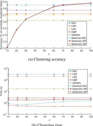
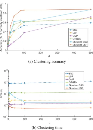
for LSR and Sketch-LSR, the number of non-zeros per column ofZfor OMP is set to5, while λ= 0.7andα= 200for ORGEN. The number of nearest neighbors for Alg. 2.3 is set tok= 5. The proposed algorithms exhibit comparable accuracy to their batch counterparts, in particular SSC, and also achieve higher accuracy than the state-of-the-art large-scale algorithms OMP and ORGEN, asnincreases. Interestingly, withn≈0.03·N the proposed methods achieve the accuracy of batch SSC. In addition, the proposed approach requires markedly less time than the batch methods, and less time than OMP and ORGEN as well.

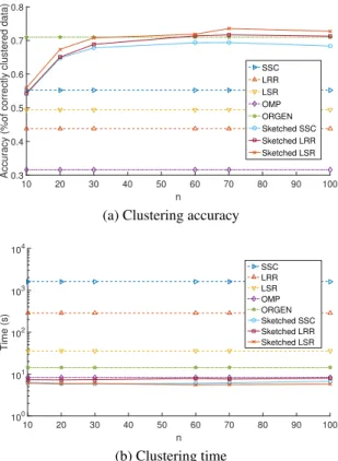
The Columbia object-image dataset (COIL-100) containsN = 7,200images of size32×32

corresponding toK = 100objects. Each cluster corresponds to one object, and contains images of it from72different angles. Fig. 2.3 shows the comparisons on this dataset for varyingn, where α= 25for SSC andα= 500for Sketch-SSC,λ= 0.9for LRR andλ= 10−4for Sketch-LRR,

(41)

10 20 30 40 50 60 70 80 90 100 n 0.2 0.3 0.4 0.5 0.6 0.7 0.8 0.9

Accuracy (% of correctly clustered data)

SSC LRR LSR OMP ORGEN Sketched SSC Sketched LRR Sketched LSR

(a) Clustering accuracy

10 20 30 40 50 60 70 80 90 100 n 10-1 100 101 102 103 Time (s) SSC LRR LSR OMP ORGEN Sketched SSC Sketched LRR Sketched LSR (b) Clustering time

Figure 2.2: Simulated tests on real dataset Extended Yale Face Database B, withN = 2,414

data dimensionD= 2,016andK= 38clusters for varyingn.

λ= 102for LSR and Sketch-LSR, the number of non-zeros per column ofZfor OMP is set to

2, whileλ= 0.95andα= 3for ORGEN. The number of nearest neighbors for Alg. 2.3 is set to k = 5. The proposed approaches exhibit performance comparable to the state-of-the-art asn increases, while requiring significantly less time. Note that, OMP requires almost the same time as the proposed approaches, however its clustering performance is significantly lower.

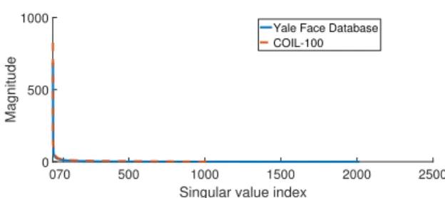
Fig. 2.4 plots the singular values of the Extended Yale Face Database and the COIL-100

dataset. For both, the largest singular values are approximately the first70 ones. Note that for the Extended Yale face database our proposed approaches attain their best performance for approximatelyn = 70yielding a compression ratio of 2414₇₀ ≈34.5, while for the COIL-100 database our proposed approaches reach their peak performance again forn= 70, but this time the compression ratio is 7200₇₀ ≈102.85. This suggests that, indeed, datasets that exhibit low rank can be compressed with a lowern.

(42)

K = 2

Algorithm SSC LRR LSR Sketch-SSC Sketch-LRR Sketch-LSR

Accuracy 0.9839 0.9723 0.982 0.946 0.9435 0.9319

Time (s) 0.6902 0.9478 0.093 0.0795 0.0808 0.0787

K = 3

Algorithm SSC LRR LSR Sketch-SSC Sketch-LRR Sketch-LSR

Accuracy 0.9747 0.9253 0.9654 0.8942 0.9415 0.9242

Time (s) 1.566 1.295 0.1797 0.1755 0.1459 0.1829

Table 2.1: Results forK= 2andK = 3motions for the Hopkins155 dataset

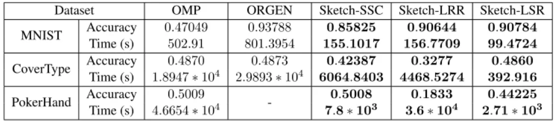
Dataset OMP ORGEN Sketch-SSC Sketch-LRR Sketch-LSR

MNIST Accuracy 0.47049 0.93788 0.85825 0.90644 0.90784 Time (s) 502.91 801.3954 155.1017 156.7709 99.4724 CoverType Accuracy 0.4870 0.4873 0.42387 0.3277 0.4860 Time (s) 1.8947∗104 ₂_.₉₈₉₃_∗₁₀4 _6064.8403 _4468.5274 _392.916 PokerHand Accuracy 0.5009 - 0.5008 0.1833 0.44225 Time (s) 4.6654∗104 _7.8_∗₁₀3 _3.6_∗₁₀4 _2.71_∗₁₀3

Table 2.2: Results for the Preprocessed MNIST dataset (N = 70,000), the CoverType dataset (N = 581,012) and the PokerHand dataset (N = 1,000,000)

ORGEN. The results for the following three datasets are listed in Tab. 2.2. The MNIST dataset contains70,000images of handwritten digits, each of dimension28×28, withK = 10clusters, one per digit. Here the dataset is preprocessed with a scattering convolutional network [21] and PCA to bring each image dimension down toD= 500, as per [156, 157]. Heren= 200, α = 12,000for Sketch-SSC,λ= 1for Sketch-LRR,λ= 10−1 for Sketch-LSR, the number of non-zeros per column ofZfor OMP is set to10, whileλ= 0.95andα= 120for ORGEN. The number of nearest neighbors for Alg. 2.3 is set tok= 3, and the set of nearest neighbors for each datum is found using the ANN implementation of the VLfeat package. In this scenario ORGEN showcases the best clustering performance, however Sketch-LRR and Sketch-LSR exhibit comparable accuracy, while requiring markedly less time.

The CoverType dataset consists ofN = 581,012data belonging toK= 7clusters. Each cluster corresponds to a different forest cover type. Data are vectors of dimensionD= 54that contain cartographic variables, such as soil type, elevation, hillshade etc. Heren= 150,α= 1

for Sketch-SSC,λ= 10−8for Sketch-LRR,λ= 104for Sketch-LSR, the number of non-zeros per column ofZfor OMP is set to15, whileλ= 0.95andα = 500for ORGEN. The number of

(43)

10 20 30 40 50 60 70 80 90 100 n 0.3 0.4 0.5 0.6 0.7 0.8

Accuracy (%of correctly clustered data)

SSC LRR LSR OMP ORGEN Sketched SSC Sketched LRR Sketched LSR

(a) Clustering accuracy

10 20 30 40 50 60 70 80 90 100 n 100 101 102 103 104 Time (s) SSC LRR LSR OMP ORGEN Sketched SSC Sketched LRR Sketched LSR (b) Clustering time

Figure 2.3: Simulated tests on real dataset COIL-100, withN = 7,200data dimensionD = 1,025andK = 100clusters for varyingn.

nearest neighbors for Alg. 2.3 is set tok= 10, and the set of nearest neighbors for each datum is found using the ANN implementation of the VLfeat package.

The PokerHand database containsN = 106data, belonging toK = 10classes. Each datum is a5-card hand drawn from a deck of52cards, with each card being described by its suit (spades, hearts, diamonds, and clubs) and rank (Ace, 2, 3, . . . , Queen, King). Each class represents a valid Poker hand. Heren = 30, α = 10for Sketch-SSC, λ = 1for Sketch-LRR,λ = 102

for Sketch-LSR, the number of non-zeros per column ofZfor OMP is set to10. The number of nearest neighbors for Alg. 2.3 is set tok = 20, and the set of nearest neighbors for each datum is found using the ANN implementation of the VLfeat package. Results are not reported for ORGEN as the algorithm did not converge within24hours. For both the CoverType and PokerHand datasets, most algorithms exhibit comparable accuracy, while Alg. 2.1 requires again less time than OMP or ORGEN.

(44)

070 500 1000 1500 2000 2500 Singular value index

0 500 1000

Magnitude

Yale Face Database COIL-100

Figure 2.4: Singular value plots for the Extended Yale Face database and the COIL-100 dataset. 2.5.3 High-dimensional data

In this section, the performance of Sketch-SC approaches combined with randomized dimension-ality reduction (Alg. 2.2) is assessed, for the Extended Yale Face database.

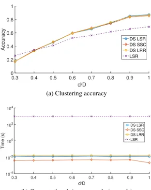
Fig. 2.5 depicts the simulation results on the Extended Yale Face database, when performing dimensionality reduction, for varyingd. Here Alg. 2.2, with fixedn = 70is compared to its batch counterparts, OMP and ORGEN. LRR and Sketch-LRR are not included in this simulation as the algorithm failed for small values ofd. All parameters are the same as the corresponding experiment in Sec. 2.5.2. In this experiment, Sketch-LSR and Sketch-SSC outperform their competing alternatives in terms of clustering accuracy, while maintaining a low computational overhead. OMP also exhibits low computational time, at the expense of clustering accuracy. 2.5.4 Distributed SC

Next we evaluate the performance of the proposed Distributed sketched SC scheme, using real datasets. Let d denote the number of observed entries per column of X. Distributed sketched SC methods (denoted byDS-LSR, DS-SSCandDS-LRR) are compared to batch LSR [cf. (2.21)] across variable percentages of available datad/D. The metrics evaluated are the clustering accuracy, expressed as the percentage of correctly clustered data given by the rate

(number of data correctly clustered)/N, and the computational time per node in seconds, that is the average time required by a single node to solve (2.24). TheD×N datasetXis distributed acrossLdifferent computational nodes, each required to process approximatelyN` =bN/Lc

data. TheN ×nrandom matricesRin all experiments have i.i.d. normal entries rescaled by a factor1/√n. As matrixAresulting from Alg. 2.4 is notN×N, ak-nearest neighbor (k-NN) graph, with adjacency matrixW, is created using the columns ofA. The edge weights of this graph are given by[W]ij = exp(−kai−ajk22/2σ2), whereaiis one of theknearest neighbors