Housing price development in Shanghai
Master’s Thesis
Department of Built Environment School of Engineering
Aalto University
Espoo, 27 May 2019
Lili Tian
Master of Science in Technology Lili Tian Supervisor: Professor Heidi Falkenbach Advisor: Professor Heidi Falkenbach
Aalto University, P.O. BOX 11000, 00076 AALTO www.aalto.fi Abstract of master's thesis
Author Lili Tian
Title of thesis Housing price development in Shanghai
Master programme Real Estate Economics Code ENG24
Thesis supervisor Professor Heidi Falkenbach
Thesis advisor(s) Professor Heidi Falkenbach
Date 27.05.2019 Number of pages 38 Language English
Abstract
Rapid increase in housing prices and growing mortgage lending aroused great concern of whether there is bubble in Chinese housing market. In fact, the price-to-rent ratio and price-to-income ratio soar in most Chinese cities, especially in coastal- and some inland- areas, making housing affordability a prominent issue. The thesis tends to examine housing price movement in Shanghai over years 2002 to 2017 in order to reveal whether there was a bubble in Shanghai housing market and the possible implications. Measures like price-to-rent ratio, price-to-income ratio and cointegration test are employed to reflect the interaction between house price and market determinants like disposable income, GDP and land price etc. The house price movement shall be taken with caution in order to develop a dynamic housing market.
Keywords Shanghai housing price, housing bubble, cointegration test, price-to-income ratio
Table of Contents
1. Introduction ... 1
1.1. Background... 1
1.2. Research Questions and Goals ... 3
1.3. Research Scope and Delimitation ... 3
1.4. Structure ... 4
2. Bubbles in housing markets ... 5
2.1. Determinants of housing price ... 5
2.2. Housing bubble ... 7
2.3. Measuring house price bubbles ... 11
3. Features of the Chinese housing market ...17
3.1. Housing and land use rights reform ... 17
3.2. Housing policies ... 20
4. Data and Methodology ...22
4.1. Data ... 22 4.2. Methodology ... 22 5. Preliminary Analysis ...24 6. Discussion ...31 6.1. National Economy ... 31 6.2. Banking System ... 31 7. Conclusion ...33 7.1. Evaluation of research ... 33 7.2. Future research ... 33 References ...35
1
1. Introduction
1.1. Background
During the past decades, China’s residential property market has developed greatly. Housing
prices grew at an ever-increasing rate in coastal cities and some inland areas. Figure 1 displays the price index from the China Real Estate Index System (CREIS) of newly-constructed dwellings across eight major Chinese cities. The Beijing housing price index points were 1,224 in January 2005, and it rose by 227 percent to 4,000 points in December 2015. The indexes of Shenzhen and Shanghai were higher than that of most cities, with a growth rate of 199 and 81 percent, respectively, during the 2005-2015 periods. The indexes of the other cities, such as Nanjing, Hangzhou and Wuhan were lower but still with a growing trend. The figure indicated that the development of the housing market was not a city-specific event but seemed like a country-wide phenomenon. Besides, the price-to-income ratio (P-I ratio), which represents the affordability of housing, surged considerably in most cities; as a result, the average housing price climbed to an unbelievable high that most individuals believe they cannot afford. All these changes aroused great concern of the housing price bubble in China and the sustainable development of the Chinese residential property market.
Figure 1 House Price Index from CREIS of eight Chinese cities from 2005 to 2016 Source: China Real Estate Index System
Along with the soaring housing market, the Chinese economy experienced rapid growth during 2001-2015. The average annual GDP growth rate maintained over 7 percent, and between 2004 and 2009, the growth rate was even more than 10 percent (China Statistical Yearbook, 2001-2016). The output of the construction industry in 2015 constituted 6.9 percent of the Chinese GDP (China Statistical Yearbook, 2016). The prosperous economy interacts with the development of the real estate sector. Real estate investment was one of the
0 1000 2000 3000 4000 5000 6000 H ous e P rice I nd ex Shanghai Beijing Guangzhou Shenzhen Wuhan Nanjing Hangzhou Chengdu
2
major sources for economic growth, and the booming economy contributed to the real estate sector. During the last decade, real estate investment experienced remarkable growth; by the end of 2015, investment reached RMB 9597.8 billion nationally, accounting for 17.4 percent of the total fixed investment, while residential property investment was about RMB 6459.5 billion, constituting 67.3 percent of total real estate investment (China Statistical Yearbook, 2016). The property investment significantly improved the economy by increasing the employment rate and consumptions.
The vast growth in housing supply and housing sale (Figure 2) demonstrated the prosperity of the housing market again. The housing supply surged at an incredible rate during 2005-2011. In following years, with the restricted speculation on land, the land market became rational, and the housing supply decreased. The number for housing sold increased year by year, mainly resulting from fast urbanization and speculation of the housing market.
Figure 2. Supply of new residential housing in China, 2005-2015
Source: China Statistical Yearbook, 2016
In Shanghai, residential property investment totals 181.33 billion, making up 2.81 percent of
the nation’s investment (Shanghai Statistical Yearbook, 2016). The substantial amount of
capital poured into the property industry suggested the boom of the Chinese housing market, and was supposed to have inflated the housing value. In addition, the land sales, which are an important source of revenue for local government, is decreasing in mega-cities, and the land value is becoming more overpriced, which lays the foundation for higher housing prices. In Shanghai, for example, land sales accounted for as much as 35 percent of government general revenue. The land value reached 30 percent to 40 percent of the housing price, which is
0 20000 40000 60000 80000 100000 120000 140000 160000 2005 2006 2007 2008 2009 2010 2011 2012 2013 2014 2015 Housing started area(ten thousand sq m) Housing sold area(ten thousand sq m)
3
considerably large. On the other hand, from 2008 to early 2010, the ratio of land price to house jumped to 60% (Wu et al., 2010), which consequently delivered the high house price. Except the exuberance of the economy, the urbanization in China is increasing. People moved from rural areas to urban cities, and a large amount of individuals migrated from inland areas to developed coastal cities. The population of Beijing, Shanghai and Shenzhen each surpassed 20 million and became the mega-cites. The demand of housing in large- and medium-sized cities was considerably high and is continuously growing because of urbanization.
With demand growing and the expectation of house price increases in mega-cities, the price of residential properties is posed to increase. However, with the slow growth of household income, the housing affordability will become severe and be a prominent issue in current China, as the housing price not only affects households’ well-being, but also plays a vital role in the soundness of the economy.
As demonstrated in the last global financial crisis, housing price volatility contributes to risks for the banking system. Financial crisis resulting from excessive issuance of mortgage-based securities dramatically lowers the property prices, which crashed the banking system in the US and the UK. Though China avoided a crisis in housing market and banking industry, it reveals that the market is vulnerable when risks occur. As China’s bank lending is booming
and mortgage loans soar (loans to property developers and mortgages together occupied 16 percent of total funds by 2013) (Shanghai Statistical Yearbook, 2014), the concern of excessive exposure of bank in the real estate industry argues the possibility of a housing bubble and the risks of financial crisis.
1.2. Research Questions and Goals
As China’s housing market developed rapidly and housing prices in mega-cities reached
highs, the study of real house price movement is a prominent issue. Here, I will study the housing price development in Shanghai between years 2002-2017, and answer the following two questions:
a) Was there a bubble in the Shanghai housing market? b) Which factors contribute to the increasing housing market?
1.3. Research Scope and Delimitation
This thesis studies well-developed mega-cities like Shanghai as they are more representative of the Chinese housing market. Here, only the housing price movement in urban areas in Shanghai are included. Only the residential property market is analyzed. The primary housing market is mainly discussed, but the secondary housing market is not considered. Only
non-4
subsidized housing units are analyzed; the subsidized and price-restricted dwellings are not taken into consideration. The mass property market is examined, and the high-end/luxury properties are excluded. The study only reflects the housing price volatility during years of 2002-2017.
1.4. Structure
This thesis starts by describing the determinants of house price and factors contributing to house bubbles in section 2. Section 3 narrates the housing market development in China and the policies issued by government to lead to sustainable development of the housing market. Section 4 and 5 study the house price movement in Shanghai by using P-R ratio, P-I ratio and cointegration test. Section 6 discusses the implications of house price change on the national economy and banking system. Section 7 shows further research.
5
2. Bubbles in housing markets
2.1. Determinants of housing price
The determinants of house price development are classified into two groups: one that reflects the changes in economic fundamentals, like the growth in real construction costs and in income, and the change in real after-tax interest rate; and the other that states adjustment dynamics, like lagged real appreciation, and the difference between actual and equilibrium housing price levels (Abraham & Hendershott, 1994; Case & Shiller, 2003; Capozza, Hendershott, & Mack, 2004; Goodman & Thibodeau, 2008).
For the first group, it was demonstrated by Case and Shiller (2003) that fundamentals, such as personal income, population, employment rate, unemployment rate, housing starts and
mortgage interest rate, have impacts on long-run house prices. It was revealed by employing reduced form regressions that the growth in income significantly explained housing price increase in most states in the US. However, when it came to the states located in coastal areas, the income pattern could only explain half of the housing price change, with the rest attributed to other economic fundamentals, like housing starts having a negative effect on house price. The paper concluded that there might have been housing bubbles in coastal states between 2000-2002.
Further, the determinants in first and second groups are studied by Abraham and Hendershott, and Goodman and Thibodeau. Abraham and Hendershott (1994), using reduced form
regressions, found that the real income growth, changes in user cost, the supply constraints of housing by either limited land availability or costly building requirements, and lagged
appreciation rate led to the booming house prices in two coasts in the US during the middle and late 1980s. Additionally, they revealed that the intense decrease of housing prices
occurred three to six years after the boom ended, and the adjustment of falling housing prices sustained a very long period of up to a dozen years. Goodman and Thibodeau (2008)
investigated the impact of economic fundamentals, such as change in income, user cost, population, household size, construction cost and agricultural land price speculation on housing price between 2000 and 2005. They found that spatial variance in supply elasticity accounted for spatial variance in housing price appreciation rates; on the East coast and in California, inelastic supplies, owing to rising land prices and housing construction costs, contributed to the large housing price increase of owner-occupied housing. Finally, Goodman and Thibodeau set a housing bubble threshold of 30 percent over difference between observed and expected housing price (but without justification of this parameter) and found that 25 out of 84 metropolitan areas were identified with severe speculative activities.
6
Researchers studied the determinants of Chinese housing price as well. Hui and Yue (2006) applied a variety of econometric methods, such as the Granger causality test, impulse response analysis, and the reduced form equation, to test the effect of changes of market fundamentals (like GDP, disposable income, stock of vacant new dwellings, and Shanghai stock price index) on housing prices movement in Beijing, Shanghai, and Hong Kong. It was said that the growth of disposable income has a positive effect on house price, and the vacant dwellings and stock price index have a negative effect on house price. The paper concluded that a housing price bubble accounted for 22 percent of the price in Shanghai in 2003. Aside from factors like the changes of economic fundamentals, like the GDP, disposable income, construction cost, and supply elasticity, Wu et al. (2012) analyzed the impact of land value appreciation on housing price volatility in China. They concluded that in Beijing, along with the increasing house price, the land price rose dramatically at an average growth rate of 28 percent between 2003 and 2010. They also reported that land purchase price by central state-owned real estate developers was 27 percent higher than the normal developers, and the expectations of housing price appreciation for real estate developers led to the overpricing of land value. By using two housing affordability metrics—price-to-rent and price-to-income ratios—Wu and his colleagues found that the coastal cities in China experienced housing booms, and a small decline in expected appreciation was likely to cause large drops in housing value.
The factors determining China’s property prices were also examined by Ahuja et al. (2010).
They related demand- and supply-side factors like lending interest rate, population density, real GDP per capita, and land prices to housing price misalignment in China from 2000 to 2009. By employing panel regression and the asset pricing method, they revealed that before 2006, the overall property prices were generally in line with the equilibrium values. However, coastal cities and some inland areas, including Beijing and Shanghai, seemed to have
experienced large home price appreciations. Further, they concluded that real property price was not significantly inflated in the first half of 2010, and housing prices were quickly
corrected in an average of half of a quarter, partly due to housing policy executed to settle the housing market.
In conclusion, factors affecting housing price are changes of economic fundamentals, like disposable income, the increase of construction cost, housing stock, land value and so on, and adjustment dynamics, like lagged real appreciation. With change of GDP and income,
construction cost alleviation, limited housing supply, land value appreciation, lower mortgage interest rate, and more, house price fluctuates.
7
2.2. Housing bubble
In asset market, the term “bubble” is explained by Ernan Haruvy et al. (2007) that people’s
long-run price expectations form and sustain the price bubble. People build their predications on past data and previous experience and would optimize investments according to market
changes. With the changing markets and individuals’ expectations, the earlier small bubbles
and former price peak times impact the price forecasting in the next periods and in other markets. Once people perceive a price increase is negligible, they tend to decrease purchases and raise sales; consequently, the market peaks occur earlier and cannot sustain the downturn that follows.
In the housing market, there is no standardized definition of the term “bubble,” but it is widely used and often points to circumstances where the excessive expectations of people of future home price appreciation lead to temporary home price increases (Stiglitz, 1990; Case & Shiller, 2003).
During a housing price boom, people believe a property that is excessively expensive for them is now worth investing in as they expect the future price increases would compensate them. Some homebuyers would think that if they do not buy a house now, they would not get on the
“property ladder” when the housing price soars to unbearable highs. In addition, people who
possess extra capital would like to invest in property assets as they believe property value is less likely to drop; consequently, this contributes to speculative investment and overestimated property value. Therefore, the expectations of fast and stable future price gains are critical factors motivating housing booms and bubbles.
When housing prices cannot rapidly increase or cannot meet the inflated expectations, people are likely to lose faith in the price development and would divest. Subsequently, the support for higher price opportunities breaks down and home prices fall to an extent that causes the bubble to burst (Case & Shiller, 2003).
Despite that excessive public expectations of future home price run-ups cause the housing bubble, many other factors could drive housing prices to a hike and finally the bubble bursts. The stimulators are argued in two aspects although they vary from country to country or region to region. From the demand point-of-view, a rise in consumer needs and changes in fundamentals of housing demand could effectively push booming prices to bubbles; from the supply side, the inelastic housing supply, an increase in the supply of housing finance, monetary and regulatory policy, etc., could have a critical impact on pricing the house (Case & Shiller, 2003; Glaeser, Gyourko, & Saiz, 2008; Levitin & Wachter, 2011; Howden & Li, 2015).
8
From the demand perspective, changes of economic fundamentals could lead to booming demand and thus higher price. Case and Shiller (2003) illustrated that eight areas in the US, such as New England, New York, New Jersey, California, and Hawaii, were more likely to experience housing price volatility when compared with other states between 2000-2002, and that prices developed in line with the increase of income and population. Glaeser, Gyourko, and Saiz (2008) found that areas with growth in population and income, but with inelastic housing supply, were more prone to housing price appreciation. Howden and Li (2015)
believed that the inelastic demand of housing caused the real estate boom in China. In the past two decades, China experienced rapid urbanization, and the demand for houses greatly
increased. Meanwhile, the Chinese perceive that they need to buy a house before marriage. Besides, in order to hedge against increasing high inflation, people would like to invest in properties.
From the supply perspective, the causes of a bubble could be the inelastic housing supply and oversupply of housing-finance. In China, almost all land is owned by the government, and the government generates revenue by leasing land. In early 2004, the Chinese government
launched several policies to ease the prosperous housing market fueled by public housing reform. It required the local authorities to tighten the land supply for housing development. With land-use monopoly, the land price was overvalued, and new housing supply was limited, leading to the overpriced houses between 2004-2007 (Deng et al., 2009). Oizumi (1994) found that inelastic housing supply resulted from land use regulations exacerbated housing market in Japan in the 1980s. In terms of the housing finance, taking the US housing bubble as an example, Levitin and Wachter (2011) asserted that the housing-finance vehicles shifted from traditional fixed-rate mortgages (FRMs) to nontraditional adjustable-rate mortgages (ARMs), and between 2001-2007, housing-finance demand derived from irrational consumers who sought for more financing to fund elevating house prices increased. However, the
increase of housing-finance supply was much larger than that of housing-finance demand. The excessive supply of housing-finance was caused by the loose lending standards (explained later), so that sub-prime borrowers were qualified for loans. Before the 2008 US financial crisis, the typical American house price increased greatly. People could either refinance their homes at lower interest rate or apply for second mortgages secured by price run-ups. With the cool-down of the housing market and the increase of mortgage interest rates, borrowers with ARM could not afford the payments and/or refinance to avoid higher payments associated with rising interest rates. Mortgage loans began to default. Lenders began foreclosure proceedings on properties, which finally led to the collapse of the financial market. The housing finance system in China is severely regulated and relatively simple. The maximum loan-to-value (LTV) ratio in Shanghai is 65 percent. The mortgage term could be as long as
9
30 years. The Chinese banks issue mortgages according to the applicants’ credit-worthiness
and usually adjust risk levels of borrowers. The default rate in China is quite low. For instance, the delinquency rate was only 1.5 percent in 2004 (Deng & Fei, 2008). Thus, the
supply of housing finance was not the main reason for elevating China’s housing prices.
The government lending and affordable housing policy could encourage financial institutions to lend to low- and middle-income households, which consequently elevates the housing price. In the US, the affordable-housing goals of government-sponsored entities (GSEs) were known to have transmitted laxer lending standards to the prime market and fueled provision of credits. In order to improve the homeownership and the access to credit among the lower-income households, the GSEs raised the proportion of loans subjected to underserved borrowers, and relaxed the underwriting terms to enable purchase of riskier loans, such as nontraditional and subprime mortgages (Wallison, 2009). The situation in China was different. The economic and comfortable housing program (ECH, explained in section 3), aimed to stimulate housing consumption, was not well implemented. Usually, the price of ECH is lower than the market price and only middle- and lower-income households could purchase. In reality, the price of ECH was higher than expected and only wealthy households could achieve them (Deng et al.,2009) The ECH program failed to fuel the housing market in China.
The monetary policy is considered to play a role in elevating housing bubble. In China, the M2 increased by over 800 percent since 2000, and the ratio of M2 to M1 money supplies has considerably grown since 2010 (Howden & Li, 2015). Meanwhile, in 2008, the Chinese government launched 4000 billion yuan into the market in order to stimulate the economy. The lax monetary policy and limited investment opportunities make real estate an attractive alternative when compared to bank deposit rates and restricted overseas investments
(Cumming et al., 2013). Low interest rates ensure cheap mortgage costs, which drive excessive demand for loans. As most homebuyers would employ mortgage loans to fulfill their purchase, the lower costs of mortgages would stimulate greater leverage and increase
customers’ purchasing power. Inevitably, the housing prices increase, and bubbles are likely
to form (Taylor, 2013). In China, the interest rate declined from approximately 15 percent in the mid-1990s to around 5 percent in the 2000s (People’s Bank of China, 1998-2017). In Japan, the interest rate decreased from 8% in 1980 to less than 4% during housing bubble period and run up in the 1990s (Shimizu and Watanabe, 2010). The low interest rate
encouraged people to invest in assets like houses by lending more instead of saving. However, when short-term interest rates move to normal levels, housing demand quickly declines, leading to the falling construction and housing prices.
10
Additionally, the global supply of credit could contribute to the housing boom. Savings from foreign countries flow to thriving real estate markets to seek investment opportunities and to simultaneously decrease interest rates, therefore stimulating the housing bubble (Bernanke et al., 2011). As explained by Cumming and his colleagues (2013), the PBoC kept the fixed exchange rate at an underestimated level. Foreign capital flowed to China into safer assets, such as real estate. Meanwhile, the domestic investors were willing to get an additional yield from MBS and therefore guaranteed an affluent supply of mortgage credits.
As mentioned above, the relaxation of underwriting standards of securitization inflated the housing bubble. Favilukis et al. (2011) showed how the housing finance market was when the underwriting terms deteriorated by the end of 2006 in the US. Americans typically purchased houses with a 100% finance option by using a piggyback second mortgage or home equity loan. Borrowers could obtain loans for 125% of the home value if they could use the top 25% to pay for existing debt. In China, most buyers receive loans from four state-owned banks, and the less creditworthy could approach mortgage loans from private lending companies. Such behaviors significantly exaggerated the risks in the housing finance market, and when housing prices became volatile and began to fall, mortgages were more likely to default, consequently having a devastating impact on the housing and financial market.
In sum, factors contributed to the housing bubble were diversified. The excessive expectations of future house price appreciation boomed the residential market. A rise in demand and
inelasticity of housing supply, an increase in the supply of housing finance, relaxed monetary and regulatory policy, the use of easy-to-qualify underwriting and appraisal systems, etc., interactively pushed the house price to a peak.
The impact of bubble-induced recession
Repercussion of a housing bubble are devastating. The burst of a housing bubble and
excessive mortgage lending could lead to financial bubbles. Taking the US housing market as an example, home prices boomed in 2005 and ARM rates began to reset at higher interest rates. The affordability of debt declined and loans began to default. Lenders claimed foreclosure proceedings and people lost home ownership. Home prices depreciated by the increasing inventory of houses offered for sale. With more-than-expected foreclosure rates, the US subprime mortgage industry collapsed. Subprime lenders declared bankruptcy,
announcing great losses. MBS, which is widely invested by financial firms, lost most of their value. Further, concerns about the soundness of US credit and financial market led to
tightening credit and triggered global economic recession. The unemployment rate increased. The US lost over 2.1 million manufacturing jobs and more than 1.8 million construction jobs between December 2007 and November 2009 (US Bureau of Labour Statistics, 2007-2009).
11
A housing bubble generates widespread attention and could cause a severe downturn of the financial market and global economy; therefore, it is crucial to reform space and asset markets so as to prevent a crisis from recurring and to develop a sustainable housing and financial market.
2.3. Measuring house price bubbles
Conventional methods for evaluating pricing in the housing market are price-to-rent ratio, price-to-income ratio, and user cost.
Ratio Method
“P-R ratio measures the relative cost of owning versus renting.” Essentially, when house
prices increase greatly, relative to renting, many more people tend to rent rather than buy. Gradually and consequently, the demand for owner-occupied housing reduces and house prices realign with renting. One benefit of this ratio is that if house prices increase for a long period, it suggests that the high housing price was fueled by excessive expectations of future house price growth rather than the fundamental rental value, therefore generating a bubble.
However, there is one drawback concerning this ratio, in that “it assumes constant risk premia
and rental increase expectations” (Bourassa et al., 2016).
“P-I ratio provides a measure of local housing costs relative to the local ability to pay.” When
household income increases, the affordability of house increases, thus inducing the growing demand of housing, which leads to the upsurge of housing prices. When prices reach as high as the growing household income, the housing affordability becomes severe, implying an overpricing of the house (or probably the emergence of a bubble). Subsequently, the down payments and monthly mortgage payments become so high that the demand for housing gradually reduces; consequently, housing prices move to a normal level. One concern of P-I ratio is that the relationship between prices and income is assumed to be constant and the effect of population change on prices is not considered (Bourassa et al., 2016).
Though there is imperfection in metrics like P-R ratio and P-I ratio, they are reliable
indicators to a degree for explaining the development of housing prices. An increase in price growth rate, a growing cost of obtaining housing, etc. would provide reasons to suspect overvaluation or undervaluation in housing markets. However, further study is needed in order to improve the accuracy of measurement of a speculative bubble.
User cost, which is also known as imputed rents (compared to actual rents available in the market), is another method to measure price change. “Imputed rents are defined as the
12
the real price level” (Bourassa et al., 2016). In a well-functioning housing market, the house rental market and capital market are relatively stable, and the cost of owning a house (imputed rent) is more or less equal to that of renting a similar house during the same duration. If the cost of renting is considerably higher than ownership, individuals would rather buy a
property. On the other hand, if the ownership cost is much higher than renting, people would gradually go to the rental housing market. The gap between cost of renting and ownership leads to arbitrage in the housing market. One point to emphasize here is that even in an efficient market, there are additional costs, such as moving costs, transaction commission, etc., making the imputed rent and market rent disequilibria. Thus, the small and/or short-time deviation between these two are not taken into account, but there is a sizable and persistent gap.
User costs of owning can computed by a formula pioneered by Poterba (1984). The annual cost of ownership is a sum of six components:
ut = (1–τt) (rtm+ wt) + δt – Etgt+1 + pt (1) Rt = Pt∗ut (2)
where ut,,τt, rtm, wt, δt, Etgt+1 and pt respectively denote the annual total user cost in the form of cost per monetary unit of house price, the income tax rate, mortgage interest rate, the property tax rate, maintenance cost as a fraction of home value, expected annual capital gains, and an additional risk premium. Rt, Pt∗and respectively denote market rent, benchmark house price. Himmelberg, Mayer, and Sinai (2005) compared user cost to local incomes and actual rent and found that the housing market did not seem as overpriced in 2004 as it looked in most US cities.
Other approaches to measuring housing prices or bubbles are based on regression analysis of various forms. The three most popular types are models based on housing supply and demand fundamentals, asset pricing, and cointegration and unit root tests (Case & Shiller, 2003; Bourassa et al., 2016).
Housing Price and Fundamentals
The first model, the long-term relationship between equilibrium house price and economic fundamentals, assumes that the change of economic fundamentals has an impact on housing supply and demand, thus affecting the housing price. Then, if the actual price level deviates from the equilibrium level too much and sustains for a period, it is argued that the housing market is too volatile, and there are housing bubbles.
The model for comprehending the fundamentals affecting housing supply and demand is as follows:
13 Pt∗ = a0 + a1D t ∗ + a2y t∗ + a3rt∗ + a4L∗t + a5et∗ + a6ct∗+ …+ anVt∗ (1) Pt = Pt∗+ θt (2) where t represents time period, Pt∗, P
t expresses long-term equilibrium and actual house price in log terms. Dt∗, y
t∗, rt∗, L∗t, et∗, ct∗ and Vt∗ denote population density, annual household income, mortgage interest rate, long-term land price index, employment rate, construction cost, and other fundamentals impacting housing demand and supply. Here, the fundamentals or variables used are city or country specific due to the peculiar development of a different housing market. Paciorek (2013) studied factors like housing regulations, inelastic housing supply, and construction cost in some US metropolitan areas. The article argued that regulations and a limited supply of land increased the cost of construction and resulted in project delays, which decreased the housing supply. The mismatch between supply and demand elevated housing development. Huang and Tang (2012) identified the relationship between supply constraints and the degree of housing appreciation from 2000 to 2009 and concluded that cities with more constraints (like regulation and land availability) experienced severe housing price changes. Besides, researchers would add disequilibrium variables to the models in order to find whether there is a bubble building. Abraham and Hendershott (1994) supplemented the basic model with adjustment variables like change in local price deviation and lagged real appreciation and caught the evidence of a bubble in the US housing market. An argument about this method is that some variables may improve the accuracy of model but they are actually not the factors affecting the long-run equilibrium price level as they might be reverting. For instance, in the long-term, mortgage interest rates would be
mean-reverting and cannot express long-run changes in housing prices (Bourassa et al., 2016). Also, some argue that a fully regressed model might explain too much about the generation of bubbles rather than the equilibrium price level. An alternative is to form a parsimonious model only represented by aggregated income, as income as a variable explains most of the price change in countries, which has been identified in a series of papers. If constructing separate models for each big city with this parsimonious model, the estimated income
elasticity will show each city’s supply constraints. In addition, a parsimonious model is
considered to be an improvement of the P-I ratio method as the aggregated income also reflects the impact of population change (Bourassa et al., 2016).
Asset Pricing
The asset pricing method is based on the present value conception, reflecting the relationship between discounted expected rents and market value in terms of investment property. The asset pricing model is firstly used in evaluating the value of equities. As described by Keynes
(1937): “The prices of capital-assets move until, having regard to their prospective yields and
14
apparent advantage to the marginal investor who is wavering between one kind of investment
and another.”
The underlying components of the model are future income of the respective asset and the connected risk. For example, rental income and the related risk can be described with a certain discount rate. The problem is that the nature of asset pricing relies on future values and hence unknown future incomes have to be used at the date of valuation. Consequently, there are several problems concerning real estate pricing, starting with the future incomes and the related discount rate. Moreover, the real estate asset class is different compared to other asset classes, such as stocks due to high lump-sum investment, uniqueness of the respective asset, illiquidity, the quantity of transactions, and the resulting high asymmetry of information in the real estate market.
Additionally, the subjective part in pricing is a very important component in the course of asset valuation. The subjective part arises when more buyers or sellers move into or out of the market. When, for example, multiple buyers pour into a specific market, prices of assets in the respective market will rise because buyers are willing to pay more for an asset. Thus, the objective approach to calculate the price with underlying assumptions becomes less important. The literature calls transactions with objectively derived prices value trading, whereas the subjective transactions can be found under momentum trading (Rapp, 2015). This can be contributed to the fact that prices are not only derived objectively but subjectively, depending on how much buyers are willing to pay.
However, form a theoretical point of view, the present value approach is the most persuasive one in predicting housing prices, as the value of an asset is the sum of present values of future incomes. This could be evidenced by the 2007 depression in the financial market where the house price models based on fundamentals were inadequate to explain the excessive house price movement when speculation plays an important role (Case et al., 2011).
In the commercial real estate finance field, the return to housing is described as follows: Rt⁄Pt = it + π – gt+1
Here, R is housing rent, P is housing price, and Rt⁄Pt is return to housing. it is current real
interest rate, π is an assumed constant housing premium over real interest rate, and gt+1 is the expected capital gains or loss to housing over some future periods. The equation attributes all future change into expected future capital gains (Himmelberg et al., 2005; Gallin, 2008, Campbell et al., 2009). Campbell (2009) studied the variation of rent-price ratios (asset pricing) by investigating the data of 23 US metropolitan housing markets during 1975-2007
15
and found that variation in housing premia accounts for a large portion of the variance of rent-price ratios.
Cointegration Test
The cointegration test is usually applied to identify the long-term relationship between non-stationary variables. The notion of cointegration came from the concern about spurious regressions in time series. Assuming a relation in terms of levels of the economic variables, such as yt = a + bxt + ut, it often generates empirical results in which the R2 is quite high, but the Durbin-Watson statistic is quite low. This is because the variables are nonstationary time series and contain long-term trends. However, if nonstationary random variables have a stationary linear relation, we say the variables have a long-term relationship and are cointegrated.
A cointegration test contains two steps. Firstly, all variables in the cointegration relation must be tested and be of the same integration order. The way to test stationarity is a unit root test (augmented Dickey-Fuller test). An ADF test is based on:
Δ𝑌𝑡= α+ βt + δ𝑌𝑡−1+ ∑i=1m 𝛾𝑖𝛥𝑌𝑡−i + 𝜀𝑡 𝑌𝑡is a time series and t is a time trend. α is an intercept. The null hypothesis is that δ=0. The alternative is that δ<0, which indicates 𝑌𝑡 has no unit root and is stationary. If a variable is non-stationary, first difference the series to see whether the variable is I(1) stationary. I(1) means integration of order1. Secondly, assume the cointegration relation:
yt = a + bxt + ut
where yt and xt are variables with the same order of integration. a and b are parameters, and ut is the error term. The equation is evaluated using classic OLS (ordinary least square) model and to be tested for stationarity, and ut is estimated by ADF test. If the error term is stationary, the hypothesis of cointegration of y and x stands (Engle & Granger, 1987).
In the real estate field, in order to investigate the probability of housing bubbles, cointegration test is applied for the housing price and the set of fundamentals usually using aggregate
national-level data. If house prices changes in line with economic fundamentals, it is supposed to have no bubble. House prices or changes of house price are regressed on fundamentals. Then, a residual-based unit root test will be conducted. If residuals have a unit root, house prices cannot be completely reflected by economic fundamentals. Thus, the hypothesis of having a bubble in the market cannot be rejected. As mentioned in the literature review, Hui and Yue (2006) investigated the cointegration test on house prices and market fundamentals in Beijing and Shanghai. The result reflected that there was a bubble in the Shanghai housing market but not one in the Beijing market during the same period. Arshanapalli and Nelson (2008) applied the cointegration test to identify the housing bubble in the US and found that
16
from 2000-2007, the house price was not consistent with underlying economic fundamentals, and there were house bubbles. Dreger and Zhang (2010) examined house prices in 35 cities in China from 1998 to 2009 and found a cointegration relationship with economic fundamentals like income, mortgage rate, and land prices. The result exhibited that real house price was less than 15 percent of the benchmark price reflected by fundamentals at the end of 2010.
Although the cointegration test is widely used in empirical studies, there is a great drawback within the method that the cointegration test fails to identify explosive bubbles when the sample features periodically collapsing bubbles (Evans, 1991). Meanwhile, the method cannot reflect the magnitude of a bubble (Bourassa et al., 2016) and short-run relationships between variables.
17
3. Features of the Chinese housing market
3.1. Housing and land use rights reform
The Chinese private housing market is said to have emerged from the 1990s, mainly due to the national market-orientated economic reform. Earlier, the state held ownership and use rights of urban land and buildings, and most people lived in the state-owned housing units allocated from their state-owned work units (the ‘work units’ here is not simply a place to
work, it also refers to the housing services.). During the nation-wide economic reform period, the central government realized the importance of forming an open real estate market, and consequently, it set policies to privatize all state-owned housing units and encouraged people to purchase these units at below-market prices. In the meantime, the government created legislation that work units could not develop welfare housing any more for their employees
and should transfer housing welfare into employees’ salaries. To further improve
privatization, the government increased rent of work-unit-welfare houses in order to make them less attractive. Simultaneously, it motivated developers to construct both affordable and commodity housing to the broad public, and create a housing finance system to help purchase the housing units. As a result, the households had no option but to purchase from the open real estate market. With the considerable high demand of housing resulting from urbanization after 21 centuries, the private housing market rapidly prospered. It is reported that since 2001, the housing price kept an upward trend in most Chinese cities, and the growth rate of housing prices in big cities, such as Beijing and Shanghai, consistently surpassed national average, which led to the assumption of a housing bubble in these cities (Wu et al., 2010).
As mentioned above, before the market-oriented economic reform, the ownership and use rights of urban land belonged to the state, and the state allocated land to work units with limitless time and no charges. While with the increasing needs of urban development were stimulated by the housing and economy reform, the land allocation system lagged far behind. Therefore, the government reformed the land supply system; specifically, it freed up the land use right and create land use fees for industrial and commercial land. This reform legally separated the land use rights from land ownership, granting the local government the right to transfer land-to-land users with certain prices for certain periods. From the past decade to now, the land use fees (leasing fees) gradually evolve from negotiated prices to auction prices. With the great internal migration to the development of cities and their ever-decreasing urban land, the price of land for residential development soars to new highs every year in mega-cities. Additionally, land auctions are an important revenue source for local governments, and the local governments' gross income from land sales increased from RMB 542 billion in 2003 to RMB 1.6 trillion in 2009. As a benchmark, the local governments' budgetary income in 2003 and 2009 were RMB 986 billion and RMB 3.3 trillion respectively (Wu et al., 2010). As
18
the monopoly supplier of urban land, the government’s behavior affects housing supply and
price greatly.
However, the government set up affordable housing programs to improve the affordability of citizens. The programs are Economical Housing Program, Housing Provident Fund, and Cheap Rental Housing (Deng et al., 2009).
The Economical Housing Program tends to provide housing for lower- and moderate-income households. The affordable units are developed by profit-seeking developers and are for sale. The qualified households apply for the purchase. Usually, the developers get subsidies from the local government by means of low-cost or free land, reduction on development fees, and real estate taxes. In exchange, the government restricts the sale prices and limits the profit of developers. It is said that the price of affordable housing units is 15 percent to 20 percent lower than market prices (Liu & Xie, 2000). The Economical Housing program was widely applied in the 1998 reform. During the reform period, most households were encouraged to purchase those types of properties; consequently, most families switched to the private housing market, which caused an increase in house prices. The reality was that most poor families could not afford the house and that the program stimulated housing consumption. This program was criticized by the public because most wealthy families purchased the units and led to the higher development standard and price. The government reacted to the feedback by regulating the eligibility and development standards. Local government established their own development standards and the qualifications for applicants. While the government is subjected to pressure from developers and wealthy buyers, the standards for economical housing are still too high for normal homebuyers (Yang & Chen, 2014).
As the housing price demonstrated an obvious growth in 2007, the government set new rules on property development that the number of house units with an area of less than 90 square meters should account for 70 percent of the total units. Thus, the total price of a unit would
not exceed people’s affordability by much. In 2009, in order to lead the sustainable
development of the housing market and increase affordability, the government set up a national standard that the economical house unit should be less than 60 square meters. The restrictions on house development did not hinder investments from higher-income families but contributed to the price surge and shortage of house supply (Zhang, 2000).
The Housing Provident Funds (HPF) program was firstly piloted in Shanghai in 1991 and was applied all over China in 1994. HPF is a compulsory housing saving program, where both employees and employers are forced to deposit money into HPF accounts. In return, the employees can apply for low interest rate mortgage loans from HPF when purchasing housing
19
units. Instead of building public houses for employees, the companies provide a house subsidy though HPF. The HPF transformed the housing system from public housing to a private market. Employees are supposed to purchase house units from the market and use capital from their own income, the commercial banks, and HPF. Aside from the subsidized loan provided by HPF, HPF also serves the needs of house improvement and self-house construction, but such functions are not applied by the broad public (Zhang, 2000).
The effect of HPF was not deeply analyzed as the program is structured in a short period and gradually improves. Some researchers have studied the implications of HPF on house
purchase decision-making and found that homebuyers involved in the program would prefer a larger house or higher average living space per capita (Lee & Zhu, 2006).
Along with the improvement and spread of HPF, more than 60 percent of employees in urban areas are involved in the program. The participation rate and contribution rate in coastal cities are higher than that in inland areas. In Shanghai, employers pay 8 to 10 percent of employees’
salaries as a deposit, and in some areas, the rate is less than 5 percent. Since the deposit is based on salary and the level of income in developed coastal areas is larger, the employer contribution is larger for high salary workers in coastal areas. Studies have also examined that civil servants get better HPF than individuals from enterprises, and upper-level institutions offer more contributions than municipalities (Lee & Zhu, 2006).
The HPF has two responsibilities: one is to fulfill the participant’s withdrawal from savings;
the other is to offer low-cost loans when participants purchase houses. The HPF must make sure that they have enough capital to meet the needs. Thus, the management and investment of HPF is very crucial and needs to be well-planned. On the other hand, more people become involved in the HPF program, and the fund grows bigger. At present, the HPF is locally managed, but with rules and regulations decided by central government. For instance, the funds are deposited in national banks, and the daily management is conducted by fund managers. The investment decisions are made by a management committee who sets detailed investment plans and aims. The detailed rules are that the HPF fund cannot be invested in the stock market, and also cannot be used as the capital resources for commercial development projects. The targets for HPF investment are bonds, low-risk securities, and so on. However, as reflected by the lower return of HPF investment, the government is trying to adjust the investment policies. For instance, the HPF funds are allowed to invest in a cheap rental house, which aims for the low-income households. The earnings of investing in projects are higher than direct investment in bonds, and the risk is relatively low.
20
The government regards HPF as a vehicle to support the development of the real estate market. During the 2007 financial crisis, the government lowered the down payments and increased the maximum loan limits in order to maintain and stimulate the housing market. The
government’s control of HPF would improve the sustainable development of the housing
market.
The Cheap Rental Housing program (CRH), which aims to serve low-income households, is another program that supplements the above two. The CRH program grows slowly as local government allocates little funding for this purpose. In order to accelerate the progress and solve urban poverty, the central government ruled that 5 percent of land sale income of the local government should be assigned to CRH (Deng et al., 2009).
In 2009, in order to face the economy recession and to provide more job opportunities, the government prioritized the CRH program by supplying rental subsidies and setting up goals of CRH units for each area. Meanwhile, the return of HPF investment is partly used for
achieving the goals.
3.2. Housing policies
During the last decade, the central government made a series of regulations and measures to stimulate and restrain the housing market. In 2005, the government issued three critical policies in order to restrain the housing demand. Firstly, the People’s Bank of China (PBoC) adjusted the interest rate of long-term loans from 5.31 percent to 6.12 percent. The
commercial banks could offer a maximum of 10 percent discount on the interest rate.
Meanwhile, the minimum ratio of down payment was raised from 20 percent to 30 percent in cities where housing prices increased out of pace. Secondly, the tax rate of reselling houses in two years after occupation would be 5.5 percent of the transaction price, while resale after two years would be exempted from tax. Thirdly, the government stopped re-selling pre-sale
housing units bought by individuals from the developers in order to raise opportunity cost of potential speculators (The General Office of the State Council, 2005).
In 2006, the government proposed measures such as adjusting housing supply structure, imposing tax on transactions, strengthening credits, and increasing supply of affordable housing to slow down the housing market. Additionally, the proposal restricted foreign investment by setting minimum principal capital invested. As mentioned above, the housing units of 90 square meters are a benchmark for most development projects and aim to improve the affordability of low- to medium-income households. Although above policies influenced the housing market to the same degree that the housing price moved at a slower pace, real
21
estate investment still maintained a steady increase in 2006 (The General Office of the State Council, 2006).
After 2008, the housing policies became more severe. In order to exempt transaction tax from resale, the home owners should keep the house for at least five years. Families who are not locals or locals who hold two or more houses were prohibited from buying. As for the land sales market, the reduction in land supply made the government regulate that 50 percent of the land transaction price must be paid in one month (The General Office of the State Council, 2008). In 2011, property tax began to be imposed in Shanghai and Chongqing for specific classes of properties.
In all, in order to curb the growing housing price, the government executed a range of housing policies. Whether the policies were effective on cutting housing prices needs to be further examined.
22
4. Data and Methodology
4.1. Data
The private housing market in China was set up in 2000s, and with rapid urbanization the market is inconsistent. There is limited and less well-documented time series data to
investigate real property price movement. The monthly data of house market is hard to obtain; thus, quarterly- and annual-based data is used in this thesis. In order to simplify the matter, all the data used in this thesis is interpolated on a nominal base.
Data of Shanghai average house prices (annual and quarterly), per capita disposable income (annual and quarterly), average floor area per capita of housing (annual), and GDP (quarterly) are gathered from the Shanghai Statistic Bureau. Land price, which accounts for a large proportion of the house price, is approachable from the Chinese land value information platform. It is noted that the variable of land price is used rather than floor price. The
mortgage rate (above 5-year, fixed rate, first mortgages), which affects demand of housing, is
from the People’s Bank of China.
Rent index is available from the China Real Estate Index System (CREIS). Rent index is a Laspeyres Index with a base point of 1,000 in Beijing in December 2005, calculated on the basis of market investigations of rent of second-hand houses in major areas. The annual average rent per square meter in 2017 is used as the base value, and annual values are back-casted until 2006.
4.2. Methodology
Refering to the literature section, price-to-rent and price-to-income ratios are firstly employed to analyze house price appreciation. The two ratios reflect the preference of buying or renting and the house affordability. If the house price is out of reach and households are prone to rent rather than buy, house price is supposed to be overvalued and there might be bubbles. It is demonstrated by Bourassa and his colleagues (2010) that price-rent ratio is the most reliable method in identifying bubbles among ratio method and regression analysis. The complications of these two ratios are that risk premia and rent growth are assumed to be constant, while in the real house market, this is not the case.
As for the imputed-rent and asset pricing model, it is hard to observe the capital gains and risk premium. Some articles employed growth expectations based on historical data as capital gains. However, the Chinese housing market is less than two decades old and is severely regulated by government; therefore, it is not accurate to make assumptions on risk premium and capital gains. Thus, the imputed rent and asset pricing method are not used in thesis.
23
Since most economic fundamentals are non-stationary time series, the basic regression method is not applied here.
The cointegration test is widely used in previous literature and is employed here to reflect the relationship between house prices and economic fundamentals. Although this method has some flaws, it is much simpler because the magnitude of bubble does not have to be computed.
24
5. Preliminary Analysis
Price to Rent Patio
The price-to-rent ratio is used to measure the cost of owning over renting. The formula is described as follows:
P/R = Average Total Price Annual Average Total Rent = Average Price per sq m
Annual Average Rent per sq m
Year Average Sales Price (Yuan/sq m) Annual rent per sq m (Yuan/sq m) Price to Rent Ratio index(2006=100) P-R ratio
2006 7039 482.8 14.6 100.0 2007 8253 536.6 15.4 105.5 2008 8182 545.2 15.0 102.9 2009 12364 538.2 23.0 157.6 2010 14213 558.7 25.4 174.5 2011 13448 586.9 22.9 157.2 2012 13870 615.5 22.5 154.6 2013 16192 642.5 25.2 172.9 2014 16415 664.3 24.7 169.5 2015 21501 689.0 31.2 214.0 2016 25910 751.3 34.5 236.6 2017 24866 750.0 33.2 227.4 Average 24.0
Table 1. Price-to-Rent Ratio in Shanghai between 2006 and 2017
Figure 3. Annual house price and Price-to-Rent ratio in Shanghai
0.0 5.0 10.0 15.0 20.0 25.0 30.0 35.0 40.0 0 5000 10000 15000 20000 25000 30000 2006 2007 2008 2009 2010 2011 2012 2013 2014 2015 2016 2017
25
From Table 1 and Figure 3, it is apparent that while rent kept increasing, P-R ratio increased in-line with the house price. House price and P-R ratio rose slightly during 2006-2008. In 2007, policies that aimed to tighten credit accessibility were likely to impact the house price as the price growth rate slowed down in Shanghai after implementing relevant policies. After 2007, the government enforced measures on both lending and collateral rates, even though the increase in lending rates did not contribute to the growth in long-term lending rates in later
years as buyers’ expectations of price growth did not cease and price kept growing. Through
2008-2010, house prices rose substantially by 74%. During the 2011-2014 period, house prices increased by 22%. In the first quarter of 2010, the government set rules on
differentiating loan-to-value ratios for different types of home buyers, like the first-time home buyers affording at least 30% of the total house price, and the second-time home buyers paying 70% of the house price. The rules seemed to have restrained the house price growth
but did not change people’s expectations of future house price inflation. As a result, the price
began to rise after several months’ stagnation. In 2016, house prices rose to the peak, and experienced a slight decrease in 2017. As for the P-R ratio, it surged from 15.0 to 25.4 in 2 years between 2008-2010.
Here, the growth might largely result from the strong increase of China’s economy and
increasing demand from both real estate investors and first-time home buyers. During 2011-2014, P-R ratio decreased slightly and fluctuated around 24. The fall was supposed to be impacted by the strict government restrictions on the housing market, like the elevated requirement of social security from 2 years to 5 years before buying a house for households without Shanghai residence, the higher down payment, and the increased mortgage interest rate. After 2014, P-R ratio grew to the highest in 2016 at 34.5. In 2017, P-R ratio decreased. In order to identify whether the Shanghai housing market boomed, a comparison between one
of American’s mega-states California is made. California is one of the world’s biggest
economies, and its housing and finance system are well-established. However, it experienced a housing boom and burst in the 2000s. The price-to-rent ratio of California was said to have reflected the housing price change. The comparison of California would give some hint about the Shanghai housing market. Originally, the comparison between three states of America, New York, Washington, and California, would be made. Because of the lack of housing price and rent data of other two, only California is studied.
The P-R ratio of the two was converted into an index with a base value of 2006 equal to 100. This is done because it is more rational to compare the growth rate of P-R ratio rather than the absolute value. From figure 4, the index of California rose by 48% during 2002-2006, and it dropped by 51% in two years during 2007-2009. As for Shanghai, the index grew by 69.5%
26
and 39.6% respectively during 2008-2010 and 2014-2016. It is believed that the cost of buying a house was far more expensive than that of renting and there might have been a bubble during 2008-2010 and 2014-2016.
Figure 4. P-R ratio index of Shanghai and California (2006=100)
Source: Rent of California is from http://hcd.ca.gov/policy-research/plans-reports/docs/California's-Housing-Future-Full-Public-Draft.pdf.
Price-to-Income Ratio
As discussed in the methodology section, the price-to-income ratio is a metric for measuring the level of house price-to-income. The ratio could be expressed as follows:
P/I = Average Total Price
Annual Average Household Income
= Average Price per sq m ×Average Gross Internal Floor Aera per capita of Housing Annual Average Disposible Income per capita
Year Sales Price Average (Yuan/sq m)
Per Capita Disposable Income (Yuan)
Average Gross Floor Area per capita of
Housing (sq m) Price-to-Income Ratio P-I ratio index (2002=100) 2002 4007 13250 18.1 5.5 100 2003 4989 14867 19.0 6.4 116 2004 6385 16683 20.4 7.8 143 2005 6698 18645 21.3 7.7 140 2006 7039 20688 22.0 7.5 137 2007 8253 23623 32.2 11.2 206 2008 8182 26675 33.4 10.2 187 2009 12364 28838 34.0 14.6 266 2010 14213 31838 34.6 15.4 282 2011 13448 36230 33.4 12.4 226 2012 13870 40188 33.9 11.7 214 67.5 75.9 87.2 97.4 100.0 98.7 60.5 47.3 0 50 100 150 200 250 2002 2003 2004 2005 2006 2007 2008 2009 2010 2011 2012 2013 2014 2015 2016 2017 Shanghai California
27 2013 16192 43851 34.4 12.7 232 2014 16415 47710 35.1 12.1 221 2015 21501 49867 35.5 15.3 280 2016 25910 54305 36.1 17.2 315 2017 24866 58988 36.7 15.5 283 Average 11.45
Table 2. Price-to-Income Ratio of Shanghai Residential Market
Figure 5. Ratio of Home Price to Income, House Price, and Income in Shanghai
Table 2 and Figure 5 display the trend of house prices, income, and price-to-income ratios of Shanghai. House price and disposable income kept growing during the periods. The P-I ratio fluctuated greatly. During 2002-2006, P-I ratio rose slightly. After, the ratio experienced dramatic increase, with the first peak in 2010 at 15.4. Then, the ratio dropped to the 2007 level and was stable for several years until 2014. Two years later, the ratio surged
significantly to the highest at 17.2 in 2016, which indicated that the change of price was much higher than that of income. In 2017, the ratio decreased.
P-I ratios of Shanghai and California are converted into an index with a base value equal to 100 in 2002. As shown in figure 6, the index of Shanghai was fluctuating much more than that of California. During 2002-2006, the P-I ratio index of California increased by 45%. Between 2007-2008, the index decreased greatly by 39%. It is known that during 2002-2006, the US experienced large housing price run-ups, and the housing market crashed in 2008. In
Shanghai, between 2006-2007, the index increased by 50%. From 2008-2009 and 2014-2016, it rose by 42% and 43% respectively, higher than in California. It seemed that house prices were severely inflated in Shanghai in terms of growth rate of P-I ratio during 2006-2009 and 2014-2016. 0.0 5.0 10.0 15.0 20.0 0 10000 20000 30000 40000 50000 60000 70000 2002 2003 2004 2005 2006 2007 2008 2009 2010 2011 2012 2013 2014 2015 2016 2017 Residential buildings average sales price(yuan/sq m)
Per capita disposabel income(yuan) Price to income ratio
28
Figure 6. P-I ratio index of Shanghai and California (2002=100) Source: California average house price is from
http://www.car.org/marketdata/data/housingdata/. Per capita income is from http://bber.unm.edu/econ/us-pci.html.
Furthermore, according to the precaution line issued by World Bank, the P-I ratio in developed countries ranges from 1.8 to 5.5; in developing countries the ratio is from 3 to 6 (Li, 2007). Compared to the World Bank standard, the ratio of Shanghai has surpassed substantially. It is inferred that the Shanghai housing market was overheated, and housing affordability was deteriorating during study period.
Based on above comparison and the broad definition of bubble as the price increasing rapidly and sustaining for several years, it was supposed that bubble existed in the Shanghai housing market during 2014-2016.
Cointegration test
The descriptive statistics of the variables is reported in Table 3.
Variables Average Standard Deviation Maximum Minimum
House price (yuan/sq m) 13994.07 5489.66 26723.00 6867.00 Land price (yuan/sq m) 19932.72 11675.89 43696.00 2013.00
GDP (100million) 4611.70 1307.30 7098.75 2296.72
Disposable income (yuan) 9078.50 2753.35 14617.00 4834.60
Mortgage rate 6.37% 0.90% 7.83% 4.17%
Table 3. Descriptive statistics of the variables in Shanghai, 2006Q1-2016Q3
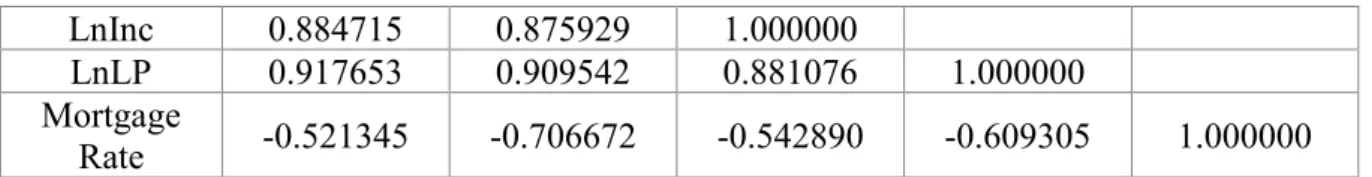
The behavior of house prices and economic fundamentals is illustrated by correlation analysis.
Variable LnGDP LnHP LnInc LnLP Mortgage Rate
LnGDP 1.000000 LnHP 0.896828 1.000000 100 113 131 145 145 138 89 72 0 50 100 150 200 250 300 350 2002 2003 2004 2005 2006 2007 2008 2009 2010 2011 2012 2013 2014 2015 2016 2017 California Shanghai
29
LnInc 0.884715 0.875929 1.000000
LnLP 0.917653 0.909542 0.881076 1.000000 Mortgage
Rate -0.521345 -0.706672 -0.542890 -0.609305 1.000000 Table 4. Correlation Matrix 2006Q1-2016Q3
Here and after, HP is average house price (yuan/sq m), Inc is per capita disposable income (yuan), LP is land price (yuan/sq m).
Table 4 displays the simple correlation among all variables during the period. The correlations between variables and house price were all strong over the period, and signs were as expected. House price had the lowest correlation of -0.7 with mortgage rate. Usually, when mortgage rate drops, the cost of buying a house decreases, and people would like to invest in the housing market, consequently leading to the higher demand and price of house. House price had the highest correlation of 0.9 with land price. As mentioned before, the land price
accounts for almost half of the house price, and the house price increases in-line with the land price. Besides, the increase of GDP and income have a positive impact on house prices as a strong economy and income improve affordability. Although correlation analysis indicates some intuition about the possible reasons for changes of house price, it is not enough to justify the existence of a bubble. Cointegration offers a better understanding of house price with fundamentals.
To detect cointegration, the order of integration of all variables should be tested. An ADF test is used with each variable in log form (except mortgage rate). The results in Table 5 suggest that variables (except income) are stationary after first differencing.
Variable
Level Result First difference Result
ADF value Critical value (5%) ADF value
Critical value (5%) LnHP -3.410069 -3.520787 N -9.022304 3.523623 - Y LnGDP -2.521562 -3.529758 N -22.17337 3.529758 - Y LnLP -2.339867 -3.520787 N -7.597333 -3.523623 Y LnInc -0.853247 -3.544284 N -3.168312 -3.544284 N Mortgage Rate -1.3853 -3.520787 N -4.81082 -3.523623 Y Table 5. ADF test of all variables
30
Next, we examine whether home prices and three variables (GDP, land price, and mortgage rate) are cointegrated (variable of disposable income is excluded in cointegration equations). Table 6 shows that 1 cointegration equation exists at 0.05 significance level, which suggested there might have been a long-term relationship between house price and the three economic fundamentals.
Data Trend: None None Linear Linear Quadratic
Test Type No Intercept Intercept Intercept Intercept Intercept
No Trend No Trend No Trend Trend Trend
Trace 1 2 1 1 1
Max-Eig 1 2 1 1 1
Table 6. Cointegration test 2006Q1-2016Q3
Selected (0.05 level) Number of Cointegrating Relations by Model Result from different methods:
Method Estimated Bubble Periods
Price-to-rent ratio 2008-2010, 2014-2016
Price-to-income ratio 2014-2016
Cointegation test Long-term relationship between 2006-2016 Based on the results of P-I and P-R ratios, housing prices increased substantially during 2008-2010, and there might have been a bubble during 2014-2016. In terms of the result of the cointegration test, house price changed in-line with the economic fundamentals in the long run and seemed to have no bubble. However, the result of the cointegration test might default due to a small sample, or there might have been a bubble in economic fundamentals, like the land price (land price increased by 200% from 2008 to 2009) in the model. Meanwhile, the price might deviate from the equilibrium in some period and was corrected later due to the change of market context. For instance, the house price increased during 2008-2010 because of the strong economy and lower mortgage rate; in the following year, policy was enforced to slow down the house market, and the price dropped. It is inferred that the Shanghai house market was inflated during 2008-2010 and that a bubble existed between 2014-2016.