The handle
http://hdl.handle.net/1887/18622
holds various files of this Leiden University
dissertation.
Author
: Vu, Van Thieu
Title
: Opportunities for performance optimization of applications through code
generation
Chapter 2
Automatic code generation for
Finite Element Methods applied
to the Shallow-Water equations
Currently, CTADEL can generate highly optimized Fortran code for several
schemes in weather forecast models such as dynamics [18], cloud [16], and tur-bulence [42]. All these codes use nite dierence methods for discretization.
In this chapter we describe how to extend CTADEL to generate code for the
energy conserving Galerkin nite element schemes. The advantage of nite dierences is that it can be very easy to implement. However, these meth-ods are restricted to handle rectangular shapes and simple alterations. With complex geometries and irregular physical structures, the use of nite element methods is more straightforward. Finite element methods are better suited for solving partial dierential equations over complicated domains. For instance, in the simulation of the weather pattern on the earth, it is more important to have accurate predictions over land than over the wide-open sea. In order to demonstrate that nite element methods can be incorporated into the HIRLAM frame work, we have chosen to take Galerkin nite element methods to solve the Shallow-Water equations [63] as an example. These equations describe a single homogenous layer of uid. In general they are applied to various problems, such as tidal ow, tsunamis in oceans, etc. In meteorology they are used to forecast the wind and geopotential, which is equivalent to pressure. Please note that although Galerkin nite element methods can be applied to irregular domain, in the context of its use in meteorology only regular domains are chosen in this chapter.
2.1
Galerkin finite element methods
This section gives a short description of Galerkin nite element methods for the Shallow-Water equations. For more details, the reader is referred to [72, 73, 75].
2.1.1
Galerkin projection and finite element methods
For an arbitrary eldφ, we assume the following representation ˜ φ(r) = N X ν=1 φνeν(r). (2.1)
Here rdenotes thexor y horizontal coordinates,eν are basis functions, N is a
degree andφν are coecients of approximation.
In order to formulate the nite element methods, it is necessary to approxi-mate a general eldφ(r)by a functionφ˜(r)in the form of the right hand side
of Equation (2.1). The transformation from φ(r) to φ˜(r) can be achieved by
the Galerkin projection as
˜
φ= (φν, eν), ν∈ {1,· · · , N}, (2.2)
where the scalar product (a, b)is computed as (a, b) =
Z
a(r)b(r)dµ, (2.3)
with
dµ=w(r)dxdy. (2.4)
The positive continuous function w is called the weight of the Galerkin
projection. The relation between the elds φ and φ˜, given by (2.2), can be
written as
˜
φ=Ghφi, (2.5)
where Gis called the Galerkin projection operator. The angle brackets denote
the Galerkin projection. For equations of the form
φt=f(φ), (2.6)
where the subscriptt denotes the dierentiation in time, the approximation ˜
φt=Ghf( ˜φ)i (2.7)
2.1. Galerkin finite element methods 11
2.1.2
The Galerkin finite element method for the
Shallow-Water equations
The Shallow-Water equations model the propagation of disturbances in water and other incompressible uids. The underlying assumption is that the depth of the uid is small compared to the wave length of the disturbance. The equations are derived from the principles of conservation of mass and conservation of momentum. The independent variables are time t, and two space coordinates x and y. The dependent variables are the uid height or depth H, and the two-dimensional uid velocity eld with components U and V in the x and y direction, respectively. With the proper choice of units, the conserved quantities are mass, which is proportional to H, and momentum, which is proportional to UH and VH. The force acting on the uid is gravity, represented by the gravitational constantg. The Shallow-Water equations have the following form
∂U ∂t =f V −U Ux−V Uy−gHx, ∂V ∂t =−f U−U Vx−V Vy−gHy, ∂H ∂t =−(U H)x−(V H)y, (2.8)
where the subscripts denote the dierentiation with respect to the specied variable, andf represents the Coriolis parameter, describing the rotation of the
earth.
The energy conserving scheme for the Shallow-Water equations, as proposed by Steppeler [73, 75, 74], reads as follows
∂U ∂t =G1 ηV − G2 1 2 U 2+V2 +gHx, ∂V ∂t =G1 D −ηU− G212 U2+V2+gHy E , ∂H ∂t =−G2 D (U H)x+ (V H)yE, η=Vx−Uy+f, (2.9)
whereηrepresents the absolute vorticity. G1andG2are the Galerkin operators with weights H and1, respectively.
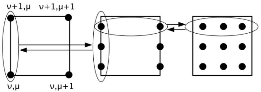
To approximate Equation (2.9) by the Galerkin nite element method, we interpolate the elds from the nodepoint to the y-collocation grid and then from the y-collocation to the collocation grid (see Figure 2.1). The purpose of interpolation is to create a ner resolution grid. Next, we compute the right hand side of Equation (2.9) on the collocation grid. Finally, we perform the
Figure 2.1: Nodepoint grid (left); y-collocation grid (middle), obtained by
interpolating the nodepoint grid in theydirection; and collocation grid (right), obtained by interpolating the y-collocation grid in the x direction. ν and µ are the coordinates of the nodepoint grid. Right arrow shows the interpolation. Left arrow shows the projection.
Galerkin projection in the xdirection and then in they direction to transform
from the collocation to the nodepoint grid. In the next paragraphs, we will describe these interpolations and projections.
Interpolation
Letξbe eitherxory andψ(ξ)be a function obtained from a two dimensional
function ψ(x, y) by keeping the other variable xed. Then, an interpolation
formula for an interval (a, b)can be written as
ψ(ξ) =ψ(a) (b−ξ) +ψ(b) (ξ−a)
b−a , (2.10)
where ψstands forU,V, or H. Within each interval, we always interpolate to
the three Gauss-pointsξρ,ρ= 1,2,3[1], dened as
ξρ= b−a 2 ξ 0 ρ+ b+a 2 , (2.11) with ξ10,3=∓ r 3 5, ξ20 = 0. (2.12)
Choosing the interval(a, b)≡(ξ, ξ+ 1)and substitute Equation (2.11) in
Equa-tion (2.10), we have
ψ(ξρ) =
ψ(ξ)1−ξ0ρ+ψ(ξ+ 1)1 +ξρ0
2.1. Galerkin finite element methods 13 Let ψ(ξ)+ =ψ(ξ) +ψ(ξ+ 1) 2 , 4+ψ(ξ) =ψ(ξ+ 1)−ψ(ξ) (2.14)
then Equation (2.13) can be rewritten as
ψ(ξρ) =ψ(ξ) + +1 2ξ 0 ρ4 +ψ(ξ). (2.15)
This equation is used for interpolation. With ξ =y and taking (ν, ν+ 1) as
interval, where ν is the coordinate in the x-direction of the nodepoint grid,
the interpolation will transform from the nodepoint to the y-collocation grid. Similarly, interpolation with ξ = x in the interval (µ, µ+ 1), where µ is the
coordinate in the y-direction of the nodepoint grid, will transform elds from
the y-collocation to the collocation grid (see Figure 2.1). Projection
Let RS(ξ) denote the right hand side of Equation (2.9) whereξ is eitherx or y. Then the Galerkin projection forRS(ξ)is dened as
GhRS(ξ)i= Z
eν(ξµ)RS(ξ)w(ξ)dξ, (2.16)
with basis functionseν(ξµ)dened by the properties
eν(ξµ) = 0, ifµ6=ν, 1, (2.17)
andw(ξ)is a weight function which is eitherH or1for theG1andG2Galerkin operator, respectively.
The integration of any functionψ(ξ)in the interval(a, b)can be computed
as follows Z b a ψ(ξ)dξ= 3 X ρ=1 ψ(ξρ)gρ(b−a), (2.18)
with ξρ are calculated according to Equation (2.11) andgρ are the
Gaussian-weights, dened as
g1,3= 0.55555555555,
g2= 0.88888888889.
Choosing the interval (a, b) ≡ (ξ, ξ+ 1) and substitute Equations (2.17) and (2.18) in Equation (2.16), we obtain ψ(ξ) = 4ξ 4 3 X ρ=1 ψ(ξρ)w(ξρ)gρ 1−ξρ0+ψ(ξρ−1)w(ξρ−1)gρ +ξ0ρψ(ξρ−1)w(ξρ−1)gρ . (2.20) Let ψ(ξρ)w(ξρ) − =ψ(ξρ−1)w(ξρ−1) +ψ(ξρ)w(ξρ) 2 (2.21) and 4−ψ(ξρ)w(ξρ) =ψ(ξρ)w(ξρ)−ψ(ξρ−1)w(ξρ−1), (2.22) we get ψ(ξ) = 4ξ 2 3 X ρ=1 gρ ψ(ξρ)w(ξρ) − −ξ 0 ρ 2 4 −ψ(ξ ρ)w(ξρ) . (2.23)
Equation (2.23) is used for projection. Ifξ=xand ψgiven on the
colloca-tion grid, by keeping y xed, the Galerkin projection will transform from the
collocation to the y-collocation grid. Similarly, if ξ=y and ψ is given on the
y-collocation grid, by keeping x xed, the Galerkin projection will transform
from the y-collocation to the nodepoint grid.
2.2
Specification
CTADELgenerates code from input specications. The problem, specied in a high-level language, is transformed into an Abstract Syntax Tree. Then com-mon subexpression elimination and architecture dependent optimizations are performed before the resulting code is generated. In this section we present
how to extend CTADELfor the Galerkin nite element methods. The Galerkin
nite element methods consist of two main steps: interpolation and projection. To simplify the implementation, we specify each step as a template. Next, we show the specication of the Shallow-Water equations applying the Galerkin nite element method.
2.2.1
Templates
Interpolation template
The interpolation of a eld is performed following Equation (2.15). In CTADEL
we dene the template interpolatewhich has as input ψ, the eld to be
inter-polated in the ξdirection, and as output the corresponding interpolated eld.
2.2. Specification 15
average_f(_::field Xi(grid),Xi) :: field Xi(half) average_f(Psi::float dim Unit,Xi) :: float dim Unit
:= 1/2*(Psi+Psi@(Xi=Xi+1)). delta_f(_::field Xi(grid) ,Xi) :: field Xi(half).
delta_f(Psi::float dim Unit,Xi) :: float dim Unit:=Psi@(Xi=Xi+1)-Psi. interpolate(_::field Xi(grid),_::field Xi(grid),Xi) ::field Xi(grid). interpolate(Psi::float dim Unit,Gp::float dim Unit,Xi)::float dim Unit
:= average_f(Psi,Xi)+1/2*Gp*delta_f(Psi,Xi).
In the templateinterpolate we denote average_f, delta_f, Psi, Gp, and Xi
for the notationsψ+,4+,ψ,ξ0, andξas in Equation (2.15), respectively. The LATEX output for this template produced by CTADELhas the following form
interpolateψ, ξ0ρ, ξ=ψ(ξ)++1 2ξ
0
ρ4
+ψ(ξ). (2.24)
We see that the right hand sides of Equations (2.15) and (2.24) are exactly the same. This proves that the templateinterpolate denition is correct.
Projection template
Based on Equation (2.23) we dene the templateprojectfor Galerkin projection.
This template has as input the eldψ(ξρ)to be projected in theξdirection, the
weight function w(ξρ), the Gauss-pointsξ
0
ρ and the Gauss-weightsgρ
parame-ters. The output ofprojectis the corresponding projected eld. The template projecthas the following form
average_b(_::field Xi(grid) ,Xi) :: field Xi(half). average_b(Psi::float dim Unit,Xi):: float dim Unit
:= 1/2*(Psi@(Xi=Xi-1)+Psi). delta_b(_::field Xi(grid) ,Xi) :: field Xi(half).
delta_b(Psi::float dim Unit,Xi) :: float dim Unit := Psi-Psi@(Xi=Xi-1). project(_::field Xi(grid),_::field Xi(grid),_::field Xi(grid),
_::field Xi(grid),Xi) :: field Xi(gird). project(Psi::float dim Unit,W::float dim Unit,Gp::float dim Unit,
Gw::float dim Unit,Xi)::float dim Unit := sum(1/2*delta(Xi)*Gw*(average_b((PsiW),Xi) -1/2*Gp*delta_b((PsiW),Xi)),rho = 1..3).
In the templateprojectaverage_b and delta_b denoteψ−and4−,
respec-tively, Psi is the input eldψ(ξρ), Xi is direction of projectionξ, W is the weight
gρ, respectively. CTADELproduces the LATEX output for this template as projectψ, w, ξ0ρ, gρ, ξ = 4ξ 2 P3 ρ=1 gρ ψ(ξρ)w(ξρ) − −ξ 0 ρ 24 −ψ(ξ ρ)w(ξρ) . (2.25)
The right hand side of Equation (2.25) is exactly the same as in Equation (2.23). This proves the correctness of the projecttemplate denition.
2.2.2
Specification of the Shallow-Water equations
We give the full specication of the Shallow-Water equations. The specication consists of the denitions of units and dimensions, the denitions of grids, and the discretization of the Shallow-Water equations. Note that in this chapter we
have chosen the rectangular grids. Based on this specication, CTADEL will
generates Fortran code.
Units and dimensions
At rst we need to dene all units and dimensions that are used for describing the Shallow-Water equations such as Distance (m), Time (s), Velocity (Dis-tance/Time), and Height (Distance). These units and dimensions are specied in CTADELas
% Define units and dimensions Distance : "m".
Time : "s".
[Velocity] :=[Distance]/[Time]. [Height] :=[Distance]. % Spatial variables
x ::float dim Distance. % for nodepoint grid y ::float dim Distance.
xc ::float dim Distance. % for collocation grid yc ::float dim Distance.
In the above specication, (x,y) and (xc,yc) are the spatial variables used to discretize elds on the nodepoint and the collocation grid, respectively.
Grids
Before dening the grids, we need to declare the grid sizes. The grid sizes, which are dened by L and LCOL for the nodepoint and collocation grid, respectively, are specied as
2.2. Specification 17
% Grid sizes
L ::natural. % for nodepoint grid LCOL ::natural. % for collocation grid
The grids that are used to discretize the Shallow-Water equations include the nodepoint, y-collocation, and collocation grid. The nodepoint grid has two dimension variables denoted aslongitudinalandlatitudinal. The y-collocation
grid is extended from the nodepoint grid by the sub-dimension denoted as
latit_collocation. The collocation grid is extended from the y-collocation grid
with the sub-dimension denoted as longi_collocation. In CTADEL the node-point, y-collocation, and collocation grids are specied as
% Define nodepoint grid
longitudinal :=i=1 .. L. latitudinal :=j=1 .. L.
nodepoint :=longitudinal by latitudinal. % Define y-collocation grid
latit_collocation :=jc=1 .. LCOL.
y_collocation :=nodepoint by latit_collocation. % Define collocation grid
longi_collocation :=ic=1 .. LCOL.
collocation :=y_collocation by longi_collocation.
The notation of a domain consists of a variable and an associated range of grid sizes. Specically, nodepoint denotes grid point (i,j) on a [1,L]×[1,L]
domain, y-collocation denotes grid point (i,j,jc) on a [1,L]×[1,L]×[1,LCOL]
do-main, and collocation denotes grid point (i,ic,j,jc) on a [1,L]×[1,LCOL]×[1,L]×
[1,LCOL] domain.
Discretization
Before discretizing the Shallow-Water equations by the Galerkin nite element method, we need to declare all parameters such as Coriolis F, Gauss-points Gp, and Gauss-weights Gw. These parameters are specied as
% Coriolis parameter F :: float dim "1/s".
% Gauss-points (Gp), Gauss-weights (Gw)
Gp::float field (xc(grid)) on longi_collocation. Gw::float field (xc(grid)) on longi_collocation.
Next we specify all inputs (U,V,H ), outputs (UT,VT,HT ) of the Shallow-Water equations, and intermediate values on the nodepoint, y-collocation, and
collocation grids. In the following specication, we denote the nodepoint, y-collocation, and collocation grid by node, ycol, andcol, respectively. For exam-plesUnode,Uycol, andUcolrepresent the eld U on the nodepoint, y-collocation, and collocation grid, respectively.
% Inputs U, V, and H are specified: % on nodepoint grid:
Unode::float dim Velocity field (x(grid),y(grid),t) on nodepoint.
Vnode::float dim Velocity field (x(grid),y(grid),t) on nodepoint.
Hnode::float dim Height field (x(grid),y(grid),t) on nodepoint.
% on y-collocation grid:
Uycol::float dim Velocity field (x(grid),y(grid),yc(grid),t) on y_collocation.
Vycol::float dim Velocity field (x(grid),y(grid),yc(grid),t) on y_collocation.
Hycol::float dim Height field (x(grid),y(grid),yc(grid),t) on y_collocation.
% on collocation grid:
Ucol ::float dim Velocity field (x(grid),xc(grid),y(grid),yc(grid),t) on collocation.
Vcol ::float dim Velocity field (x(grid),xc(grid),y(grid),yc(grid),t) on collocation.
Hcol ::float dim Height field (x(grid),xc(grid),y(grid),yc(grid),t) on collocation.
% Outputs UT, VT, and HT are specified: % on nodepoint grid:
UTnode::float dim Velocity field (x(grid),y(grid),t) on nodepoint.
VTnode::float dim Velocity field (x(grid),y(grid),t) on nodepoint.
HTnode::float dim Height field (x(grid),y(grid),t) on nodepoint.
% on y-collocation grid:
UTycol::float dim Velocity field (x(grid),y(grid),yc(grid),t) on y_collocation.
VTycol::float dim Velocity field (x(grid),y(grid),yc(grid),t) on y_collocation.
HTycol::float dim Height field (x(grid),y(grid),yc(grid),t) on y_collocation.
% on collocation grid:
UTcol ::float dim Velocity field (x(grid),xc(grid),y(grid),yc(grid),t) on collocation.
2.2. Specification 19
VTcol ::float dim Velocity field (x(grid),xc(grid),y(grid),yc(grid),t) on collocation.
HTcol ::float dim Height field (x(grid),xc(grid),y(grid),yc(grid),t) on collocation.
% Intermediate values UVH=G_2<1/2*(U^2+V^2)+gH> and XI are specified: % on nodepoint grid:
UVHnode::float dim Velocity field (x(grid),y(grid),t) on nodepoint.
% on y-collocation grid:
UVHycol::float dim Velocity field (x(grid),y(grid),yc(grid),t) on y_collocation.
% on collocation grid:
UVHcol ::float dim Velocity field (x(grid),xc(grid),y(grid),yc(grid),t) on collocation.
XIcol ::float dim Velocity field (x(grid),xc(grid),y(grid),yc(grid),t) on collocation.
We note that we solve the Shallow-Water equations in a number of time steps. Therefore, the above specication involves the time variable t.
The interpolate template dened in Subsection 2.2.1 is used to transform inputs from the nodepoint grid to the y-collocation and collocation grid. The interpolation of inputs are specied as
% Interpolate inputs from nodepoint to y-collocation. Uycol = interpolate(U,Gp,y).
Vycol = interpolate(V,Gp,y). Hycol = interpolate(H,Gp,y).
% Interpolate inputs from y-collocation to collocation grid. Ucol = interpolate(Uycol,Gp,x).
Vcol = interpolate(Vycol,Gp,x). Hcol = interpolate(Hycol,Gp,x).
We continue with the specication of the expressionG2h1 2 U
2+V2 +gHi,
which is used twice in the calculation ofU T andV T. For convenience, we denote
this expression byU V H. The specication ofU V H reads as % Compute expression: UVH = - G2<1/2*(U^2+V^2)+gH>
% Compute UVH on collocation grid UVHcol = -1/2*(Ucol^2+Vcol^2) - gHcol.
% Project UVH from collocation to the nodepoint grid
UVHycol = project_bound(UVHcol,1,Gp,Gw,x) if on x-boundary\\ project(UVHcol,1,Gp,Gw,x) otherwise.
UVH = project_bound(UVHycol,1,Gp,Gw,y) if on y-boundary\\ project(UVHycol,1,Gp,Gw,y) otherwise.
% Compute the derivative of UVH in the y-direction % (UVHycol_y = d(UVH)/dy) on the y_collocation grid % and interpolate it to collocation grid
UVHycol_y::float dim Velocity field (x(grid),y(grid),yc(grid),t) on y_collocation.
UVHcol_y::float dim Velocity field(x(grid),xc(grid),y(grid),yc(grid),t) on collocation.
UVHycol_y = d(UVH)/dy.
UVHcol_y = interpolate(UVHycol_y,Gp,x).
% Compute the derivative of UVH in the x-direction % (UVHcol_x = d(UVH)/dx) on the collocation grid
UVHcol_x::float dim Velocity field(x(grid),xc(grid),y(grid),yc(grid),t) on collocation.
UVHcol_x = d(UVHycol)/dx.
In the above specication, dX/dY stands for the derivative of variable X to variable Y. Its only use is where Y is a spatial variable. It is approximated by a nite dierence:
dX/dY =Xi+1−Xi
4Y , (2.26)
where4Y is the grid point distance inY direction,Xi andXi+1 denote values of X at grid pointi andi+ 1, respectively. Within CTADEL, Equation (2.26) is specied as:
d (_ :: field Y(grid)) / d (_ :: field Y(grid)) :: field Y(grid). d (X :: float dim Unit) / d (Y :: float dim Unit):: float dim Unit := (X @ (Y = Y+1) - X) / delta Y.
Finally, we specify the Shallow-Water equations on the collocation grid and the projection of the outputsU T,V T, andHT from the collocation grid to the
y-collocation and nodepoint grid as
% Compute outputs of the Shallow-Water equations on collocation grid UTcol = XI*Vcol + UVHcol_x.
VTcol = -XI*Ucol + UVHcol_y.
HTcol = -d(Ucol*Hcol)/dx - d(Vcol*Hcol)/dy. XI = d(Vcol)/dx - d(Ucol)/dy + F.
% Project outputs from collocation to y-collocation and nodepoint grid UTycol = project_bound(UTcol,H,Gp,Gw,x) if on x-boundary\\
project(UTcol,H,Gp,Gw,x) otherwise.
UT = project_bound(UTycol,H,Gp,Gw,y) if on y-boundary\\ project(UTycol,H,Gp,Gw,y) otherwise.
2.3. Generating code 21
VTycol = project_bound(VTcol,H,Gp,Gw,x) if on x-boundary\\ project(VTcol,H,Gp,Gw,x) otherwise.
VT = project_bound(VTycol,H,Gp,Gw,y) if on y-boundary\\ project(VTycol,H,Gp,Gw,y) otherwise.
HTycol = project_bound(HTcol,1,Gp,Gw,x) if on x-boundary\\ project(HTcol,1,Gp,Gw,x) otherwise.
HT = project_bound(HTycol,1,Gp,Gw,y) if on y-boundary\\ project(HTycol,1,Gp,Gw,y) otherwise.
2.3
Generating code
This section presents the code generation process in CTADEL. We describe the
steps that CTADEL performs in order to translate the abstract specication
to optimized Fortran code. We give the LATEX output of each step for the
eld H which is the result of the specication given in Subsection 2.2.2. These
LATEX outputs are produced by CTADELto compare the specication with the
mathematical description and to check the dierent steps. The outputs of the
elds U andV are similar.
In CTADEL, the code is generated through the following steps:
1. Get scalar values and dimensional analysis: All scalar values and equa-tions in the specication are retrieved and sorted in order of computation.
Then CTADEL analyzes all units and dimensions declared in the
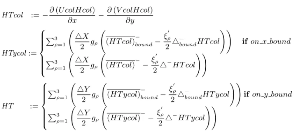
spec-ication. The result of this step is given in Figure 2.2. In this gure, Ucol, Vcol, and Hcol represent the interpolation values of U, V, and H on the collocation grid, respectively. HTcol, HTycol, and HT denote the interpolation values of the derivative in time of H (∂H/∂t) on the
collo-cation, y-collocollo-cation, and nodepoint grid, respectively. 4X and4Y are
the grid point distances on the nodepoint grid in the xand y direction,
respectively. In Figure 2.2, the rst equation shows the calculation of
HT on the collocation grid. Comparing to Equation 2.9, we conrm the
correctness of the Shallow-Water equations specication. The second and third equations show the projection of HT from the collocation grid to
the y-collocation and nodepoint grid, respectively. The projection at the boundary requires extra information. Hence, the boundary condition is included in the second and third equations.
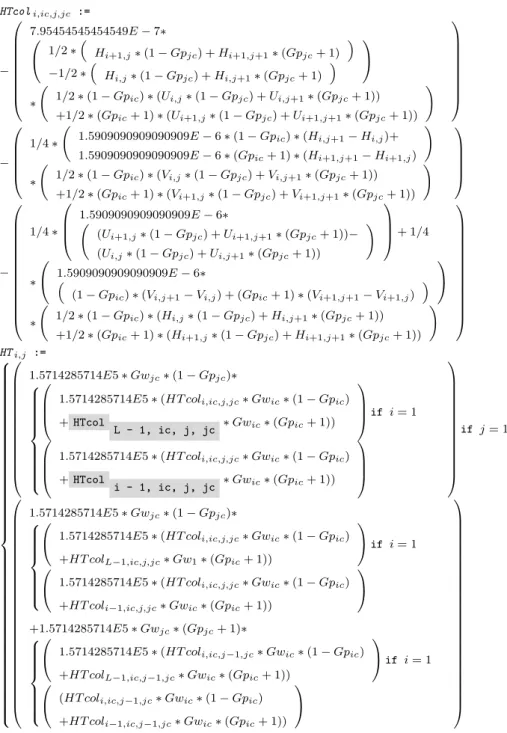
2. Discretization: Discretization of the continuous equations by the nite element method. Interpolation and Galerkin projection are used to dis-cretize all spatial variables and their derivatives. The output of this step consists of the spatial discrete equations as given in Figure 2.3. Since ex-tra information is needed for discretizing at the boundary, the boundary
HTcol :=−∂(U colHcol) ∂x − ∂(V colHcol) ∂y HTycol:= P3 ρ=1 4X 2 gρ (HT col) − bound− ξρ0 24 − boundHT col !! ifon x bound P3 ρ=1 4X 2 gρ (HT col) − −ξ 0 ρ 24 − HT col !! HT := P3 ρ=1 4Y 2 gρ (HT ycol) − bound− ξρ0 24 − boundHT ycol !! if on y bound P3 ρ=1 4Y 2 gρ (HT ycol) − −ξ 0 ρ 24 − HT ycol !!
Figure 2.2: LATEX output generated by CTADELafter get scalar values and dimensional analysis
condition is applied in this process. For example, the calculation ofHTi,j
needs the information of HT coli−1,ic,j,jc (shaded in Figure 2.3). Hence,
to calculateHT at the left boundary in thex-direction (i= 1), we need
the extra information ofHT col. Because we apply the periodic boundary
condition in the x-direction for the Shallow-Water equations, the value HT coli−1,ic,j,jcati= 1is replaced byHT colL−1,ic,j,jc. This example has
been marked by shading.
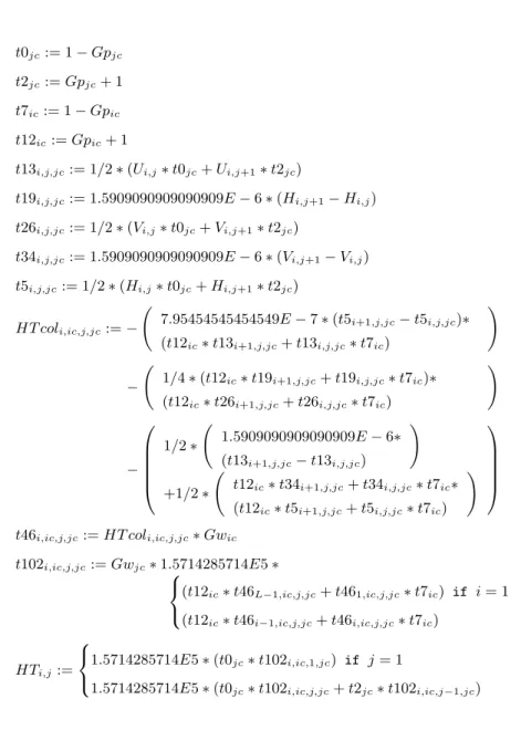
3. Common-subexpression elimination (CSE): The global CSE constructs a dataow graph for the intermediate code which is iteratively rened using a hardware cost model of the target computer architecture. The hardware cost model describes the relative cost of arithmetic and memory operations of the hardware resource. The result of CSE is an optimized intermediate code in which the subexpressions which are repeatly used are computed and stored in temporary variables for later usages. After CSE, CTADEL
gives the output as in Figure 2.4. In this gure, temporary variabes are denoted as t followed by a number. To compute HT, 11 temporary variables have been created. The use of temporary variables increases the eciency of computation. However, it results in the use of more memory.
4. Code generation: From the optimized intermediate code, CTADEL
pro-duces the Fortran code based on predened templates. The code generated by CTADEL is given in Figure 2.5. For brevity, we show only the code that relates to the calculations of HTcol and HT as in Figure 2.4.
2.3. Generating code 23 HTcoli,ic,j,jc := − 7.95454545454549E−7∗ 1/2∗ Hi+1,j∗(1−Gpjc) +Hi+1,j+1∗(Gpjc+ 1) −1/2∗ Hi,j∗(1−Gpjc) +Hi,j+1∗(Gpjc+ 1)
∗ 1/2∗(1−Gpic)∗(Ui,j∗(1−Gpjc) +Ui,j+1∗(Gpjc+ 1)) +1/2∗(Gpic+ 1)∗(Ui+1,j∗(1−Gpjc) +Ui+1,j+1∗(Gpjc+ 1)) ! −
1/4∗ 1.5909090909090909E−6∗(1−Gpic)∗(Hi,j+1−Hi,j)+ 1.5909090909090909E−6∗(Gpic+ 1)∗(Hi+1,j+1−Hi+1,j)
!
∗ 1/2∗(1−Gpic)∗(Vi,j∗(1−Gpjc) +Vi,j+1∗(Gpjc+ 1))
+1/2∗(Gpic+ 1)∗(Vi+1,j∗(1−Gpjc) +Vi+1,j+1∗(Gpjc+ 1)) ! − 1/4∗ 1.5909090909090909E−6∗ (Ui+1,j∗(1−Gpjc) +Ui+1,j+1∗(Gpjc+ 1))− (Ui,j∗(1−Gpjc) +Ui,j+1∗(Gpjc+ 1)) ! + 1/4 ∗ 1.5909090909090909E−6∗
(1−Gpic)∗(Vi,j+1−Vi,j) + (Gpic+ 1)∗(Vi+1,j+1−Vi+1,j)
∗ 1/2∗(1−Gpic)∗(Hi,j∗(1−Gpjc) +Hi,j+1∗(Gpjc+ 1)) +1/2∗(Gpic+ 1)∗(Hi+1,j∗(1−Gpjc) +Hi+1,j+1∗(Gpjc+ 1)) ! HTi,j := 1.5714285714E5∗Gwjc∗(1−Gpjc)∗
1.5714285714E5∗(HT coli,ic,j,jc∗Gwic∗(1−Gpic) +HTcol
L - 1, ic, j, jc ∗Gwic∗(Gpic+ 1))
if i= 1
1.5714285714E5∗(HT coli,ic,j,jc∗Gwic∗(1−Gpic) +HTcol
i - 1, ic, j, jc ∗Gwic∗(Gpic+ 1))
if j= 1 1.5714285714E5∗Gwjc∗(1−Gpjc)∗
1.5714285714E5∗(HT coli,ic,j,jc∗Gwic∗(1−Gpic) +HT colL−1,ic,j,jc∗Gw1∗(Gpic+ 1))
if i= 1
1.5714285714E5∗(HT coli,ic,j,jc∗Gwic∗(1−Gpic) +HT coli−1,ic,j,jc∗Gwic∗(Gpic+ 1))
+1.5714285714E5∗Gwjc∗(Gpjc+ 1)∗
1.5714285714E5∗(HT coli,ic,j−1,jc∗Gwic∗(1−Gpic) +HT colL−1,ic,j−1,jc∗Gwic∗(Gpic+ 1))
if i= 1
(HT coli,ic,j−1,jc∗Gwic∗(1−Gpic) +HT coli−1,ic,j−1,jc∗Gwic∗(Gpic+ 1))
Figure 2.3: LATEX output generated by CTADELafter discretization. The shading shows an example of applying the periodic boundary condition.
t0jc:= 1−Gpjc t2jc:=Gpjc+ 1 t7ic:= 1−Gpic t12ic:=Gpic+ 1
t13i,j,jc:= 1/2∗(Ui,j∗t0jc+Ui,j+1∗t2jc)
t19i,j,jc:= 1.5909090909090909E−6∗(Hi,j+1−Hi,j) t26i,j,jc:= 1/2∗(Vi,j∗t0jc+Vi,j+1∗t2jc)
t34i,j,jc:= 1.5909090909090909E−6∗(Vi,j+1−Vi,j) t5i,j,jc:= 1/2∗(Hi,j∗t0jc+Hi,j+1∗t2jc)
HT coli,ic,j,jc:=− 7.95454545454549E−7∗(t5i+1,j,jc−t5i,j,jc)∗ (t12ic∗t13i+1,j,jc+t13i,j,jc∗t7ic) ! − 1/4∗(t12ic∗t19i+1,j,jc+t19i,j,jc∗t7ic)∗ (t12ic∗t26i+1,j,jc+t26i,j,jc∗t7ic) ! − 1/2∗ 1.5909090909090909E−6∗ (t13i+1,j,jc−t13i,j,jc) ! +1/2∗ t12ic∗t34i+1,j,jc+t34i,j,jc∗t7ic∗ (t12ic∗t5i+1,j,jc+t5i,j,jc∗t7ic) !
t46i,ic,j,jc:=HT coli,ic,j,jc∗Gwic t102i,ic,j,jc:=Gwjc∗1.5714285714E5∗ (t12ic∗t46L−1,ic,j,jc+t461,ic,j,jc∗t7ic) if i= 1 (t12ic∗t46i−1,ic,j,jc+t46i,ic,j,jc∗t7ic) HTi,j:= 1.5714285714E5∗(t0jc∗t102i,ic,1,jc) if j= 1 1.5714285714E5∗(t0jc∗t102i,ic,j,jc+t2jc∗t102i,ic,j−1,jc)
2.3. Generating code 25 DO 119 jc=1,LCOL DO 120 j=0,L DO 121 ic=1,LCOL DO 122 i=0,L HTcol(i,ic,j,jc)=(-7.95454545454549E-7 *(t5(i+1,j,jc)-t5(i,j,jc))*(t12(ic) *t13(i+1,j,jc)+t13(i,j,jc)*t7(ic)))-2.5E-1 *(t12(ic)*t19(i+1,j,jc)+t19(i,j,jc)*t7(ic)) *(t12(ic)*t26(i+1,j,jc)+t26(i,j,jc) *t7(ic))-5.0E-1*(1.5909090909090909E-6 *(t13(i+1,j,jc)-t13(i,j,jc))+5.0E-1*(t12(ic) *t34(i+1,j,jc)+t34(i,j,jc)*t7(ic)))*(t12(ic) *t5(i+1,j,jc)+t5(i,j,jc)*t7(ic)) 122 CONTINUE * ENDDO 121 CONTINUE * ENDDO 120 CONTINUE * ENDDO 119 CONTINUE * ENDDO DO 147 j=1,L DO 148 i=1,L IF (0.EQ.1-j) THEN HT(i,j)=1.5714285714E5*(t0(jc)*t102(i,ic,1,jc)) ELSE HT(i,j)=1.5714285714E5*(t0(jc)*t102(i,ic,j,jc) +t102(i,ic,j-1,jc)*t2(jc)) ENDIF 148 CONTINUE * ENDDO 147 CONTINUE * ENDDO
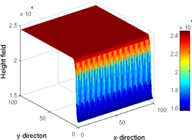
Figure 2.6: The Height field after 100 time steps
2.4
Experiments
The performance of the generated code is evaluated on an AMD 2.6 GHz Opteron with 4 GB RAM. The operating system is Scientic Linux 2.6.18. We compiled with gfortran 4.1.2 and Pathscale 3.0, both with the maximal optimization option (-O3).
The codes for the experiments are the hand-written code given in [75] and
the code generated by CTADELfor the Shallow-Water equations solved by the
Galerkin nite element method. The initial values were chosen the same as Steppeler [75], namely U =−1 f ∂H ∂y , V =−1 f ∂H ∂x, H =H0+H1tanh 9 (y−y0) 2D +H2 1 cosh2 9y −y0 D sin2πx, (2.27)
where H0= 20000, H1= 4400, H2 = 2660, and D = 4400000. The computa-tional domain consists of100×100 grid points. After 100 time steps, the eld
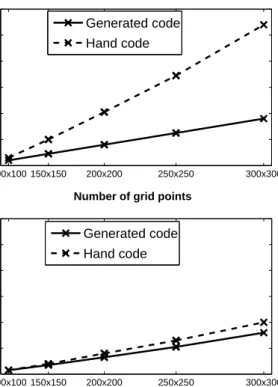
2.4. Experiments 27 100x100 150x150 200x200 250x250 300x300 20 40 60 80 100 120
Number of grid points
Execution time (s) Generated code Hand code 100x100 150x150 200x200 250x250 300x300 20 40 60 80 100 120
Number of grid points
Execution time (s)
Generated code Hand code
Figure 2.7: Execution times of the hand code and the generated code compiled
by the gfortran 4.1.2 (top) and the Pathscale 3.0 (down) compiler, both with -O3 optimization option
H looks like Figure 2.6.
We veried that the CTADELgenerated code reproduces the output of the
hand-written code within meteorological accuracy.
To compare the performance of the CTADELgenerated code with that of the hand code, we used a variety of domain sizes, and ran the model for each domain size during 100 time steps. Figure 2.7 shows the resulting execution times. We observe that both the hand code and the generated code scale very well with the number of grid points. The generated code is faster than the hand code, even strongly so for the gfortran compiled codes. This is mainly a consequence of the fact that the hand code in [75] is not well optimized, whereas CTADEL
performs optimizations like common subexpression elimination. Apparently, the Pathscale compiler optimizes the hand code rather better than gfortran, but for the generated code this eect is much less pronounced.
It should be mentioned that CTADELintroduces a large number of tempo-rary variables to store common subexpressions, and hence uses more memory, by an amount of 30%, than the hand code. This percentage can be reduced by re-using temporary variables, which feature CTADELis currently lacking.
2.5
Conclusions
Previous studies [18, 16, 43, 42] have shown that CTADELis able to generate ecient code for nite dierence methods. We have shown that the application
domain of CTADEL is not limited to nite dierence methods. As an
exam-ple, we applied it to the Galerkin nite element method for the Shallow-Water equations. Also for such a scheme it generates ecient (Fortran) code, that led to a faster executable than the original hand code. The speed gain depends on the compiler. It was close to a factor of 3 with an open source compiler. Furthermore, LATEX output, generated by CTADEL, provides a straightforward
means to verify that the model specication matches the modeller's intentions.
Currently, CTADEL is limited to rectangular grids, while a more complex
geometry mesh is usually required in nite element methods. Though mesh generation is an important component within nite element methods, we will not include mesh generation in CTADEL, instead, we limit CTADELto generate codes for grids produced by external mesh generators, because external mesh generators are highly optimized already for that purpose [23].