Robust, Scalable, and Provable Approaches to High Dimensional Unsupervised Learning

(1)

University of Central Florida University of Central Florida

STARS

Electronic Theses and Dissertations, 2004-2019

2018

Robust, Scalable, and Provable Approaches to High Dimensional

Unsupervised Learning

Mostafa Rahmani

University of Central Florida

Part of the Electrical and Computer Engineering Commons

Find similar works at: https://stars.library.ucf.edu/etd

University of Central Florida Libraries http://library.ucf.edu

This Doctoral Dissertation (Open Access) is brought to you for free and open access by STARS. It has been accepted for inclusion in Electronic Theses and Dissertations, 2004-2019 by an authorized administrator of STARS. For more information, please contact [email protected].

STARS Citation STARS Citation

Rahmani, Mostafa, "Robust, Scalable, and Provable Approaches to High Dimensional Unsupervised Learning" (2018). Electronic Theses and Dissertations, 2004-2019. 5818.

(2)

ROBUST, SCALABLE, AND PROVABLE APPROACHES TO HIGH DIMENSIONAL UNSUPERVISED LEARNING

by

MOSTAFA RAHMANI

M.S. Sharif University of Technology, 2012

A dissertation submitted in partial fulfilment of the requirements for the degree of Doctor of Philosophy

in the Department of Electrical and Computer Engineering in the College of Engineering and Computer Science

at the University of Central Florida Orlando, Florida

Spring Term 2018

(3)

(4)

ABSTRACT

This doctoral thesis focuses on three popular unsupervised learning problems: subspace clustering, robust PCA, and column sampling. For the subspace clustering problem, a new transformative idea is presented. The proposed approach, termed Innovation Pursuit, is a new geometrical solution to the subspace clustering problem whereby subspaces are identified based on their relative novelties. A detailed mathematical analysis is provided establishing sufficient conditions for the proposed method to correctly cluster the data points. The numerical simulations with both real and synthetic data demonstrate that Innovation Pursuit notably outperforms the state-of-the-art subspace cluster-ing algorithms. For the robust PCA problem, we focus on both the outlier detection and the matrix decomposition problems. For the outlier detection problem, we present a new algorithm, termed Coherence Pursuit, in addition to two scalable randomized frameworks for the implementation of outlier detection algorithms. The Coherence Pursuit method is the first provable and non-iterative robust PCA method which is provably robust to both unstructured and structured outliers. Coher-ence Pursuit is remarkably simple and it notably outperforms the existing methods in dealing with structured outliers. In the proposed randomized designs, we leverage the low dimensional structure of the low rank component to apply the robust PCA algorithm to a random sketch of the data as opposed to the full scale data. Importantly, it is analytically shown that the presented randomized designs can make the computation or sample complexity of the low rank matrix recovery algo-rithm independent of the size of the data. At the end, we focus on the column sampling problem. A new sampling tool, dubbed Spatial Random Sampling, is presented which performs the random sampling in the spatial domain. The most compelling feature of Spatial Random Sampling is that it is the first unsupervised column sampling method which preserves the spatial distribution of the data.

(5)

Dedicated to the memories of all the brave and hard working people who fought for dignity, justice, and freedom.

(6)

ACKNOWLEDGMENTS

I would like to sincerely thank my adviser, Dr. George Atia, for his assistance, support, and his trust in my research. I would also like to thank my mother, Nasrin Khodaveisi, and my wife, Sarah Shahraini, for their love and support. The research works presented in this thesis were supported in part by NSF CAREER Award CCF-1552497 and NSF Grant CCF-1320547.

(7)

LIST OF FIGURES

Figure 2.1: The subspace I(S2 ⊥ S1) is the innovation subspace of S2 over S1. The subspaceI(S2 ⊥ S1)is orthogonal toS1. . . 15

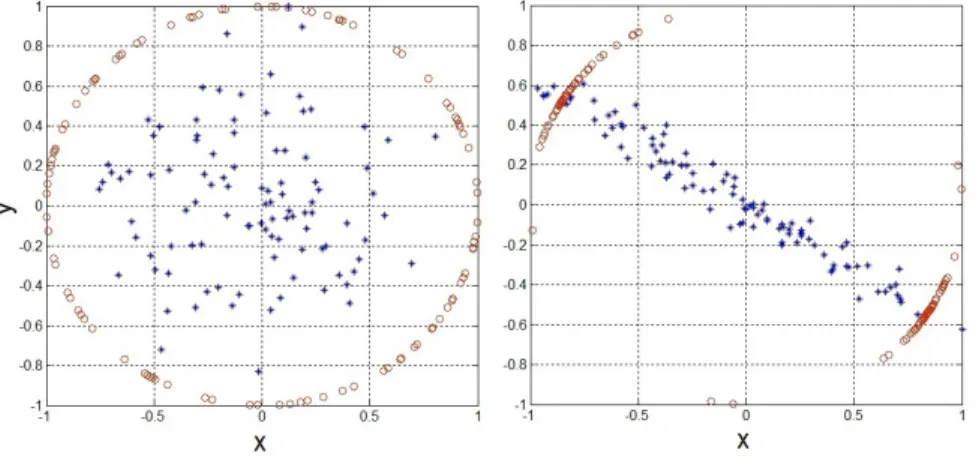
Figure 2.2: Data distributions in a two-dimensional subspace. The blue stars and red circles are the data points and their projections on the unit circle, respectively. In the left plot, the data points are distributed uniformly at random. Thus, they are not aligned along any specific directions and the permeance statistic cannot be small. In the right plot, the data points are aligned, hence the permeance statistic is small. . . 22

Figure 2.3: The left plot shows the output of (2.21), while the right plot shows the output of iPursuit when its search domain is restricted to the subspace spanned by the dominant singular vectors as per (2.22). . . 31

Figure 2.4: The output of the proposed method with different choices of the constraint vector. In the left and right plots, the first and the401th _{column are used as}

a constraint vector, respectively. The first column lies in a cluster with 100 data points and the401th column lies in a cluster with 6 data points. . . 35

Figure 2.5: The data lies in a union of 4 random 5-dimensional subspaces. In the left plot

N1 = 30. In the right plot,N1 = 10. For both plots, the first column is used as a constraint vector. . . 37

(17)

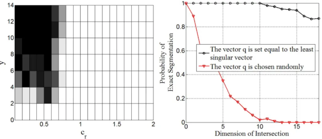
Figure 2.6: Left: Phase transition for various coherency parameters and dimension of the intersection. White designates exact subspace identification. Right: The performance of iPursuit (probability of exact segmentation) versus the di-mension of the intersection. . . 41

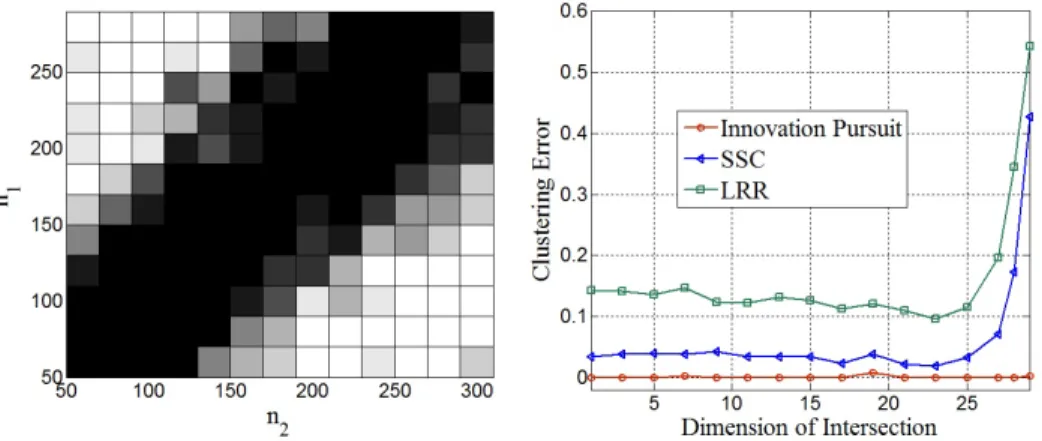
Figure 2.7: Left: Phase transition for different values of n1 andn2, the number of data points in the first and second subspaces. White designates exact subspace identification. Right: The clustering error of iPursuit, SSC and LRR versus the dimension of the intersection. . . 43

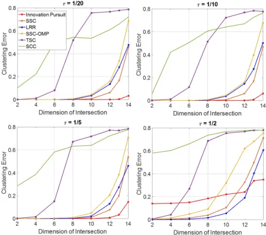
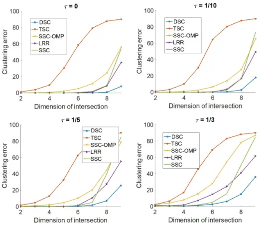
Figure 2.8: Performance of the algorithms versus the dimension of intersection for dif-ferent noise levels. . . 47

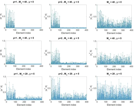
Figure 3.1: Measures of similarity|aT_X_|_and_|_xT

1X|adopted by DSC and TSC to identify a neighborhood set for the first data point. First rowM1 = 40and y = 0, second rowM1 = 40andy= 5, third rowM1 = 20andy= 5. . . 53

Figure 3.2: Performance of the algorithms versus the dimension of intersection for dif-ferent noise levels. . . 57

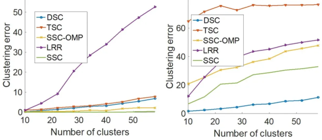
Figure 3.3: Performance with different number of data clusters. Left: the dimension of intersectiony= 0,Right: y= 4. . . 60

Figure 4.1: The values of vectorpfor different values ofpand ni

no. . . 70

(18)

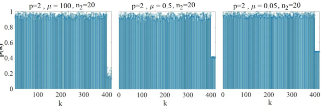
Figure 4.3: The data matrixD∈_R200×420_{contains 20 outliers and the distribution of the} outliers follows Assumption 4.2. The elements of the vectorpare shown for

different values of the parameterµ. . . 73

Figure 4.4: The functionlog₁₀f(t) = log₁₀ 1−I t N1 (0.5, N1/2−0.5) versustfor dif-ferent values ofN1, where I t N1 (0.5, N1/2−0.5)is the incomplete beta function. 80 Figure 4.5: The distribution of inliers withinU for different values of parameterνdefined in Assumption 4.4. If the value ofνincreases, the inliers are less clustered. . 84

Figure 4.6: The phase transition plot of exact subspace recoveru in presence of unstruc-tured outliers versusni/randno/m. . . 86

Figure 4.7: The subspace recovery error versusno/nifor unstructured outliers. . . 88

Figure 4.8: The first columns are the images obtained from the MSRA Salient Object Database. The second and third columns show the detection results obtained by CoP and FMS, respectively. . . 90

Figure 4.9: Some of the frames of the Waving Tree video file. The highlighted frames are detected as outliers by CoP and FMS. . . 90

Figure 4.10:The highlighted frames indicate the frames detected as outliers by R1-PCA. . 91

Figure 4.11:The clustering error after each iteration of Algorithm 7. . . 95

Figure 5.1: The rank ofΦLversusm2. . . 122

Figure 5.2: Phase transition plots of Algorithm 8 with RED. . . 126

(19)

Figure 5.4: Phase transition plots of Algorithm 8 with RED. . . 126

Figure 5.5: Phase transition plots of Algorithm 8 with RED (r = 20,ρ= 0.2). . . 127

Figure 5.6: Phase transition plot of Algorithm 9 with RED. . . 127

Figure 5.7: Phase transition plots of Algorithm 8 with both RED and RRD applied to motion tracking data. . . 128

Figure 5.8: A set of random examples of the faces in Yale database. . . 128

Figure 5.9: Random examples of the images in Caltech101 database. . . 128

Figure 5.10:The dimension ofUφandhversus the value ofm2. . . 129

Figure 6.1: Data distributions in a two-dimensional subspace. The red points are the normalized data points. . . 144

Figure 6.2: The rank of a set of uniformly sampled columns for different number of clus-ters. . . 145

Figure 6.3: Visualization of the matrices defined in Section 6. Matrix Dw is selected randomly or using Algorithm 12 described in Section 6. . . 148

(20)

Figure 6.4: Visualization of Algorithm 13. We run few cycles of the algorithm and stop when the rank of the LR component does not change over T consecutive steps. One cycle of the algorithm starts from the point marked “I” and pro-ceeds as follows. I: Matrix Dw is decomposed and Lˆw is the obtained LR

component ofDw. II: Algorithm 11 is applied toLˆw to select the

informa-tive columns of Lˆw. Lˆsw is the matrix of columns selected from Lˆw. III:

MatrixDcis formed from the columns ofD that correspond to the columns

ofLˆs

w. 1: MatrixDcis decomposed andLˆcis the obtained LR component of

Dc. 2: Algorithm 11 is applied toLˆTc to select the informative rows ofLˆc. Lˆsc

is the matrix of rows selected fromLˆc. 3: MatrixDw is formed as the rows

ofDcorresponding to the rows used to formLˆs_c. . . 158 Figure 6.5: Phase transition plots for various rank and sparsity levels. White designates

successful decomposition and black designates incorrect decomposition. . . . 163

Figure 6.6: Phase transition plots for various data matrix dimensions (r= 15, ρ= 0.05). 163

Figure 6.7: Performance of the proposed approach and the randomized algorithm in [1]. A value 1 indicates correct decomposition and a value 0 indicates incorrect decomposition. . . 165

Figure 6.8: Stationary background. . . 166

Figure 6.9: Two frames of a video taken in a lobby. The first column displays the original frames. The second and third columns display the LR and sparse components recovered using the proposed approach. . . 166

(21)

Figure 6.11:Performance of the proposed online approach and the online algorithm in [2]. 169

Figure 7.1: Left: The distribution of data in a two-dimensional space. The data consists of two clusters shown in yellow. The normalized points in the first and second clusters are distributed on two separate arcs with lengthsτ1 andτ2, respec-tively. Each of the two arcs does not overlap with the image of the other arc w.r.t. the origin on the unit circle. Right: The rank of randomly sampled columns by RIS and SRS versus the number of sampled columns. . . 176

Figure 7.2: The number of sampled columns from each data cluster for different values ofN1. . . 180

Figure 7.3: The number of columns sampled from each data cluster. In the left plot, the sampling algorithms are applied directly to the data. In the middle and right plot, the sampling algorithms are applied to a sketch of the data obtained through random embedding. . . 184

(22)

LIST OF TABLES

Table 2.1: Run time of different algorithms (N1 = 50,N = 3,{ri}3i=1 = 10,{ni}3i=1 = N2/3) . . . 44

Table 2.2: Run time of the different algorithms (r = 100, N1 = 110, N2 = 5000,

{ri}Ni=1 = 100/N,{ni}Ni=1 =N2/N) . . . 45

Table 2.3: Clustering error of innovation pursuit with coherent data . . . 47

Table 2.4: CE (%) of algorithms on Hopkins155 dataset (Mean - Median). . . 49

Table 3.1: Clustering error (%) of different algorithms on the Extended Yale B dataset. . 61

Table 4.1: Running time of the algorithms . . . 87

Table 4.2: Subspace recovery error, kU−UˆUˆT_U_k

F/kUkF, of the algorithms versus

the value of parameterµ. . . 93

Table 4.3: Average Clustering Error (ACE) of the algorithms for clustering the traffic data sequences with two motions (Mean - Median) . . . 94

Table 5.1: Order of sufficient number of random linear data observations. . . 102

Table 5.2: Run time of randomized Algorithm 9 with outlier detection and the Algo-rithm in [3]. . . 123

(23)

CHAPTER 1: INTRODUCTION AND NOTATION

Unsupervised learning is mainly concerned with discovering the hidden structure of data from the unlabeled data in which the data categorization is not included. The hidden and low-dimensional structures that prevail much of the data can yield representations that are more concise that the original observations. This succinct representation can be leveraged to compress the data, re-move/detect corruptions, filter out noise, and obtain a deep insight into the informational content of the data. This thesis focuses on three important unsupervised learning problems: robust PCA, subspace clustering, and data sampling. In the following sections, the structure of this thesis is out-lined and the new contributions of the presented research are summarized. At the end, the notation used throughout this thesis is presented.

Subspace Clustering

Linear subspace models are widely used in signal processing and data analysis since many datasets can be well approximated with low-dimensional subspaces. In many applications, the data is origi-nating from multiple independent sources, in which case a union of subspaces can accurately model the data. The problem of subspace clustering is concerned with learning these low-dimensional subspaces and clustering the data points to their respective subspaces. This problem arises in many applications, including computer vision (e.g. motion segmentation [4], face clustering [5]), gene expression analysis [6, 7], image processing [8], and system identification [9].

Many different approaches to subspace clustering were devised in related work, including statistical-based approaches [10–13], Spectral-Clustering [14], the algebraic-geometric approach [15], tive methods [16, 17], and Spectral-Clustering [18] based methods [14, 19–26]. The existing itera-tive methods either suffer from poor performance in presence of noisy data and close subspaces [4]

(24)

or their computational complexity grows exponentially with the number and the dimension of the subspaces [4]. In addition, the performance of existing Spectral-Clustering based methods de-grades when the intersection between the subspaces increases.

In Chapter 2 and Chapter 3, we focus on the subspace clustering problem and an entirely new approach, dubbed Innovation Pursuit, is presented. In the proposed approach, we introduce a new geometrical idea whereby subspaces are identified based on their relative innovations. We design two frameworks (an iterative and a Spectral-Clustering based framework) in which the idea of In-novation pursuit is used to distinguish the subspaces. The first framework, presented in Chapter 2, uses an iterative method that finds the subspaces consecutively by solving a series of simple linear optimization problems. Each linear optimization problem searches for a direction of innovation in the span of the data potentially orthogonal to all subspaces except for the one to be identified in one step of the algorithm. The proposed method can provably yield exact clustering even when the subspaces have significant intersections under mild conditions on the distribution of the data points in the subspaces. The second framework, presented in Chapter 3, integrates Innovation Pursuit with Spectral-Clustering to yield a new variant of Spectral-Clustering-based algorithms. The numerical simulations with both real and synthetic data demonstrate that Innovation Pursuit can often outperform the state-of-the-art subspace clustering algorithms, more so for subspaces with significant intersections, and that it notably advances the state-of-the-art result for subspace-segmentation-based face clustering.

The contributions of Innovation Pursuit

Innovation Pursuit advances the state-of-the-art research in subspace clustering on several fronts. Here we summarize the main contributions.

(25)

• The proposed approach introduces a new geometrical idea whereby the directions of inno-vation are utilized to distinguish the data clusters.

• The proposed iterative framework is the first scalable iterative algorithm with provable guar-antees. In contrast to the existing iterative methods whose complexity grows exponentioally with the number and dimension of subspaces and the Spectral-Clustering based methods whose complexity is quadratic or cubic in the number of data points, the computational complexity of the presented method only scales linearly in the number of subspaces and quadratically in their dimensions.

• The idea of innovation search enables the proposed methods to substantially outperform the existing segmentation algorithms in the challenging scenarios in which the dimensions of the intersections of the subspaces are large.

• The integration of the proposed innovation search optimization problem with Spectral-Clustering yields a new Spectral-Clustering based subspace segmentation method. We show through ex-tensive experiments with real and synthetic data that the presented Spectral-Clustering based method notably outperforms the existing Spectral Clustering based methods and yields the state-of-the-art result for the problem of face clustering using subspace segmentation.

Robust PCA (Subspace Recovery and Matrix Decomposition)

Principal Component Analysis (PCA) is arguably the most widely used data analysis tool for di-mensionality reduction. PCA is based upon a least-square optimization problem which finds the subspace whose `2-distance to the data points is minimal. However, the performance of PCA is notoriously sensitive to data corruptions and outliers. Specifically, in presence of data corruptions and outliers, the subspace obtained by PCA can arbitrarily deviate from the true underlying

(26)

sub-space. In the literature of the robust PCA problem, two main models for data corruption that are in fact incomparable for the most part are considered, the element-wise corruption and the column-wise corruption. In the element-column-wise model, the data corruption is modeled as a sparse matrix with arbitrary support which is added to the true data. In this model, the non-zero elements can affect all the columns/rows of the data. Under this corruption model, the robust PCA problem is known as the low rank plus sparse matrix decomposition problem. The second model is the column-wise model wherein only a fraction of the columns of the data are contaminated with the corruptions. These columns are called outliers and the objective is to detect them or obtain the span of the non-outlying columns (this problem is typically referred to as robust subspace recovery).

In this thesis, we investigate both corruption models and present new robust and scalable data recovery tools. In Chapter 4, a new provable robust (to outliers) PCA method, dubbed Coher-ent Pursuit, is presCoher-ented. In Chapter 5, two randomized designs are theoretically studied and it is shown that they provide a scalable framework for the implementation of outlier detection al-gorithms. In Chapter 6, we focus on the low rank plus sparse matrix decomposition problem in high-dimensional regimes and a randomized, provable, and scalable matrix decomposition method is proposed. In the following, we briefly review the presented research work on the robust PCA problem along with a summary of the new contributions.

Coherence Pursuit

Coherence Pursuit utilizes a new measure, termed Coherence value, to distinguish the outlying data points. The Coherence value is a measure of resemblance between a data point and the rest of data. Coherence Pursuit computes all the coherence values with a simple matrix multiplication and recovers the span of the inliers as the span of the data points with high coherence values. As Coherence Pursuit only involves one simple matrix multiplication, it is significantly faster than

(27)

the state-of-the-art robust PCA algorithms. We derive analytical performance guarantees for the proposed method under different models for the distributions of inliers and outliers in both noise-free and noisy settings. Coherence Pursuit is the first robust PCA algorithm that is simultaneously non-iterative, provably robust to both unstructured and structured outliers, and can tolerate a large number of unstructured outliers. The main contributions of the proposed approach can be summa-rized as follows:

• Coherence Pursuit employs a new measure to distinguish the outliers. The new measure enables the proposed method to accurately detect both structured and unstructured outliers.

• The proposed approach is the first robust (to outliers) PCA method which has performance guarantees with both structured and unstructured outliers.

• Coherence Pursuit is the first provably non-iterative outlier detection and subspace recovery method.

• The proposed approach can recover the true subspace even if the data is predominantly un-structured outliers and it notably outperforms the existing methods in detecting un-structured outliers.

Randomized outlier detection

In Chapter 5, we explore the robust (to outlier) PCA problem in high-dimensional regimes. We analyze two randomized designs in which low dimensional data sketches are processed to extract the data subspace. Both designs are shown to bring about substantial savings in complexity and memory requirements for robust subspace learning over conventional approaches that use the full scale data. The proposed randomized approach can provably recover the correct subspace with

(28)

computational and sample complexity that are almost independent of the size of the data. Some of the key technical contributions of the proposed randomized approach are listed below.

• In the first randomized design, the data sketch is formed by random column sampling fol-lowed by random low dimensional embedding. Somewhat surprisingly, it is shown that the sample complexity of the first randomized framework to guarantee exact subspace recovery is independent from the size of data.

• In the second randomized design, the data sketch is formed by random column sampling followed by random row sampling. For the second randomized design, it is proved that both the sample and computation complexities to guarantee exact subspace recovery are independent of the size of the data.

• The proposed randomized approach can provide a scalable framework for any outlier detec-tion algorithm.

High dimensional matrix decomposition

Conventional low rank plus sparse matrix decomposition algorithms use the entire data to extract the low-rank and sparse components, and are based on optimization problems whose complexity scales with the dimension of the data, which limits their scalability. In Chapter 6, we propose a scalable subspace-pursuit approach that transforms the decomposition problem to a low dimen-sional subspace learning problem. The decomposition is carried out using a small data sketch formed from sampled columns/rows. We provide performance guarantees with both random and adaptive column/row sampling. The key contributions of the proposed decomposition method are listed below.

(29)

• The proposed approach is based on a new randomized framework which extracts the low rank component in two consecutive steps. First, the column space of the low rank component is learned from a small subset of the columns of the data matrix. Second, the representation of the columns of the low rank matrix with respect to the learned column space is obtained from a small subset of the rows. If D ∈ _RN1×N2 _{is the given data, the decomposition}

complexity is reduced fromO(rN1N2)toO(max(N1, N2)r), whereris the rank of the low rank component.

• It is proved that even if we sample columns and rows uniformly at random, the sufficient number of sampled columns/rows to guarantee exact decomposition is linear with the rank and the coherence parameter of the low rank component.

• A new methodology for efficient column/row sampling is presented. The presented analy-sis shows that the proposed adaptive sampling procedure can make the required number of sampled columns/rows invariant to the data distribution.

• The proposed sequential column/row sampling method is the first scalable method for sam-pling from the highly structured/coherent data (in which both columns and rows follow clus-tering structures).

Spatially Random Column Sampling

Finding an informative or explanatory subset of a large number of data points is an important task of numerous machine learning and data analysis applications, including problems arising in com-puter vision [27], image processing [28], bioinformatics [29], and recommender systems [30]. The compact representation provided by the informative data points helps summarize the data, under-stand the underlying interactions, save memory, and enable remarkable computation speedups [31].

(30)

Over the last two decades, many different column sampling methods were proposed [32–34]. Most of these methods aim to find a small set of informative data columns whose span can well approxi-mate the given data. However, low rank approximation does not necessarily mean that the sampled data points represent the spatial distribution of the data. For instance, suppose the data points form multiple data clusters but the cluster centers are linearly dependent. The sampling algorithm which aims to preserve the column space of the data would not necessarily sample from each data cluster. Motivated by that, in Chapter 7 we introduce a novel randomized column sampling tool, dubbed Spatial Random Sampling (SRS), in which the random sampling is performed in the spatial do-main. SRS samples the data points based on their proximity to randomly sampled points on the unit sphere. The most compelling feature of SRS is that the corresponding probability of sampling from a given data cluster is proportional to the surface area the cluster occupies on the unit sphere, independently from the size of the cluster population. Although it is fully randomized, SRS is shown to provide descriptive and balanced data representations. The important contributions of the proposed sampling approach are listed below.

• SRS is the first unsupervised column sampling method which preserves the spatial distribu-tion of the data.

• If SRS is used for column sampling, the probability of sampling form a data cluster is inde-pendent of the cluster population size. Thus, SRS can obtain balanced data sketches from unbalanced data.

• The idea of random sampling in the spatial domain provides an entirely new data sketching tool. It addresses a pressing need in data science and holds potential to inspire many novel approaches for analysis of big data.

(31)

Notation

Bold-face upper-case letters are used to denote matrices and bold-face lower-case letters are used to denote vectors. Given a matrixA,kAkdenotes its spectral norm,kAk∗its nuclear norm,kAkF

its Frobenius norm, andcol(A) its column space. For a vectora, both kak and kak2 denote its `2-norm, a(i)itsith element, andkakp its`p-norm. For a matrixA, ai denotes its ith column, ai

its ith _row, _k_A_k

1,2 = P

ikaik2, and A−i is equal toA with the ith column removed. Given two

matricesA1 and A2 with equal number of rows, the matrix A3 = [A1 A2]is the matrix formed from the concatenation of A1 and A2. Given matrices {Ai}ni=1 with equal number of rows, we use the union symbol ∪ to define the matrix ∪n

i=1Ai = [A1 A2 ... An]as the concatenation of the matrices {Ai}ni=1. For a matrix D, we overload the set membership operator by using the notationd ∈ D to signify thatdis a column of D. A collection of subspaces {Gi}ni=1 is said to be independent if dim _n ⊕ i=1 Gi = Pn

i=1dim(Gi), where ⊕denotes the direct sum operator and

dim(Gi)is the dimension of Gi. Given a vector a,

a|is the vector whose elements are equal to the absolute value of the elements ofa. For a real numbera,sgn(a)is equal to1ifa > 0,−1if

a < 0, and0ifa= 0. The complement of a setLis denotedLc_{. Also, for any positive integer}_n_,

the index set{1, . . . , n}is denoted[n]. In addition,_SN1−1 _{denotes the unit}_`

2-norm sphere inRN1.

In an N-dimensional space, {ei}Ni=1 denotes the standard basis. The notationA = [ ]denotes an empty matrix.

(32)

CHAPTER 2: INNOVATION PURSUIT: A NEW GEOMETRICAL

SOLUTION FOR THE SUBSPACE CLUSTERING PROBLEM

In subspace clustering, a group of data points belonging to a union of subspaces are assigned membership to their respective subspaces. In this chapter1_{, we present our new approach, dubbed}

Innovation Pursuit (iPursuit), to the problem of subspace clustering using a new geometrical idea whereby subspaces are identified based on their relative novelties. The proposed approach finds the subspaces by solving a set of simple linear optimization problems, each searching for some direction of innovation in the span of the data that is potentially orthogonal to all subspaces ex-cept for the one to be identified in one step of the algorithm. A detailed mathematical analysis is provided establishing sufficient conditions for the proposed approach to correctly cluster the data points. The proposed approach can provably yield exact clustering even when the subspaces have significant intersections under mild conditions on the distribution of the data points in the sub-spaces. It is shown that the complexity of the proposed method scales only linearly in the number of data points and subspaces, and quadratically in the dimension of the subspaces. The numeri-cal simulations with both real and synthetic data demonstrate that iPursuit can often outperform the state-of-the-art subspace clustering algorithms, more so for subspaces with significant intersec-tions. Moreover, the proposed direction search approach can be integrated with Spectral-Clustering to yield a new variant of Spectral-Clustering-based algorithms. In this chapter, the iterative iPursuit algorithm is studied. In the next chapter, the Spectral-Clustering based framework is analyzed and it is shown that the integration of Innovation Pursuit with Spectral-Clustering yields the state of the art results for the challenging face clustering problem.

1_{The material presented in this chapter were partially published in the IEEE Transactions on Signal Processing and}

(33)

Introduction

The grand challenge of contemporary data analytics and machine learning lies in dealing with ever-increasing amounts of high-dimensional data from multiple sources and different modalities. The high-dimensionality of data increases the computational complexity and memory requirements of existing algorithms and can adversely degrade their performance [35]. However, the observa-tion that high-dimensional datasets often have intrinsic low-dimensional structures has enabled some noteworthy progress in analyzing such data. For instance, the high-dimensional digital facial images under different illumination were shown to approximately lie in a very low-dimensional subspace, which led to the development of efficient algorithms that leverage low-dimensional rep-resentations of such images [36, 37].

Linear subspace models are widely used in signal processing and data analysis since many datasets can be well-approximated with low-dimensional subspaces [38]. When data in a high-dimensional space lies in a single subspace, conventional techniques such as Principal Component Analysis (PCA) can be efficiently used to find the underlying low-dimensional subspace [39–41]. However, in many applications the data points may be originating from multiple independent sources, in which case a union of subspaces can better model the data [4].

The problem of subspace clustering is concerned with learning these low-dimensional subspaces and clustering the data points to their respective subspaces. This problem arises in many applica-tions, including computer vision (e.g. motion segmentation [4], face clustering [5]), gene expres-sion analysis [6, 7], and image processing [8]. Some of the difficulties associated with subspace clustering are that neither the number of subspaces nor their dimensions are known, in addition to the unknown membership of the data points to the subspaces.

(34)

Related work

Numerous approaches for subspace clustering have been studied in prior work, including statistical-based approaches [10], Spectral-Clustering [14], the algebraic-geometric approach [15] and itera-tive methods [16]. In this section, we briefly discuss some of the most popular existing approaches for subspace clustering. We refer the reader to [4] for a comprehensive survey on the topic. It-erative algorithms such as [16, 17] were some of the first methods addressing the multi-subspace learning problem. These algorithms alternate between assigning the data points to the identified subspaces and updating the subspaces. Some of the drawbacks of this class of algorithms is that they can converge to a local minimum and typically assume that the dimension of the subspaces and their number are known.

Another reputable idea for subspace segmentation is based on the algebraic geometric approach. These algorithms, such as the Generalized Principal Component Analysis (GPCA) [15], fit the data using a set of polynomials whose gradients at a point are orthogonal to the subspace containing that point. GPCA does not impose any restrictive conditions on the subspaces (they do not need to be independent), albeit it is sensitive to noise and has exponential complexity in the number of subspaces and their dimensions.

A class of clustering algorithms, termed statistical clustering methods, make some assumptions about the distribution of the data in the subspaces. For example, the iterative algorithm in [11, 12] assumes that the distribution of the data points in the subspaces is Gaussian. These algorithms typically require prior specifications for the number and dimensions of the subspaces, and are generally sensitive to initialization. Random sample consensus (RANSAC) is another iterative statistical method for robust model fitting [13], which recovers one subspace at a time by repeatedly sampling small subsets of data points and identifying a consensus set consisting of all the points in the entire dataset that belong to the subspace spanned by the selected points. The consensus set

(35)

is removed and the steps are repeated until all the subspaces are identified. The main drawback of this approach is scalability since the probability of selecting points belonging to the same subspace reduces exponentially with the number of subspaces. In turn, the number of trials required to select points in the same subspace grows exponentially with the number and dimension of the subspaces.

Much of the recent research work on subspace clustering is focused on Spectral-Clustering [18] based methods [14, 19–26]. These algorithms consist of two main steps and mostly differ in the first step. In the first step, a similarity matrix is constructed by finding a neighborhood for each data point, and in the second step Spectral-Clustering [18] is applied to the similarity matrix. Recently, several Spectral-Clustering based algorithms were proposed with both theoretical guarantees and superior empirical performance. The Sparse Subspace Clustering (SSC) [14], uses`1-minimization for neighborhood construction. In [23], it was shown that under certain conditions, SSC can yield exact clustering even for subspaces with intersection. Another algorithm called Low-Rank Rep-resentation (LRR) [22] uses nuclear norm minimization to find the neighborhoods (i.e., build the similarity matrix). LRR is robust to outliers but has provable guarantees only when the data is drawn from independent subspaces.

Contributions of proposed approach

The proposed approach, Innovation Pursuit, advances the state-of-the-art research in subspace clus-tering on several fronts. First, it rests on a novel geometrical idea whereby the subspaces are identified by searching the directions of innovation in the span of the data. Second, to the best of our knowledge iPursuit is the first scalable iterative algorithmwith provable guarantees – the computational complexity of iPursuit only scales linearly in the number of subspaces and quadrat-ically in their dimensions (c.f. Section 2). By contrast, GPCA [4,15] (without Spectral-Clustering) and RANSAC [13], which are popular iterative algorithms, have exponential complexity in the

(36)

number of subspaces and their dimensions. Third, innovation pursuit in the data span enables notably superior performance when the subspaces have considerable intersections. Fourth, the for-mulation enables many variants of the algorithm to inherit robustness properties in highly noisy settings (c.f. Section 2). Fifth, the proposed idea for direction search underlying iPursuit can be integrated with Spectral-Clustering to yield a new Spectral-Clustering based algorithm. The result-ing Spectral-Clusterresult-ing based method mostly outperforms the state-of-the-art Spectral-Clusterresult-ing based subspace segmentation methods and it yields the state-of-the-art result in the face clustering problem.

Proposed Approach

In this section, the core idea underlying iPursuit is described by first introducing a non-convex optimization problem. Then, we propose a convex relaxation and show that under mild sufficient conditions, solving the convex problem yields the correct subspaces. In this section (except for Section 2 on noisy data), it is assumed that the given data matrix follows the following data model.

Data Model 2.1. The data matrixD ∈ _RN1×N2 _{can be represented as} _D _{= [D}

1...DN]Twhere

T is an arbitrary permutation matrix. The columns of Di ∈ RN1×ni lie in Si, where Si is an

ri-dimensional linear subspace, for1≤i≤N, and,P_iN₌₁ni =N2. DefineVias an orthonormal

basis for Si. In addition, defineD as the space spanned by the data, i.e.,D = N

⊕

i=1

Si. Moreover,

it is assumed that any subspace in the set of subspaces{Si}Ni=1 has an innovation over the other

subspaces, to say that, for 1 ≤ i ≤ N, the subspace Si does not completely lie in N

⊕

k=1

k6=i

Sk . In

(37)

Innovation subspace

Consider two subspacesS1 andS2, such thatS1 6=S2, and one is not contained in the other. This means that each subspace carries some innovation w.r.t. the other. As such, corresponding to each subspace we define an innovation subspace, which is its novelty (innovation) relative to the other subspaces. More formally, the innovation subspace is defined as follows.

Definition 2.1. Assume that V1 andV2 are two orthonormal bases for S1 and S2, respectively.

We define the subspaceI(S2 ⊥ S1)as the innovation subspace ofS2 overS1 that is spanned by I−V1VT1

V2.In other words,I(S2 ⊥ S1)is the complement ofS1in the subspaceS1⊕ S2.

In a similar way, we can defineI(S1 ⊥ S2)as the innovation subspace ofS1overS2. The subspace

I(S1 ⊥ S2)is the complement ofS2inS1⊕S2. Fig. 2.1 illustrates a scenario in which the data lies in a two-dimensional subspaceS1, and a one-dimensional subspaceS2. The innovation subspace ofS2overS1is orthogonal toS1. SinceS1andS2are independent,S2andI(S2 ⊥ S1)have equal dimension. It is easy to see that the dimension of I(S2 ⊥ S1) is equal to the dimension of S2 minus the dimension ofS1∩ S2.

Figure 2.1: The subspace I(S2 ⊥ S1) is the innovation subspace of S2 over S1. The subspace

(38)

Innovation pursuit: Insight

iPursuit is a multi-step algorithm that identifies one subspace at a time. In each step, the data is clustered into two subspaces. One subspace is the identified subspace and the other one is the direct sum of the other subspaces. The data points of the identified subspace are removed and the algorithm is applied to the remaining data to find the next subspace. Accordingly, each step of the algorithm can be interpreted as a subspace clustering problem with two subspaces. Therefore, for ease of exposition we first investigate the two-subspace scenario then extend the result to multiple (more than two) subspaces. Thus, in this subsection, it is assumed that the data follows Data model 2.1 withN = 2.

To gain some intuition, we consider an example before stating our main result. Consider the case whereS1andS2are not orthogonal and assume thatn2 < n1. The non-orthogonality ofS1 andS2 is not a requirement, but is merely used herein to easily explain the idea underlying the proposed approach. Letc∗ be the optimal point of the following optimization problem

min ˆ c kˆc

T_D_k

0 s. t. cˆ∈ D and kcˆk= 1, (2.1)

wherek.k0 is the`0-norm. Hence,kcˆTDk0 is equal to the number of non-zero elements ofˆcTD. The first constraint forces the search for ˆc in the span of the data, and the equality constraint

kˆck = 1is used to avoid the trivialˆc = 0solution. Assume that the data points are distributed in

S1 andS2uniformly at random. Thus, the data is not aligned with any direction inS1andS2 with high probability (whp).

The optimization problem (2.1) searches for a non-zero vector in the span of the data that is or-thogonal to the maximum number of data points. We claim that the optimal point of (2.1) lies inI(S2 ⊥ S1)whp given the assumption that the number of data points inS1 is greater than the

(39)

number of data points inS2. In addition, since the feasible set of (2.1) is restricted toD, there is no feasible vector that is orthogonal to the whole data. To further clarify this argument, consider the following scenarios:

I. Ifc∗ lies inS1, then it cannot be orthogonal to most of the data points inS1 since the data is uniformly distributed in the subspaces. In addition, it cannot be orthogonal to the data points in S2 given thatS1 andS2 are not orthogonal. Therefore, the optimal point of (2.1) cannot be inS1given that the optimal vector should be orthogonal to the maximum number of data points. Similarly, the optimal point cannot lie inS2.

II. Ifc∗ lies inI(S1 ⊥ S2), then it is orthogonal to the data points inD2. However,n2 < n1. Thus, Ifc∗ lies inI(S2 ⊥ S1)(which is orthogonal toS1) the cost function of (2.1) can be decreased.

III. If c∗ lies in none of the subspaces S1, S2, I(S2 ⊥ S1) and I(S2 ⊥ S1), then it is not or-thogonal toS1 nor S2. Therefore,c∗ cannot be orthogonal to the maximum number of data points.

Therefore, the algorithm is likely to choose the optimal point from I(S2 ⊥ S1). Thus, if c∗ ∈

I(S2 ⊥ S1), we can obtainS2 from the span of the columns ofD corresponding to the non-zero elements of(c∗)T_D_{. The following lemma ensures that these columns span}_S

2.

Lemma 2.1. The columns ofDcorresponding to the non-zero elements of(c∗)T_D_span_S

2 if both

conditions below are satisfied:

i) c∗ ∈ I(S2 ⊥ S1).

ii) D2 cannot follow Data model 2.1 with N > 1, that is, the data points inD2 do not lie in

(40)

subspaces.

We note that if the second requirement of Lemma 2.1 is not satisfied, the columns of D2 follow Data model 2.1 withN ≥2, in which case the problem can be viewed as one of subspace clustering with more than two subspaces. The clustering problem with more than two subspaces will be addressed in Section 2.

Remark 2.1. At a high level, the innovation search optimization problem (2.1) finds the most sparse vector in the row space of D. Interestingly, finding the most sparse vector in a linear subspace has bearing on, and has been effectively used in, other machine learning problems, including dictionary learning and spectral estimation [42, 43]. In addition, it is interesting to note that in contrast to SSC which finds the most sparse vectors in the null space of the data, iPursuit searches for the most sparse vector in the row space of the data.

Convex relaxation

The cost function of (2.1) is non-convex and the combinatorial`0-norm minimization may not be computationally tractable. Since the`1-norm is known to provide an efficient convex approxima-tion of the`0-norm, we relax the non-convex cost function and rewrite (2.1) as

min ˆ c kˆc

T_D_k

1 s. t. cˆ∈ D and kcˆk= 1. (2.2)

The optimization problem (2.2) is still non-convex in view of the non-convexity of its feasible set. Therefore, we further substitute the equality constraint with a linear constraint and rewrite (2.2) as

(IP) min ˆ c kˆc

T_D_k

(41)

(IP) is the core program of iPursuit to find a direction of innovation. Here, q is a unit `2-norm vector which is not orthogonal toD. The vectorqcan be chosen as a random unit vector inD. In Section 2, we develop a methodology to learn a good choice forqfrom the given data matrix. The relaxation of the quadratic equality constraint to a linear constraint is a common technique in the literature [43].

Segmentation of two subspaces: Performance guarantees

Based on Lemma 2.1, to show that the proposed program (2.3) yields correct clustering, it suffices to show that the optimal point of (2.3) lies in I(S2 ⊥ S1) given that condition ii of Lemma 1 is satisfied, or lies in I(S1 ⊥ S2) given that condition ii of Lemma 1 is satisfied for D1. The following theorem provides sufficient conditions for the optimal point of (2.3) to lie inI(S2 ⊥ S1) provided that inf c∈I(S₂⊥S₁₎ cTq=1 kcTDk1 < inf c∈I(S₁⊥S₂₎ cTq=1 kcTDk1. (2.4)

If the inequality in (2.4) is reversed, then parallel sufficient conditions can be established for the optimal point of (2.3) to lie in the alternative subspaceI(S1 ⊥ S2). Hence, assumption (2.4) does not lead to any loss of generality.

Since I(S2 ⊥ S1)and I(S1 ⊥ S2) are orthogonal to S1 and S2, respectively, condition (2.4) is equivalent to inf c∈I(S₂⊥S₁₎ cTq=1 kcTD2k1 < inf c∈I(S₁⊥S₂₎ cTq=1 kcTD1k1. (2.5)

(42)

2 in the sense that it makes it more likely for the direction of innovation to lie inI(S2 ⊥ S1)2.

The sufficient conditions of Theorem 2.2 for the optimal point of (2.3) to lie in I(S2 ⊥ S1)are characterized in terms of the optimal solution to an oracle optimization problem (OP), where the feasible set of (IP) is replaced byI(S2 ⊥ S1). The oracle problem (OP) is defined as

(OP) min ˆ c kˆc T_D 2k1 subject to ˆc∈ I(S2 ⊥ S1) and ˆcTq= 1. (2.6)

Before we state the theorem, we also define the index setL0comprising the indices of the columns ofD2orthogonal toc2 (the optimal solution to (OP)),

L0 ={i∈[n2] :c2Tdi = 0,di ∈D2}, (2.7)

with cardinalityn0 =|L0|and a complement setLc0.

Theorem 2.2. Suppose the data matrixDfollows Data model 2.1 withN = 2. Also, assume that condition (2.5) and the requirement of Lemma 2.1 forD2 are satisfied (condition ii of Lemma 2.1).

Letc2 be the optimal point of the oracle program (OP) and define

α = X

di∈D2

sgn(cT₂di)di (2.8)

Also, letP2denote an orthonormal basis forI(S2 ⊥ S1),n0the cardinality ofL0defined in (2.7), 2_{Henceforth, when the two-subspace scenario is considered and (2.5) is satisfied, the innovation subspace refers to} I(S2⊥ S1).

(43)

and assume thatqis a unit`2-norm vector inDthat is not orthogonal toI(S2 ⊥ S1). If 1 2 δinf∈S₁ kδk=1 X di∈D1 δTd_i >kV₁TV₂k kαk+n0 , and kqTP2k 2kqT_V 1k inf δ∈S₁ kδk=1 X di∈D1 δTd_i ! >kVT₂P2k kαk+n0 , (2.9)

thenc2, which lies in I(S2 ⊥ S1), is the optimal point of (IP) in (2.3), and iPursuit clusters the

data correctly.

In what follows, we provide a detailed discussion of the significance of the sufficient conditions (2.9), which reveal some interesting facts about the properties of iPursuit.

1. The distribution of the data matters.

The LHS of (2.9) is known as the permeance statistic [41]. For a set of data pointsDiin a subspace

Si, the permeance statistic is defined as

P(Di,Si) = inf u∈S_i kuk=1 X di∈Di uTd_i . _(2.10)

The permeance statistic is an efficient measure of how well the data is distributed in the subspace. Fig. 2.2 illustrates two scenarios for the distribution of data in a two-dimensional subspace. In the left plot, the data points are distributed uniformly at random. In this case, the permeance statistic cannot be small since the data points are not concentrated along any directions. In the right plot, the data points are concentrated along some direction and hence the data is not well distributed in the subspace. In this case, we can find a direction along which the data has small projection.

Having n0 on the RHS underscores the relevance of the distribution of the data points within S2 since c2 cannot be simultaneously orthogonal to a large number of columns of D2 if the data does not align along particular directions. Hence, the distribution of the data points within each

(44)

subspace has bearing on the performance of iPursuit. We emphasize that the uniform distribution of the data points is not a requirement of the algorithm as shown in the numerical experiments. Rather, it is used in the proof of Theorem 2.2, which establishes sufficient conditions for correct subspace identification under uniform data distribution in worst case scenarios.

Figure 2.2: Data distributions in a two-dimensional subspace. The blue stars and red circles are the data points and their projections on the unit circle, respectively. In the left plot, the data points are distributed uniformly at random. Thus, they are not aligned along any specific directions and the permeance statistic cannot be small. In the right plot, the data points are aligned, hence the permeance statistic is small.

2. The coherency ofqwithI(S2 ⊥ S1)is an important factor.

An important performance factor in iPursuit is the coherency of the vector qwith the subspace

I(S2 ⊥ S1). To clarify, suppose that (2.5) is satisfied and assume that the vector q lies in D. If the optimal point of (2.3) lies in I(S2 ⊥ S1), iPursuit will yield exact clustering. However, if q is strongly coherent with S1 (i.e., the vector q has small projection on I(S2 ⊥ S1)), then the optimal point of (2.3) may not lie in I(S2 ⊥ S1). The rationale is that the Euclidean norm of any feasible point of (2.3) lying in I(S2 ⊥ S1) will have to be large to satisfy the equality

(45)

constraint whenqis incoherent withI(S2 ⊥ S1), which in turn would increase the cost function. As a matter of fact, the factor kqTP2k

kqT_V

1k in the second inequality of (2.9) confirms our intuition about

the importance of the coherency of qwithI(S2 ⊥ S1). In particular, (2.9) suggests that iPursuit could have more difficulty yielding correct clustering if the projection of q on the subspace S1 is increased (i.e., the projection of the vector on the subspace I(S2 ⊥ S1) is decreased). The coherence property could have a more serious effect on the performance of the algorithm for non-independent subspaces, especially when the dimension of their intersection is significant. For instance, consider the scenario where the vectorqis chosen randomly fromD, and defineyas the dimension of the intersection ofS1andS2. It follows thatI(S2 ⊥ S1)has dimensionr2−y. Thus,

EkqTP2k

E{kqTV1k}

= r2−y r1

. (2.11)

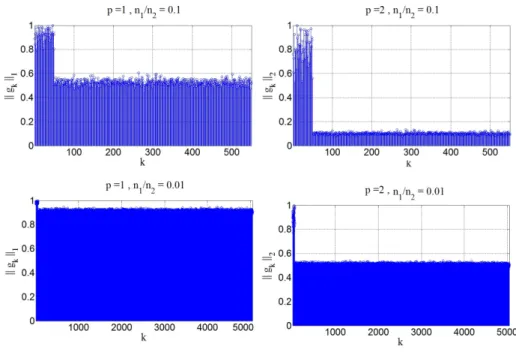
Therefore, a randomly chosen vectorqis likely to have a small projection on the innovation sub-space whenyis large. As such, in dealing with subspaces with significant intersection, it may not be favorable to choose the vector qat random. In Section 2 and section 2, we develop a simple technique to learn a good choice for q from the given data. This technique makes iPursuit re-markably powerful in dealing with subspaces with intersection as shown in the numerical results section.

Now, we demonstrate that the sufficient conditions (2.9) are not restrictive. The following lemma simplifies the sufficient conditions of Theorem 2.2 when the data points are randomly distributed in the subspaces. In this setting, we show that the conditions are naturally satisfied.

(46)

uni-formly at random from the intersection of the unit sphere_SN1−1_{and each subspace. If} r 2 π n1 r1 −2√n1−t1 r n1 r1−1 >2kVT₁V2k t2 √ n2−n0+n0 , kqT_P 2k kqT_V 1k r 2 π n1 r1 −2√n1−t1 r n1 r1−1 ! >2kV₂TP2k t2 √ n2−n0+n0 , (2.12)

then the optimal point of (2.3) lies inI(S2 ⊥ S1)with probability at least

1−exp−r2 2(t 2 2 −log(t22)−1) −exp −t 2 1 2 , for allt2 >1, t1 ≥0.

When the data does not align along any particular directions, n0 will be much smaller than n2 since the vector c2 can only be simultaneously orthogonal to a small number of the columns of D2. Noting that the LHS of (2.12) has ordern1 and the RHS has order

√

n2+n0 (which is much smaller than n2 whenn2 is sufficiently large), we see that the sufficient conditions are naturally satisfied when the data is well-distributed within the subspaces.

Clustering multiple subspaces

In this section, the performance guarantees provided in Theorem 2.2 are extended to more than two subspaces. iPursuit identifies the subspaces consecutively, i.e., one subspace is identified in each step. The data lying in the identified subspace is removed and optimal direction-search (2.3) is applied to the remaining data points to find the next subspace. This process is continued to find all the subspaces. In order to analyze iPursuit for the scenarios with more than two subspaces, it is helpful to define the concept of minimum innovation.

(47)

Definition 2.2. (Di,Si)is said to have minimum innovation w.r.t. the vectorqin the set{(Dj,Sj)}m_j₌₁ if and only if inf c∈I S_i⊥ m⊕ k=1 k6=i S_k cTq=1 kcTDik1 < inf c∈I S_j⊥ m⊕ k=1 k6=j S_k cTq=1 kcTDjk1 (2.13)

for everyj 6=i , 1≤j ≤m, whereqis a unit`2-norm in⊕mk=1Sk.

If(Dk,Sk)has minimum innovation in the set {(Dj,Sj)}N_j₌₁ (w.r.t. the vectorqused in the first

step), then we expect iPursuit to find Sk in the first step. Similar to Theorem 2.2, we make the

following assumption without loss of generality.

Assumption 2.1. Assume that(Dk,Sk)has minimum innovation w.r.t.qkin the set{(Dj,Sj)}k_j₌₁

for2≤k ≤N.

According to Assumption 2.1, ifqN is used in the first step as the linear constraint of the innovation

pursuit optimization problem, iPursuit is expected to first identifySN. In each step, the problem

is equivalent to disjoining two subspaces. In particular, in the (N −m+ 1)th step, the algorithm is expected to identifySm, which can be viewed as separating(Dm,Sm)and(

m−1 ∪ i=1Di , m−1 ⊕ i=1Si)by solving(IPm) (IPm) min ˆ c ˆ cT m∪ k=1Dk 1 subject to cˆ∈ ⊕m k=1 Sk , ˆcTqm = 1. (2.14) Note that ⊕m k=1

Sk is the span of the data points that have not been yet removed. Based on this

observation, we can readily state the following theorem, which provides sufficient conditions for iPursuit to successfully identifySm in the(N −m+ 1)

th

(48)

directly from Theorem 2.2 with two subspaces, namely, Sm and m−1

⊕

i=1Si. Similar to Theorem 2.2, the sufficient conditions are characterized in terms of the optimal solution to an oracle optimization problem (OPm)defined below.

(OPm) min ˆ c kˆc T_D mk1 subject to c∈ I Sm ⊥ m−1 ⊕ k=1Sk , ˆcTqm = 1. (2.15)

We also defineL0m = {i ∈ [nm] : cTmdi = 0, di ∈ Dm}with cardinalityn0m, wherecm is the

optimal point of (2.15).

Theorem 2.4. Suppose that the data follows Data model 2.1 withN = m and assume that Dm

cannot follow Data Model 2.1 withN > 1. Assume that(Dm,Sm)has minimum innovation with

respect toqm in the set{(Dj,Sj)}m_j₌₁. Definecm as the optimal point of(OPm)in (2.15) and let

αm =

P

di∈Dmsgn(c

T

mdi)di. Assumeqm is a unit`2-norm vector in

m ⊕ k=1 Sk. If 1 2_δ_∈minf−1 ⊕ k=1 S_k kδk=1 X di∈m∪−1 k=1Dk δTd_i >kV_mTT_m−1k kαmk+n0m , kqT mPmk 2kqT mTm−1k     inf δ∈m⊕−1 k=1 S_k kδk=1 X di∈m∪−1 k=1Dk δTdi     >kVT_mPmk kαmk+n0m , (2.16)

where Tm−1 is an orthonormal basis for

m−1

⊕

k=1

Sk and Pm is an orthonormal basis for I Sm ⊥ m−1

⊕

k=1

Sk

, thencm, which lies in I Sm ⊥ m−1

⊕

k=1

Sk

, is the optimal point of(IPm)in (2.14), i.e., the

subspaceSm is correctly identified.

(49)

Contrary to conventional wisdom, increasing the number of subspaces may improve the perfor-mance of iPursuit, for if the data points are well distributed in the subspaces, the LHS of (2.16) is more likely to dominate the RHS. In Chapter 8, we further investigate the sufficient conditions (2.16) and simplify the LHS to the permeance statistic.

Complexity analysis

In this section, we use an Alternating Direction Method of Multipliers (ADMM) [44] to develop an efficient algorithm for solving (IP). DefineU∈_RN1×r _{as an orthonormal basis for}D_{, where}_r

is the rank ofD. Thus, the optimization problem (2.3) is equivalent to

min a ka

T_UT_D_k

1 subject to aTUTq= 1.

Definef =UT_q_and_F₌_UT_D_{. Hence, this optimization problem is equivalent to}

min a,t ktk1+ µ 2kt−F T ak2+ µ 2(a T f −1)2 subject to t=FTa , aTf = 1, (2.17)

with a regularization parameterµ. The Lagrangian function of (2.17) can be written as

L(t,a,y1, y2) =ktk1+ µ 2kF T_a₋_t_k2₊µ 2(a T_f ₋₁₎2₊_yT 1(F T_a₋_{t) +}_y 2(aTf −1), (2.18)

where y1 and y2 are the Lagrange multipliers. The ADMM approach uses an iterative pro-cedure. Define (ak,tk) as the optimization variables and (yk1, y2k) the Lagrange multipliers at the kth _{iteration. Define} _G _:= _µ−1_(FFT ₊ _ffT₎−1 _{and the element-wise function} _T

(x) :=

(50)

1. Obtainakby minimizing the Lagrangian function with respect toawhile the other variables are

held constant. The optimalais obtained as

ak+1 =G µFtk−Fyk1 +f(µ−y k 2) . 2. Similarly, updatetas tk+1 =Tµ−1(FTa_k₊₁+µ−1yk₁).

3. Update the Lagrange multipliers as follows

y1 =y1+µ(FTak+1−tk+1) , yk2+1 =y

k

2 +µ(a

T_f ₋₁₎_.

These 3 steps are repeated until the algorithm converges or the number of iterations exceeds a predefined threshold. The complexity of the initialization step of the solver is O(r3) plus the complexity of obtainingU. Obtaining an appropriateUhasO(r2N2)complexity by applying the clustering algorithm to a random subset of the rows ofD(with the rank of sampled rows equal tor). In addition, the complexity of each iteration of the solver isO(rN2). Thus, the overall complexity is less thanO((r3₊_r2_N

2)N)since the number of data points remaining keeps decreasing over the iterations. In most cases,r N2, hence the overall complexity is roughlyO(r2N2N).

iPursuit brings about substantial speedups over most existing algorithms due to the following: i) Unlike existing iterative algorithms (such as RANSAC) which have exponential complexity in the number and dimension of subspaces, the complexity of iPursuit is linear in the number of subspaces and quadratic in their dimension. In addition, while iPursuit has linear complexity in

(51)

step plus the complexity of obtaining the similarity matrix, ii) More importantly, the solver of the proposed optimization problem hasO(rN2)complexity per iteration, while the other operations – whose complexity areO(r2N2)andO(r3)– sit outside of the iterative solver. This feature makes the proposed method notably faster than most existing algorithms which solve high-dimensional optimization problems. For instance, solving the optimization problem of the SSC algorithm has roughlyO(N3

2 +rN2)complexity per iteration [14].

How to choose the vectorq?

The previous analysis revealed that the coherency of the vector q with the innovation subspace is a key performance factor for iPursuit. While our investigations have shown that the proposed algorithm performs very well when the subspaces are independent even when the vectorqis chosen at random, randomly choosing the vector q may not be favorable when the dimension of their intersection is increased (c.f. Section 2). This motivates the methodology described next that aims to identify a “good” choice of the vectorq.

Consider the following least-squares optimization problem,

min ˆ q kqˆ

T_D_k

2 s. t. qˆ ∈ D and kqˆk= 1. (2.19)

The optimization problem (2.19) searches for a vector in D that has a small projection on the columns ofD. The optimal point of (2.19) has a closed-form solution, namely, the singular vector corresponding to the least non-zero singular value of D. When the subspaces are close to each other, the optimal point of (2.19) is very close to the innovation subspace I(S2 ⊥ S1). This is due to the fact that I(S2 ⊥ S1) is orthogonal to S1, hence a vector in the innovation subspace will have a small projection on S2. As such, when the subspaces are close to each other, the

(52)

least singular vector is coherent with the innovation subspace and can be a good candidate for the vector q. In the numerical results section, it is shown that this choice of q leads to substantial improvement in performance compared to using a randomly generatedq. However, in settings in which the singular values ofDdecay rapidly and the data is noisy we may not be able to obtain an exact estimate ofr. This may lead to the undesirable usage of a singular vector corresponding to noise as the constraint vector. In the next section, we investigate stability issues and present robust variants of the algorithm in the presence of noise. We remark that with real data or when the data is noisy, by the least singular vector we refer tothe least dominantsingular vector and not to the one corresponding to the smallest singular value which is surely associated with the noise component.

Noisy data

In the presence of additive noise, we model the data as

De =D+E, (2.20)

whereDeis the noisy data matrix,Dthe clean data which follows Data model 2.1 andEthe noise

component. The rank ofDis equal tor. Thus, the singular values ofDecan be divided into two

subsets: the dominant singular values (the first r singular values) and the small singular values (or the singular values corresponding to the noise component). Consider the optimization problem (IP) usingDe, i.e.,

min ˆ c kˆc

T_D

ek1 s.t. ˆc∈span(De) and cˆTq= 1. (2.21)

Clearly, the optimal point of (2.21) is very close to the subspace spanned by the singular vectors corresponding to the small singular values. Thus, ifcedenotes the optimal solution of (2.21), then