Kernel Density Estimation of Reliability With Applications to Extreme Value Distribution

(1)

University of South Florida

Scholar Commons

Graduate Theses and Dissertations Graduate School

10-16-2008

Kernel Density Estimation of Reliability With

Applications to Extreme Value Distribution

Branko Miladinovic

University of South Florida

Follow this and additional works at:https://scholarcommons.usf.edu/etd Part of theAmerican Studies Commons

This Dissertation is brought to you for free and open access by the Graduate School at Scholar Commons. It has been accepted for inclusion in Graduate Theses and Dissertations by an authorized administrator of Scholar Commons. For more information, please contact

Scholar Commons Citation

Miladinovic, Branko, "Kernel Density Estimation of Reliability With Applications to Extreme Value Distribution" (2008).Graduate Theses and Dissertations.

(2)

Kernel Density Estimation of Reliability With Applications to Extreme Value Distribution

by

Branko Miladinovic

A dissertation submitted in partial fulfillment of the requirements for the degree of

Doctor of Philosophy

Department of Mathematics & Statistics College of Arts and Sciences

University of South Florida

Major Professor: Chris P. Tsokos, Ph.D. Gangaram Ladde, Ph.D.

Kandethody Ramachandran, Ph.D. Marcus McWaters, Ph.D.

Date of Approval: October 16, 2008

Keywords: Gumbel, Bayesian, optimal bandwidth, target time, unbiased estimation c

(3)

Dedication

To my father Stanisav Miladinovic, who introduced me to Mathematics and whose love made all of this possible

(4)

Acknowledgements

My deepest appreciation goes out to my major professor and mentor Professor Chris Tsokos for his help and encouragement during my study. His advice and ex-pertise in the field of Statistics have shown me the merits of academic research. I would like to express my gratitude to Professors Kandethody Ramachandran, Gan-garam Ladde, and Marcus McWaters for their service on my dissertation committee. I would like to thank Professor Edward Mierzejowski for chairing my dissertation committee. Lastly, I would like to acknowledge late Professor A.N.V. Rao for his ad-vice during the course of my study, and above all for being an example of a wonderful human being.

(5)

Table of Contents

List of Figures . . . iv

List of Tables . . . vi

Abstract . . . ix

1 Introduction . . . 1

1.1 Basic Properties of the Reliability Function . . . 1

1.2 Justification for Bayesian Analysis . . . 4

1.3 The Gumbel Failure Model . . . 5

1.4 The Nonparametric Kernel Density Estimate of Reliability . 8 1.5 Contents of the Present Study . . . 11

2 The Kernels: An Evaluation . . . 13

2.1 Introduction . . . 13

2.2 Kernels and Their Properties . . . 14

2.3 Evaluation of Kernel Effectiveness in Density Estimation . . 19

2.4 New Ranking Based on Differences in Optimal Bandwidth for PDF, CDF, and Reliability Functions . . . 22

Visual Inspection Procedure to Determine Optimal Bandwidth for CDF and Reliability Functions . . . 24

2.5 Bandwidth Robustness . . . 29

2.6 Conclusion . . . 33

3 Ordinary, Bayes, Empirical Bayes, and Kernel Density Reliability Estimates for the Gumbel Failure Model . . . 34

(6)

3.3 Reliability Modeling . . . 37

3.4 Bayes Estimators of Reliability . . . 40

Lindley Approximation of ˆhB(t) . . . 43

3.5 Non-parametric Kernel Density Estimates of Reliability . . . 47

3.6 Numerical Results . . . 48

4 Sensitivity Behavior of Bayesian Reliability for the Gumbel Failure Model for Different Priors . . . 60

4.2 The Priors . . . 61

4.3 Main Results . . . 66

Properties of Reliability . . . 70

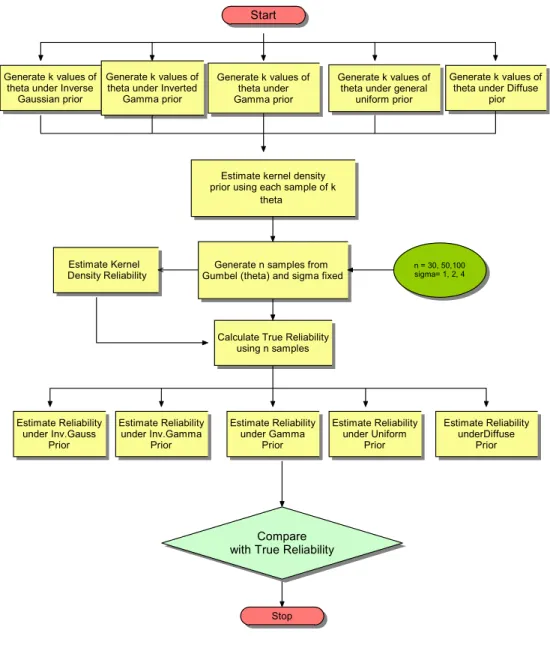
4.4 Numerical Comparison of Priors . . . 71

5 Bayesian Modeling of Target Time for the Gumbel Failure Model: Random Location and Scale Parameters . . . 74

5.2 The Gumbel Model . . . 74

5.3 Reliability Modeling . . . 75

5.4 Bayesian Approach to the Gumbel Model . . . 76

Jeffrey’s Non-informative Prior . . . 76

Posterior Distribution . . . 77

Bayesian Estimation of tα for Jeffrey’s Prior . . . 78

The Lindley Approximation . . . 79

5.5 Numerical Analysis . . . 82

6 The Choice of the Loss Function Under Bayesian Parameter Estimation 87 6.1 Introduction . . . 87

(7)

Criterion 1: Minimax Criterion Using Posterior Risks . . . 88

Criterion 2: Makov’s Criterion . . . 88

Criterion 3: Goodness of Fit Criterion . . . 89

Criterion 4: Probability Density Criterion . . . 89

6.3 Main Results . . . 90

Criterion 1: Minimax Criterion Using Posterior Risks . . . 92

Criterion 2: Makov’s Criterion . . . 93

Criterion 3: Goodness of Fit Criterion . . . 94

Criterion 4: Probability Density Criterion . . . 94

6.4 Criteria Comparison . . . 95

7 Kernel Density Estimation as an Alternative to the Gumbel Distribution in Modeling Quantiles and Return Periods for Flood Prevention . . . . 102

7.2 Preliminary Exploration of the Extreme Stream Flow Data . 104 7.3 Peak Stream Flow Quantile and Return Period Modeling . . 106

Model 1: The Maximum Likelihood Model . . . 109

Models 2 and 3: Time Dependent Location Parameter . . . 112

Model 4: The Jackknife Model . . . 114

Model 5: A Bayesian Model . . . 116

Model 6: The Non-parametric Kernel Density Model . . . 118

7.4 Model Comparison and Recommendation . . . 121

8 Future Research . . . 127

References . . . 129

Appendices . . . 138 About the Author . . . End Page

(8)

List of Figures 2.1 Epanechnikov Kernel . . . 15 2.2 Cosine Kernel . . . 15 2.3 Biweight Kernel . . . 16 2.4 Triweight Kernel . . . 16 2.5 Gaussian Kernel . . . 17 2.6 Triangle Kernel . . . 17 2.7 Uniform Kernel . . . 18

2.8 Numerical Study of Kernel Ranking . . . 27

3.1 Gamma Prior for α = 5, β = 0.5 . . . 50

3.2 Gamma Prior for α = 5, β = 1 . . . 50

3.3 Gamma Prior for α = 5, β = 4 . . . 51

3.4 Optimal Reliability for h=0.4286 . . . 52

3.5 Numerical Study of Gumbel Reliability . . . 53

4.1 Numerical Study of Priors . . . 65

5.1 Numerical Study of the Gumbel Failure Time . . . 84

6.1 Goodness of Fit Criterion Implementation Chart . . . 95

6.2 Kernel Density Criterion Implementation Chart . . . 96

7.1 Annual Maxima Stream Flow for the Hillsborough River 1940-2006 105 7.2 Ninety-five Percent Confidence Band Frequency Factor Plot for the Annual Peak Stream Flow . . . 107

(9)

7.3 Stream Flow Quantile Function Under the ML Estimates with 95 % Confidence Bands . . . 111 7.4 Stream Flow Return Period Function Under ML . . . 112 7.5 Stream Flow Quantile Function Under Jackknife . . . 116 7.6 Stream Flow Return Period Function Under the Jackknife Model 116 7.7 Stream Flow Quantile function Under Jackknife and Bayes Models 118 7.8 Return Period Function Under Jackknife, Bayes, and Kernel Density

(10)

List of Tables

1.1 Most Commonly Used Kernels . . . 9

2.1 Kernels and Their Inefficiencies . . . 21

2.2 Rate of Decrease of AMISE For All Seven Kernels as a Function of Sample Size . . . 21

2.3 Mean Integrated Square Error (MISE) for the Top Three Bandwidths for Data From Gumbel (n=15, 30, 50, 100, 200, σ = 1 ) . . . . 28

2.6 AMISE Rate of Change for h∗_{, n = 20 . . . .} ₃₁

2.7 AMISE Rate of Change for h∗_{, n = 50 . . . .} ₃₁

2.8 AMISE Rate of Change for h∗_{, n = 100 . . . .} ₃₂

3.1 Generated θ Values Under the Gamma Prior With α = 5, β = 0.5 49 3.2 Generated θ Values Under the Gamma Prior With α = 5, β = 1 49 3.3 Generated θ Values Under the Gamma Prior With α = 5, β = 4 49 3.4 MISE for the Reliability Estimates . . . 55

3.5 MISE for the Failure Rate Function Estimates . . . 56

3.6 MISE for the Cumulative Failure Function Estimates . . . 57

3.7 MISE for the Target Time tc . . . 58

(11)

4.2 MISE Under Inverted Gamma Prior . . . 68

4.3 MISE Under Gamma Prior . . . 68

4.4 MISE Under General Uniform Prior . . . 69

4.5 MISE Under Diffuse Prior . . . 70

4.6 Average Integrated Mean Square Errors for σ = 1 . . . 72

5.1 Comparison Between ML and Bayesian Estimates of Reliability Time: µ _∼ N(25, 1), σ = 1,2,4, α = 0.01 . . . 84

6.1 Prior Parameter Values . . . 97

6.2 Percentage of Success of the Different Criteria . . . 97

6.3 Numerical Comparison of the Different Criteria Used for the Choice of the Loss Function . . . 100

7.1 ML Estimates of the Location and Shape Parameter Estimates and Goodness of Fit . . . 111

7.2 Log-likelihood Estimates for ML Linear and Quadratic Trend Mod-els . . . 113

7.3 Location and Shape Parameter Estimates Under the Jackknife Model and Goodness of Fit . . . 115

7.4 Goodness of Fit P-values for the Kernel Density Method for the Top Kernel and Optimal Bandwidth . . . 120

7.5 Differences Between the Empirical, and Jackknife, Bayes, and Kernel Density CDF Estimates for the Top Eight Tail Values . . . 121

(12)

7.6 Major Quantiles for the Annual Peak Stream Flow Under the Top Four Models . . . 122 7.7 Hillsborough River Annual Peak Stream Flow Near Zephyrhills, FL. 126

(13)

Kernel Density Estimation of Reliability with Applications to Extreme Value Distribution

Branko Miladinovic

Abstract

In the present study, we investigate kernel density estimation (KDE) and its appli-cation to the Gumbel probability distribution. We introduce the basic concepts of reliability analysis and estimation in ordinary and Bayesian settings. The robustness of top three kernels used in KDE with respect to three different optimal bandwidths is presented. The parametric, Bayesian, and empirical Bayes estimates of the reli-ability, failure rate, and cumulative failure rate functions under the Gumbel failure model are derived and compared with the kernel density estimates. We also introduce the concept of target time subject to obtaining a specified reliability. A comparison of the Bayes estimates of the Gumbel reliability function under six different priors, including kernel density prior, is performed. A comparison of the maximum likeli-hood (ML) and Bayes estimates of the target time under desired reliability using the Jeffrey’s non-informative prior and square error loss function is studied. In order to determine which of the two different loss functions provides a better estimate of the location parameter for the Gumbel probability distribution, we study the perfor-mance of four criteria, including the non-parametric kernel density criterion. Finally, we apply both KDE and the Gumbel probability distribution in modeling the annual extreme stream flow of the Hillsborough River, FL. We use the jackknife procedure to improve ML parameter estimates. We model quantile and return period functions both parametrically and using KDE, and show that KDE provides a better fit in the tails.

(14)

1 Introduction

In the present study, we will investigate non-parametric kernel density estimation and its application to an extreme value distribution, namely the Gumbel probability distribution. The primary objective is to introduce non-parametric kernel density methodology, in order to estimate the probability density function of given data when we cannot identify a classical probability density function. The subject non-parametric kernel density is a function of two important quantities, namely the kernel function and the optimal bandwidth. We will evaluate seven most commonly used kernels and rank the top three with respect to their effectiveness, which will be mea-sured by the size of the mean square error (MSE), in conjuction with a selected optimal bandwidth. This methodology will be applied to reliability analysis when we cannot identify the failure probability density function of a given system. We will show that this non-parametric statistical procedure is quite effective when compared to parametric analysis. We proceed to introduce some preliminary definitions and procedures that will be used in the present study.

1.1 Basic Properties of the Reliability Function

Let T1, T2,...,Tn be a random sample of size n taken from a population of interest,

where T1, T2,...,Tn are independent and identically distributed. A complete

charac-terization of the random variable being observed is given only if we can specify exactly its probability distribution function. A function with values f(t), defined over the set of all real numbers, is called a probability density function (PDF) of the continuous

(15)

random variable T if and only if

P(a_≤T _≤b) = Z b

a

f(t)dt (1.1.1)

for any real constants a and b with a_≤b. A function can serve as a probability density of a continuous random variable T if its values, f(t), satisfy the conditions

f(t)_≥0, _{−∞ ≤}t_≤+_∞ (1.1.2) and

Z +∞

−∞

f(t)dt= 1 (1.1.3)

The function F(t) = P(T _≤ t) is called the cumulative distribution function (CDF) of the random variable T. If T denotes the time to failure of a particular system from time 0 to time t, then the reliability function R(t) is the probability that a system will be operable up to time t and is defined as

R(t) =P(T > t) = 1₋F(t) = Z ∞

t

f(x)dx (1.1.4) where f(t) is the probability density function of the random variable T. The values R(t) of the reliability function of a random variable T satisfy the conditions:

R(0) = 1 and R(+_∞) = 0 (1.1.5) and

if a < b, then R(a)_≥R(b) (1.1.6) for any real numbers a and b. In reliability analysis, one is interested in estimating the time at which a given system will fail. By solving for the quantile tα for which

(16)

we obtain the expression which for a given system represents the ”target time” to failure tα with at least (1 - α)100% confidence. Also related to reliability are the

failure rate and cumulative failure rate functions. The failure rate function, h(t), is the probability that a given system will fail for the first time after time t, given that it has operated up to time t. Under the reliability function R(t), the definitions of the failure rate function h(t) and cumulative failure rate function, H(t), are given respectively by h(t) = − ∂R(t) ∂t R(t) (1.1.8) and H(t) =₋ln(R(t)) (1.1.9) When engaged in reliability analysis, given T1, T2,...,Tn failure times, we first proceed

through goodness-of-fit tests and possibly filtering methods to identify parameters of a classical well defined probability density function that probabilistically character-izes the behavior of failure times. Only if we are not able to identify such a density function, we proceed non-parametrically. The problems of reliability for a specified probability distribution have received a great deal of attention in the past years. It has been of particular interest to obtain a minimum variance unbiased (MVU) esti-mator of reliability due to considerable cumulative effects of bias in complex systems. For instance, Pugh (1964) obtained MVU estimates of reliability for the exponen-tial failure model. Tate (1959) and Basu (1964) derived MVU estimators of the scale parameter and the reliability function for the exponential, Weibull, and Gamma probability distribution functions. Glasser (1962) derived MVU estimators for the Poisson probability distribution. The MVU estimators were derived by using func-tions of complete and sufficient statistics, as shall we in our study. Our main focus will be on the Gumbel failure model in ordinary and Bayesian settings, so we proceed to discuss Bayesian methodology next.

(17)

1.2 Justification for Bayesian Analysis

Bayesian inference procedures have gained wide spread popularity in recent years; however, justification is seldom given when such procedures are used by scientists and engineers. Bayesian analysis rests on the idea that if a scientist performs an experiment, new statistical inferences can be built upon earlier understanding of a phenomenon under study. It also provides a methodology to formally combine that earlier understanding with currently measured data, so that it updates the degree of belief (subjective probability) of the experimenter. The earlier understanding is called the ”prior belief,” which is the understanding held prior to observing the cur-rent set of data, available from the experimenter or other sources. The new belief, which results from updating the prior information, is called the ”posterior belief.” This is the new updated understanding held after having observed the current data, examined in light of how well they conform with preconceived notions. If we feel con-fident that the prior information derived from earlier experiments may improve our reliability estimates when performing reliability analysis, then Bayesian methodology is more appropriate. If we assume that parameters within failure models behave as random variables individually or jointly following certain distributions, we may use Bayesian analysis, which exploits a suitable prior information and the choice of a loss function in association with Bayes’ Theorem. The theorem shows us that to find subjective probability for some event or unknown quantity, we need to multiply our prior beliefs about the event by an appropriate summary of the observational data. This assumption may well be justified. Through experimentation we may notice that due to the complexity of electronic and structural systems, undetected component interactions resulting in unpredictable fluctuations of the parameters are present. To a reliability engineer this approach would seem to be appealing because it provides for the formulation of a distributional form for an unknown parameter based on the prior convictions or available information, especially as reliability prediction techniques are based on pooled and organized experience of countless individuals and organization. Another type of Bayesian analysis, introduced by Robbins (1980), involves estimating

(18)

a parameter of a data distribution without knowing or assessing the parameters of the subjective prior probability distribution. This analysis, called empirical Bayes, esti-mates the prior distribution of a parameter directly from the data. In our study we will engage in both classical and empirical Bayes analysis. Crelin (1972), Drake (1966), and Evans (1969) give excellent philosophical justifications for the use of Bayesian methodologies in reliability analysis. Tsokos (1972) gave an excellent review of the Bayesian approach to reliability and clearly expressed the usefulness of Monte Carlo simulation. Cavanos and Tsokos (1970) introduced the concept of empirical Bayes approach to reliability for the Weibull failure model. Cavanos and Tsokos (1971) derived classical and empirical Bayes estimates for the parameter and reliability for the Gamma failure model, along with Monte Carlo numerical study to illustrate the sensitivity of the estimates. Because the philosophy behind empirical Bayes estima-tion rests on the assumpestima-tion that the existence of a prior distribuestima-tion is known, but its form is unknown, our study will involve both classical Bayes and empirical Bayes methodologies, as well as Monte Carlo simulation, to illustrate the usefulness of our estimates. In our study the main focus will be on the Gumbel failure model, which we discuss next.

1.3 The Gumbel Failure Model

From probability theory, for the largest number of n independent identically dis-tributed random variables Y1, Y2, ..., Yn, i.e.,

X :=max(Y1, Y2, ..., Yn)

the probability distribution function is given by Mn(x) = [F(x)]n

where F(x) = P(Yi ≤ x) is the common probability distribution function of each

(19)

not constant but rather can be regarded as a realization of a random variable with Poisson probability distribution with mean ν, then the distribution of X becomes (e.g. Todorovic and Zelenhasic, 1970; Rossi et al., 1984),

M_ν′(x) =exp_{−ν(1₋F(x))_}

Since ln [F(x)]n _{≈ −}_n₍₁₋_F₍_x_{)) , it follows that for large n or large F(x),} _M

n(x) ≈

M′

n(x). Gumbel (1958), following the pioneering works by Frchet (1927), Fisher and

Tippet (1928) and Gnedenco (1941), developed a comprehensive theory of extreme value distributions. That is, as n tends to infinity, Mn(x) converges to one of three

possible asymptotic distributions, depending on the mathematical form of F(x). Ob-viously, the same limiting distributions may also result from Mν(x) as ν tends to

infinity. All three asymptotic distributions can be described by a single mathematical expression introduced by Jenkinson (1955, 1969) known as the Generalized Extreme Value (GEV) probability distribution function. This expression is given by

M(x) = exp_{−(1 + k(x−µ) σ )

−1/k

}, kx _≥kµ₋σ (1.3.1) where µ, σ > 0 and k are location, scale and shape parameters, respectively. When k = 0, the type I probability distribution of maxima (EV1 or Gumbel distribution) is obtained as a special case of the GEV distribution. Using simple calculus it is found that in this case, the cumulative distribution function takes the form

M(x) =exp(₋exp(₋x−µ

σ )) (1.3.2)

which is unbounded from both left and right. Therefore, for a sample of n random iid failure times, T1, T2,...,Tn, the reliability function under the Gumbel failure model

is given by

R(t) = 1₋exp(₋exp(₋t−µ

σ )) (1.3.3)

(20)

Incidentally, when k > 0, M(x) represents the extreme value probability distribution of maxima of type II (EV2). In this case the variable is bounded from the left and unbounded from the right (µ-σ/k = x < _∞). A special case is obtained when the left bound becomes zero (σ = kµ). This special two-parameter distribution has been known as the Frchet distribution and has the simplified form

M(x) =exp(₋(µ x)

1/k₎_{, x}

≥0

with µ becoming a scale parameter. Since the GEV probability distribution involves three parameters, it always provides better estimates than the Gumbel probability distribution; however, practically, it is also more difficult to work with due to the ana-lytic constraints involved in three versus two parameter estimation, as two parameters are more accurately estimated than three. Due to its simplicity and generality, the Gumbel probability has been introduced as a failure model for reliability studies. A recent book by Kotz and Nadarajah (2000) lists over 50 application ranging from accelerated life testing through to earthquakes, floods, horse racing, rainfall, queues in supermarkets, sea currents, wind speeds, and track race records. In particular, the Gumbel probability distribution has been used to characterize real world problems for several reasons. Most types of parent probability distributions functions that are used in reliability, such as exponential, Gamma, Weibull, normal, lognormal (Kottegoda and Rosso (1997)) belong to the domain of attraction of the Gumbel distribution. In contrast, the domain of attraction of the GEV distribution includes less commonly met parent probability distributions like Pareto, Cauchy, and log-gamma. Developed in the 1950’s, goodness-of-fit probability plots are the most common tools used by practitioners and engineers to choose an appropriate distribution function. EV1 offers a linear Gumbel probability plot, which is estimated in terms of plotting positions, i.e. sample estimates of probability of non-failure. In contrast, a linear probability plot for the three-parameter GEV is not possible to construct. This may be regarded as a primary reason of choosing EV1 against the three-parameter GEV in practice, assuming that two parameters produce results almost as good as three. For the

(21)

for-mer case, mean and standard deviation (or second L-moment) suffice, whereas in the latter case the skewness is also required and its estimation is extremely uncertain for typical small-size reliability samples. However, EV1 has one disadvantage, which is very important from the engineering point of view: for small probabilities of failure or exceedence it yields the smallest possible quantiles in comparison to those of the three-parameter GEV for any (positive) value of the shape parameter k. This means that EV1 results in the highest possible risk for engineering structures (Farquharson et al. (1992), Turcotte (1994), Turcotte and Malamud (2003)). We will establish in chapter 7 that kernel density estimation provides an alternate and relatively easy way to remedy this potential drawback of the Gumbel probability distribution. As stated earlier, if we are not able to identify the underlying probability density function for a given data set parametrically, we may do so non-parametrically. We proceed to introduce non-parametric kernel density estimation as a powerful alternative.

1.4 The Nonparametric Kernel Density Estimate of Reliability

The main problem with the parametric approach is that existing classical probability distribution families are limited in the face of a multitude of data structures. A wrong assumption concerning the underlying distribution model for the data may lead to misleading interpretations. In situations such as these, non-parametric methods may be more suitable. The nonparametric methods impose only mild assumptions, such as smoothness, on the underlying probability distribution and so avoid the risk of specifying the wrong model for the data. There are several different methods in nonparametric probability density estimation, such as kernel and orthogonal series estimates (Silverman (1986)), maximum penalized likelihood estimates (Tapia and Thompson (1974)), smoothing splines (Gu (1993)), wavelet estimates (Donoho et. al. (1996)), and other. Among these, kernel estimates are most widely used and easiest to implement. Our study will concentrate on estimating the reliability function using the kernel approach. Kernel density estimation has been applied to such diverse fields as Economics, Ecology, Neurocomputing, Wildlife Management, Neural Networks and

(22)

Population research. For the benefit of the reader, over fifty major and most recent publications in the field of kernel density estimation are listed chronologically in Appendix I.

Let T1, T2,...,Tn be i.i.d. random variables having a common PDF f(t). The kernel

density estimate (KDE) of the probability density function f(t) is given by: ˆ fn(t) = 1 nh n X i=1 K(t−Ti h ) (1.4.1)

where K(u) is the kernel function and h is the bandwidth. The kernel function K is usually required to be a symmetric probability density function, which means that K satisfies the following conditions

Z +∞ −∞ K(u)du= 1, Z +∞ −∞ uK(u)du= 0 and Z +∞ −∞ u2K(u)du > 0. (1.4.2) Properties of kernel function K determine the properties of the resulting kernel esti-mates, such as continuity and differentiability. Traditionally, seven kernel functions have been used in non-parametric kernel density estimation and are given in table 1.1. In our study, we will evaluate the effectiveness of the kernels, provide a ranking

Kernel Form

Epanechnikov 3₄(1₋u2)I(_|u_|≤1)

Cosine π₄cos(πu₂ )I(_|u_|≤1)

Biweight 15₁₆(1₋u2)2_I₍_|_u_|≤₁₎ Triweight 35₃₂(1₋u2)3I(_|u_|≤1) Gaussian _√1 2πe− 0.5u2 Triangle (1_{− |}u_|)I(_|u_|≤1) Uniform 0.5I(_|u_|≤1)

Table 1.1: Most Commonly Used Kernels

(23)

mod-eling. For T1, T2,...,Tn i.i.d. random variables having a common probability density

function f(t), the kernel density estimate of reliability is defined by ˆ Rn(t) = 1− 1 nh n X i=1 Z t −∞ K(y−Ti h )dy (1.4.3)

By solving for the quantile tα for which

1 nh n X i=1 Z t −∞ K(y−Ti h )dy =α (1.4.4)

we get the nonparametric estimate of ”target time” to specified reliability (1-α)100%, where α is very small. Likewise, the nonparametric estimate of the failure rate and cumulative failure rate functions are given by:

ˆ hn(t) = − ∂Rˆn(t) ∂t ˆ Rn(t) (1.4.5) and ˆ Hn(t) = −ln( ˆRn(t)) (1.4.6)

Since the kernel density estimate was introduced by Rosenblatt (1956), many ap-proaches to bandwidth selection have been proposed (see Bean and Tsokos (1980), Marron (1989), Silverman (1986), Simonoff (1996), Wand and Jones (1995)). Broadly speaking, data based optimal bandwidth selection proposals can be divided into ”first generation” (see Marron (1989) and ”second generation” (see Jones et.all (1995)). Most ”first generation” methods were developed prior to 1990 and include ”Rules of Thumb,” ”Least Squares Cross-Validation”, ”Biased Cross-Validation.” ”Second generation” methods such as ”solve and plug in method,” and ”smoothed bootstrap method” have been proposed for their superior performance over the ”first generation” methods, which was shown by Jones et.al(1995) by asymptotic analysis, simulation, and real data study. However, all of these approaches have centered on the kernel density estimation of the probability density function and not enough on kernel

(24)

den-sity estimates of the cumulative denden-sity or reliability function. Some work has been done regarding consistency of kernel CDF estimates (see Nadaraya (1964), Winter (1973), and Yamato (1973)) and selection of bandwidth from the theoretical point of view (Sarda (1990)), but very little regarding practical implementation based on the difference between optimal bandwidth for PDF and CDF (see Liu and Tsokos (2002)). In this study, we will use some of the results of Liu and Tsokos (2002) to study the choice of kernel with respect to the choice of optimal bandwidth and sample size. We will propose a new ranking of kernels based on their efficiencies in chapter 2 and apply our results to the study of the Gumbel model in subsequent chapters.

1.5 Contents of the Present Study

In this section we list the contributions of our study and a summary of our results. In chapter 2 we discuss the selection of optimal bandwidth for reliability under ker-nel density estimation. Our extensive numerical simulation shows a different ranking of kernel efficiency than commonly accepted (Silverman (1986)). We show that the top three kernels are robust with respect to the optimal bandwidth and sample size. In chapter 3 we modify the classic Gumbel or double exponential distribution and derive estimates of reliability parametrically in ordinary, Bayes and empirical Bayes settings (Miladinovic and Tsokos (2008)). Using numerical simulation, we compare the parametric estimates of Gumbel reliability with their non-parametric kernel den-sity counterparts, which are derived using the methodology from chapter 2. We show that kernel density estimates perform as well as the parametric ones. Chapter 4 presents a study of robustness of Gumbel reliability under different priors, including our own kernel density prior. We derive and numerically compare the Gumbel relia-bility estimates under different priors and show that they are robust. In chapter 5 we derive Bayesian estimates of the target time subject to a specified reliability for the Gumbel failure model and show that it provides closer estimates than the method of maximum likelihood (Miladinovic and Tsokos (2008)). Several criteria for the choice of the loss function in Bayesian analysis are compared with our own kernel density

(25)

criterion in chapter 6. We show that our criterion is most consistent in comparing Bayesian estimates. In chapter 7, we apply both the Gumbel distribution and KDE to the modeling of flood data and show that the KDE provides a better fit in the tails, which makes it more appropriate in modeling the very extreme occurrences than the Gumbel model. Finally, in chapter 8 we present plans for future research.

(26)

2 The Kernels: An Evaluation

2.1 Introduction

Kernel density estimation (KDE) plays an important role in the probabilistic char-acterization of phenomena when we are unable to identify a well-defined probability density function (PDF) in the parametric sense. Some key references are Chen (1999), DiNardo and Tobias (2001), Goutis (1997), Padget (1988), Powell and Seaman (1996), Qiao and Tsokos (1992). In studying reliability of a given system, an engineer may not be able to identify a well defined probability distribution function and rely on kernel density estimation as an alternative. Finding the best kernel density estimate of reliability would involve the most important aspect of kernel density estimation, which are the choice of the appropriate kernel and the corresponding optimal band-width. Silverman (1986) evaluated and ranked seven major kernels based on a specific (optimal) bandwidth. The objective of the present study is to evaluate the subject kernels by using a more flexible bandwidth and also by varying the sample size n. We will show that our ranking is better than Silverman’s. More specifically, we will accomplish the following:

(i) In section 2.2, discuss the properties of the seven major kernels.

(ii) In section 2.3, discuss how to measure the effectiveness of kernel estimates using the asymptotic mean integrated square error (AMISE). We will use the rate of decrease of AMISE to rank the kernels as a function of the sample size n and discuss Silverman’s ranking of the kernel functions and the choice of bandwidth. (iii) In section 2.4, present a new ranking of the top three kernels based on a new,

(27)

more flexible choice of bandwidth and our extensive numerical study of the Gumbel failure model. We will also suggest the usage of different kernels based on the sample size n.

(iv) In section 2.5, study how robust the change of bandwidth is with respect to the choice of a specific kernel. We provide an extensive numerical study to evaluate the change in AMISE for each kernel, as the optimal bandwidth is varied in equal intervals from the optimal value. We conclude that the top three kernels are robust with respect to significant percent change from the optimal bandwidth. (v) In Section 2.6, present concluding remarks.

2.2 Kernels and Their Properties

Recall that if X1,...Xn are i.i.d. random variables having a common PDF f(x), the

kernel estimate of f(x) is defined by ˆ fn(x) = 1 nh n X i=1 K(x−Xi h ) (2.2.1)

where h is the bandwidth and K(u) is the kernel function. The kernel estimate of the cumulative distribution function (CDF) F(x) and reliability function R(x) are respectively given by ˆ Fn(x) = 1 nh n X i=1 Z x −∞ K(y−Xi h )dy (2.2.2) and ˆ Rn(x) = 1−Fˆn(x) (2.2.3)

For the rest of the study we shall assume that K(u) is a symmetric function. There are seven commonly used kernels functions. Their analytic expression are given in equations (2.2.4)-(2.2.10) with the corresponding graphs given in Figures 1-7.

(28)

Epanechnikov Kernel 3 4(1−u 2₎_I₍ |u_|≤ 1) (2.2.4) 1 0.8 0.6 0.4 0.2 0 1 0.5 0 -0.5 -1 Epanechnikov Kernel

Figure 2.1: Epanechnikov Kernel Cosine Kernel π 4cos( πu 2 )I(|u|≤1) (2.2.5) 1 0.8 0.6 0.4 0.2 0 1 0.5 0 -0.5 -1 Cosine Kernel

(29)

Biweight Kernel 15 16(1−u 2₎2_I₍ |u_|≤1) (2.2.6) 1 0.8 0.6 0.4 0.2 0 1 0.5 0 -0.5 -1 Biweight Kernel

Figure 2.3: Biweight Kernel Triweight Kernel 35 32(1−u 2₎3_I₍ |u_|≤1) (2.2.7) 1 0.5 0 -0.5 -1 1.4 1.2 1 0.8 0.6 0.4 0.2 0 Triweight Kernel

(30)

Gaussian Kernel 1 √ 2πe −0.5u2 (2.2.8) 0.5 0.4 0.3 0.2 0.1 0 4 2 0 -2 -4 Gaussian Kernel

Figure 2.5: Gaussian Kernel Triangle Kernel (1_{− |}u_|)I(_|u_|≤1) (2.2.9) 1 0.8 0.6 0.4 0.2 0 1 0.5 0 -0.5 -1 Triangle Kernel

(31)

Uniform Kernel

0.5I(_|u_|≤1) (2.2.10) The subject kernel K(u) must satisfy the following properties:

1 0.8 0.6 0.4 0.2 0 1 0.5 0 -0.5 -1 Uniform Kernel

Figure 2.7: Uniform Kernel

Z +∞ −∞ K(u)du= 1, Z +∞ −∞ uK(u)du= 0 and k2 = Z +∞ −∞ u2_K₍_u₎_{du >} ₀_. _(2.2.11)

Properties of the kernel function K(u) partially determine the properties of the kernel density estimates, such as differentiability and continuity. For example, if K(u) is a proper density function, that is if it is non-negative and it integrates to one, then the kernel density estimate is also a proper density function. If K(u) is n times differentiable, so is ˆfn. Epanechnikov suggested the first kernel to be used in the

context of density estimation in 1956. The graph is given in figure 2.1. Before Epanechnikov and in a different context, Hodges and Lehmann (1956) showed that the kernel optimizes the expression used in finding the optimal bandwidth, thus making it the most efficient kernel. Historically, after the introduction of the Epanechnikov kernel in density estimation, the non-smooth Uniform and Triangle kernels were also introduced as alternatives. The search for smooth and less inefficient kernels produced the remaining four, the Cosine kernel being added last. The most popular kernel in practice has been the Gaussian kernel due to its analytic tractability.

(32)

2.3 Evaluation of Kernel Effectiveness in Density Estimation

Silverman (1986) evaluated subject kernels K(u) by comparing them with the Epanech-nikov kernel and the optimal bandwidth given by

hoptimal = [ C(K) k2 2R(f′′) ]51n− 1 5 (2.3.1) where C(K) =R K(u)2_du_, _k 2 = R+∞

−∞ u2K(u)du >0 , and f(x) is the density function

to be estimated. He derived the formula for the optimal bandwidth by utilizing the measure of discrepancy of the density estimator f(ˆx) at a single point called the mean square error (MSE), which is defined by:

MSE( ˆf(x)) =E( ˆf(x)₋f(x))2 = (Efˆ(x)₋f(x))2+varfˆ(x). (2.3.2) where (Efˆ(x)₋f(x)) is also referred to as the bias of ˆf(x) . If h _→ 0 and nh _{→ ∞} and the underlying density f′′ _{is sufficiently smooth and absolutely continuous and}

f′′′ _{square integrable, then it can be shown that}

bias( ˆf(x)) = h 2_k 2f′′(x) 2 +o(h 2₎ _(2.3.3) var( ˆf(x)) = f(x)C(K) nh +o( 1 nh) (2.3.4) where C(K) = R K(u)2du and k2 = R+∞ −∞ u 2_K₍_u₎_{du >}_{0 . From expressions (2.3.3)}

and (2.3.4) we can infer that if the bandwidth decreases, the bias of the kernel esti-mate also decreases but the variance increases, resulting in a rough and unacceptable estimate of the kernel density. Conversely, if the bandwidth increases, the variance of the kernel estimate decreases but the bias increases. This means that there is sig-nificant smoothing and the underlying characteristics of the probability density are smoothed out. Combining expressions (2.3.3) and (2.3.4) and integrating over the entire real line gives us an estimate of the global accuracy of ˆf(x) , the asymptotic

(33)

mean integrated square error (AMISE): AMISE( ˆf(x)) = h 4_k2 2R(f′′) 4 + C(K) nh (2.3.5)

Thus, we can conclude that AMISE depends on four quantities: the bandwidth h, the sample size n, kernel function K and the target density f(x). The target function and the sample size are out of our control, however we can minimize AMISE by choosing the appropriate kernel and the bandwidth. If we fix the kernel function K(u) and minimize AMISE with respect to the bandwidth we obtain:

hoptimal = [ C(K) k2 2R(f′′) ]51n− 1 5 (2.3.6) and AMISEoptimal = 5 4( p k2C(K)) 4 5C(f′′)15n−45 (2.3.7) To calculate the optimal kernel function, we minimize AMISEoptimal with respect

to K. This means minimizing √k2C(K) without knowing f(x). The optimal kernel

function was derived by Epanecnikov (1969) and is given by K(u) = 3

4(1−u

2₎_I₍

|u_|≤1)

The value of √k2C(K) for the Epanechnikov kernel is ₅√3₅, so that the ratio

√

125k2C(K)

3

provides a measure of inefficiency for other kernels. Silverman’s ranking of all kernels according to their inefficiences which is based on the optimal bandwidth is given in table 2.1. We have studied the AMISEoptimal as a function of n for all seven kernels

and ranked them according to the value of AMISE for each kernel. Our results indicate that AMISE converges to zero approximately uniformly for all seven kernels. The size of AMISE for each kernel is given in table 2.2. We obtain the same ranking

(34)

Kernel Form k2 Inefficiency

Epanechnikov 3₄(1₋u2)I(_|u_|≤1) 0.2 1.0000

Cosine π₄cos(πu₂ )I(_|u_|≤1) 0.1894 1.0005

Biweight 15₁₆(1₋u2)2I(_|u_|≤1) 0.1429 1.0061 Triweight 35₃₂(1₋u2)3_I₍_|_u_|≤₁₎ _0.1111 _1.0135 Gaussian √1 2πe− 0.5u2 1.0000 1.0513 Triangle (1_{− |}u_|)I(_|u _|≤1) 0.1667 1.0143 Uniform 0.5I(_|u_|≤1) 0.3333 1.0758

Table 2.1: Kernels and Their Inefficiencies

if we order the kernels according to their inefficiencies as we do when we order them according to the rate of decrease of AMISE as a function of sample size n. Silverman’s

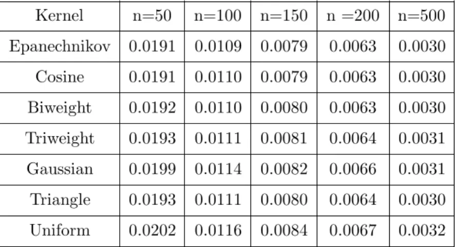
Kernel n=50 n=100 n=150 n =200 n=500 Epanechnikov 0.0191 0.0109 0.0079 0.0063 0.0030 Cosine 0.0191 0.0110 0.0079 0.0063 0.0030 Biweight 0.0192 0.0110 0.0080 0.0063 0.0030 Triweight 0.0193 0.0111 0.0081 0.0064 0.0031 Gaussian 0.0199 0.0114 0.0082 0.0066 0.0031 Triangle 0.0193 0.0111 0.0080 0.0064 0.0030 Uniform 0.0202 0.0116 0.0084 0.0067 0.0032

Table 2.2: Rate of Decrease of AMISE For All Seven Kernels as a Function of Sample Size

ranking is subject to several objections. First, how does the sample size affect each kernel’s performance? Second, how do these kernels rank if we need to estimate the cumulative density and reliability functions. Consistent with the objective of this chapter we will proceed to evaluate these kernels with a new bandwidth developed by Liu and Tsokos (2002), and with respect to small, medium and large sample size n.

(35)

2.4 New Ranking Based on Differences in Optimal Bandwidth for PDF, CDF, and Reliability Functions

In this section we turn our attention to the KDE of the cumulative distribution function F(x). The properties of the KDE of F(x) will help us study the KDE of the reliability function R(x), the failure function h(x) and the cumulative failure function H(x) defined in Chapter 1. The following theorem, derived in Liu and Tsokos (2002), will help us show that the optimal bandwidth for PDF is not optimal for CDF. This result will be important in Chapter 3 when we examine the reliability function of the Gumbel distribution and the concept of target time under desired reliability.

Theorem 2.4.1. Let F(x) be the cdf of f(x) and assume f(x) possesses the second

derivative. Then AMISE( ˆF(x)) = 1 4h 4_k2 2 Z +∞ −∞ f′2(x)dx+ 1 n Z +∞ −∞ F(x)(1₋F(x))dx

Proof. Integrating the expression for the bias of f(ˆx) given by (2.3.4) we obtain

bias( ˆF(x)) =EF(ˆx)₋F(x) = 1 2h

2_k

2f′(x). (2.4.1)

Also Nadaraya (1964) derived

V arFˆ(x) = 1

nF(x)(1−F(x)) +o( 1

n) (2.4.2)

Combining the two expressions above and integrating over the real line we get the expression for AMISE( ˆF(x))

Since the kernel density estimate of the reliability function is given by ˆ

(36)

we may make the following inference about the bias and variance of ˆR(x) : bias( ˆR(x)) =ER(ˆx)₋R(x) =₋1 2h 2_k 2f′(x). (2.4.3) and V arR(ˆx) = 1 nR(x)(1−R(x)) +o( 1 n) (2.4.4)

Recall that the optimal bandwidth estimate for PDF is given by hoptimal = [

C(K) k2

2C(f′′)

]15n−15

Since AMISE( ˆF(x)) can be written as AMISE( ˆF(x)) = 1 4h 4_k2 2 Z +∞ −∞ f′2(x)dx+ 1 n Z +∞ −∞ F(x)(1₋F(x))dx

upon closer study of the expression for AMISE( ˆF(x)) we may conclude the following:

(i) When h is chosen so that n14 → ∞, the bias part dominates, that is AMISE( ˆF(x)) = 1 4h 4_k2 2 Z +∞ −∞ f′2(x)dx and nAMISE( ˆF(x)) _{→ ∞}.

(ii) When the bandwidth h is small so that hn14 → 0 , the variance part dominates, thus AMISE( ˆF(x)) = 1 n Z +∞ −∞ F(x)(1₋F(x))dx Also, if we let h = an−14, AMISE( ˆF(x)) = 1 n Z +∞ −∞ F(x)(1₋F(x))dx+m n, m >0

(37)

so AMISE( ˆF(x)) attains its minimum value 1 n Z +∞ −∞ F(x)(1₋F(x))dx when h = o(n−1 4)

(iii) It was shown earlier that for the kernel density estimate f(ˆx)) , the optimal bandwidth is hoptimal = [ C(K) k2 2C(f′′) ]15n−15

It is obvious that hoptimal does not satisfy the condition hoptimaln

1

4 → 0 ,

so hoptimal is no longer optimal for the kernel cdf estimate ˆF(x) . The same

argument can be extended to conclude that hoptimal is no longer optimal for the

kernel estimate of the reliability function ˆR(x)

Visual Inspection Procedure to Determine Optimal Bandwidth for CDF and Reliability Functions

The following four step procedure was proposed by Liu and Tsokos (2002) as a visual inspection method to arrive at the optimal value of the bandwidth h for a given kernel estimate of cdf. This an important procedure that is relevant to the kernel density estimation of the cumulative distribution function F(x) and the reliability function R(x) We will test its effectiveness on the estimates of the cumulative distribution function and the reliability function for the Gumbel distribution presented in the next chapter.

(i) Choose a positive number h1 and an integer k.

(ii) For h = ih1

k , i = 1, 2, ... k calculate the corresponding ˆRn and display their

graphs.

(iii) If these k graphs look almost the same, choose a bigger h1 and go back to step

(38)

(iv) Find i∗ _{such that the graphs before} _i∗ _{look very similar and the graphs after}

i∗ _{look quite different from before.}

(v) Choose any h = ih1

k , i < i∗ and compute ˆRn.

The rationale for the above procedure lies in the fact that the change of AMISE( ˆFn)

follows a distinctive changing pattern of ˆFn as h increases from 0. When h is small

so that h = o(n−1

4) , the variance term in AMISE( ˆF_n) dominates and so

AMISE( ˆF(x)) = 1 n

Z +∞

−∞

F(x)(1₋F(x))dx

As h becomes larger such that hn14 → c6= 0 , both the squared-bias and the variance terms in AMISE( ˆFn) dominate equally, that is

AMISE( ˆF(x)) = 1 n Z +∞ −∞ F(x)(1₋F(x))dx+m n, m >0

As h increases even further so that hn14 → ∞, the bias term dominates and we have AMISE( ˆF(x)) = 1 4h 4_k2 2 Z +∞ −∞ f′2(x)dx

so that nAMISE( ˆF(x)) _{→ ∞} and the minimum is attained for h = o(n−14) . This means that when h varies from 0 toward the positive direction, AMISE( ˆFn) stays

almost the same at the value of O(n−1_{). So, during this stage the estimates ˆ}_F n will

look very similar. After h exceeds a certain value, AMISE( ˆFn) will increase rapidly

at a rate of O(h4_{) and the new estimates of ˆ}_F

n will deviate from the true F(x) quite

significantly. In terms of how the pilot bandwidth estimate should be chosen, the optimal bandwidth for PDF is a natural choice since it is always higher than the optimal bandwidth for cdf. The most intuitive choice for the pilot bandwidth under the assumption of normality, is

hpilot = 1.06min(ˆσ,

ˆ IQR

1.34)n

(39)

where ˆσ is the estimate of the sample standard deviation and IQRˆ is the interquartile range (Silverman 1986). In case of long tailed distribution and possible outliers, a robust estimate of ˆσ is more preferable and is usually taken to be

ˆ

σ = median(|xi−mˆ |) 0.6745

where ˆm denotes the sample median (Hogg 1979) In order to study how Silverman’s ranking of kernels may have changed under the new optimal bandwidth, we performed an extensive numerical study using the Gumbel probability distribution. The study was conducted in the following manner:

(i) We simulated m (m = 50, 100, 200) Gumbel distribution location parameters µ from the uniform distribution.

(ii) In order to see what effects the increase of variance has on our estimates, we let the scale parameter of the Gumbel distribution σ equal to 1, 2 and 4 respectively. (iii) Using the obtained m pairs of µ and σ, we generated n (n = 15, 30, 50, 100, 200) observations from the Gumbel PDF and obtained reliability estimates under Silverman’s and Liu’s optimal bandwidths and all seven kernels.

(iv) For comparison purposes, we calculated AMISE between the true reliability and the corresponding Silverman’s and Liu’s estimates, and ranked the kernels according to its size.

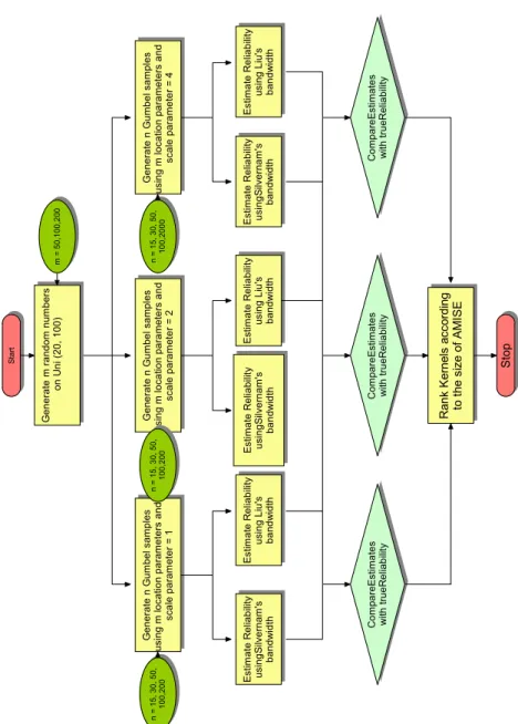
The schematic diagram of our numerical study is presented in figure 2.8. The results in tables 2.3-2.5 represent the average AMISE across all samples of size n and for varying values of σ for the average values of the pilot bandwidth hpilot, Silverman’s

bandwidth hopt, and Liu-Tsokos optimal bandwidth h∗ . Specifically, we calculated

the estimated AMISE across all samples n where

AMISE(Rn(t), R(t)) = N X i=1 Z (Rn(t)−R(t))2dt N ,

(40)

Figure 2.8: Numerical Study of Kernel Ranking

across all failure times t for the reliability function R(t), with N being the number of simulations. With respect to the evaluation of two selected optimal bandwidths, namely Silverman’s hopt and Liu-Tsokos’s h∗, as a function of the selected kernels,

(41)

er-ror. Using Liu-Tsokos bandwidth the effectiveness of all kernels was evaluated, with the top three kernels being the Epanechnikov, Cosine and Gaussian. Tables 2.3-2.5 suggest that for sample size n > 100 we obtain approximately the same probability density function subject to the same bandwidth. Since the Gaussian kernel offers several analytic advantages we conclude that Gaussian kernel should be used. Fur-thermore, the Gaussian kernel seems to be more stable as we increase the variance. For sample size n < 100 we have found that Epanechnikov kernel density function in conjuction with optimal bandwidth will give the best estimates. The increase in variance σ had no effect on the ranking of our kernels. Next we proceed to study

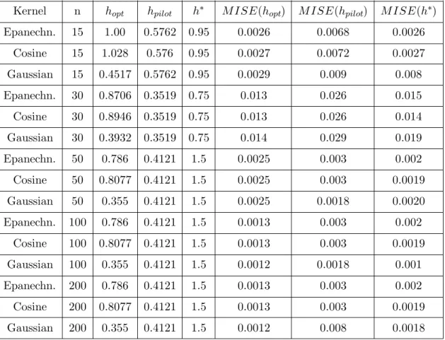
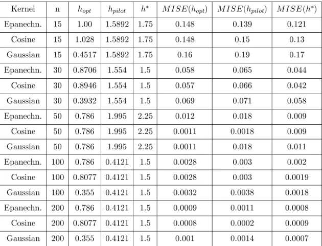
Kernel n hopt hpilot h∗ M ISE(hopt) M ISE(hpilot) M ISE(h∗)

Epanechn. 15 1.00 0.5762 0.95 0.0026 0.0068 0.0026 Cosine 15 1.028 0.576 0.95 0.0027 0.0072 0.0027 Gaussian 15 0.4517 0.5762 0.95 0.0029 0.009 0.008 Epanechn. 30 0.8706 0.3519 0.75 0.013 0.026 0.015 Cosine 30 0.8946 0.3519 0.75 0.013 0.026 0.014 Gaussian 30 0.3932 0.3519 0.75 0.014 0.029 0.019 Epanechn. 50 0.786 0.4121 1.5 0.0025 0.003 0.002 Cosine 50 0.8077 0.4121 1.5 0.0025 0.003 0.0019 Gaussian 50 0.355 0.4121 1.5 0.0025 0.0018 0.0020 Epanechn. 100 0.786 0.4121 1.5 0.0013 0.003 0.002 Cosine 100 0.8077 0.4121 1.5 0.0013 0.003 0.0019 Gaussian 100 0.355 0.4121 1.5 0.0012 0.0018 0.001 Epanechn. 200 0.786 0.4121 1.5 0.0013 0.003 0.002 Cosine 200 0.8077 0.4121 1.5 0.0013 0.003 0.0019 Gaussian 200 0.355 0.4121 1.5 0.0012 0.008 0.0018

Table 2.3: Mean Integrated Square Error (MISE) for the Top Three Bandwidths for Data

From Gumbel (n=15, 30, 50, 100, 200, σ= 1 )

(42)

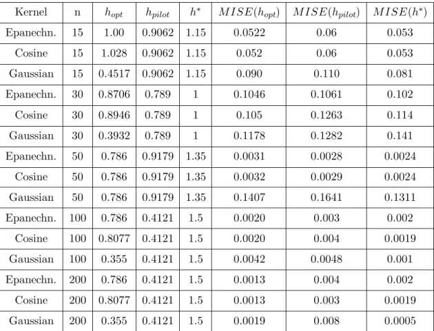
Kernel n hopt hpilot h∗ M ISE(hopt) M ISE(hpilot) M ISE(h∗) Epanechn. 15 1.00 0.9062 1.15 0.0522 0.06 0.053 Cosine 15 1.028 0.9062 1.15 0.052 0.06 0.053 Gaussian 15 0.4517 0.9062 1.15 0.090 0.110 0.081 Epanechn. 30 0.8706 0.789 1 0.1046 0.1061 0.102 Cosine 30 0.8946 0.789 1 0.105 0.1263 0.114 Gaussian 30 0.3932 0.789 1 0.1178 0.1282 0.141 Epanechn. 50 0.786 0.9179 1.35 0.0031 0.0028 0.0024 Cosine 50 0.786 0.9179 1.35 0.0032 0.0029 0.0024 Gaussian 50 0.786 0.9179 1.35 0.1407 0.1641 0.1311 Epanechn. 100 0.786 0.4121 1.5 0.0020 0.003 0.002 Cosine 100 0.8077 0.4121 1.5 0.0020 0.004 0.0019 Gaussian 100 0.355 0.4121 1.5 0.0042 0.0048 0.001 Epanechn. 200 0.786 0.4121 1.5 0.0013 0.004 0.002 Cosine 200 0.8077 0.4121 1.5 0.0013 0.003 0.0019 Gaussian 200 0.355 0.4121 1.5 0.0019 0.008 0.0005

From Gumbel (n=15, 30, 50, 100, 200, σ= 2 )

2.5 Bandwidth Robustness

Now we wish to take a look at how AMISE changes as we incrementally decrease and increase hoptimal under Liu’s five-step procedure for each kernel, that is wish to

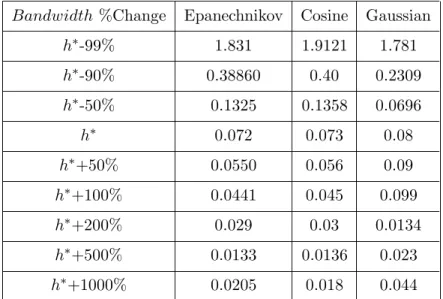
study how robust the optimal bandwidth for each kernel is by observing the rate of change of AMISE as the optimal bandwidth for each kernel uniformly decreases or increases. In order to do this we have used the same numerical procedure represented by figure 2.8 except that we studied how sensitive the change in bandwidth selection is with respect to change in AMISE for a fixed bandwidth for each of the three kernels. To study the rate of increase of AMISE we have used the ratio of two consecutive

(43)

Kernel n hopt hpilot h∗ M ISE(hopt) M ISE(hpilot) M ISE(h∗) Epanechn. 15 1.00 1.5892 1.75 0.148 0.139 0.121 Cosine 15 1.028 1.5892 1.75 0.148 0.15 0.13 Gaussian 15 0.4517 1.5892 1.75 0.16 0.19 0.17 Epanechn. 30 0.8706 1.554 1.5 0.058 0.065 0.044 Cosine 30 0.8946 1.554 1.5 0.057 0.066 0.042 Gaussian 30 0.3932 1.554 1.5 0.069 0.071 0.058 Epanechn. 50 0.786 1.995 2.25 0.012 0.018 0.009 Cosine 50 0.786 1.995 2.25 0.0011 0.0018 0.009 Gaussian 50 0.786 1.995 2.25 0.0011 0.018 0.011 Epanechn. 100 0.786 0.4121 1.5 0.0028 0.003 0.002 Cosine 100 0.8077 0.4121 1.5 0.0028 0.003 0.0019 Gaussian 100 0.355 0.4121 1.5 0.0032 0.0038 0.0018 Epanechn. 200 0.786 0.4121 1.5 0.0009 0.0011 0.0008 Cosine 200 0.8077 0.4121 1.5 0.0008 0.0002 0.0009 Gaussian 200 0.355 0.4121 1.5 0.001 0.0014 0.0007

From Gumbel (n=15, 30, 50, 100, 200, σ= 4 ) AMISE’s defined as AMISErate= AMISEi AMISEi−1 , i= 1, ..., l (2.5.1) where the subscript indicates an i-percent of the bandwidth increase or decrease in bandwidth. The results are presented in Tables 2.6-2.8.We fixed the top three kernels, namely Epanechnikov, Cosine and Gaussian, and studied the behavior of AMISE under the same numerical study as given by figure 2.6. The optimal bandwidth h∗

was varied in both directions by a certain percentage and sample size n= 20, 50, and 100. The results are given in tables 2.6-2.8 and indicate that the smallest increases in AMISE were present under the Gaussian Kernel as we fixed the kernel and increased

(44)

the sample size. This suggests that the Gaussian kernel is more stable as we increase the sample size. Under the optimal bandwidth for each kernel we have found that the

Bandwidth %Change Epanechnikov Cosine Gaussian

h∗-99% 1.831 1.9121 1.781 h∗-90% 0.38860 0.40 0.2309 h∗-50% 0.1325 0.1358 0.0696 h∗ 0.072 0.073 0.08 h∗+50% 0.0550 0.056 0.09 h∗+100% 0.0441 0.045 0.099 h∗+200% 0.029 0.03 0.0134 h∗+500% 0.0133 0.0136 0.023 h∗+1000% 0.0205 0.018 0.044

Table 2.6: AMISE Rate of Change for h∗, n = 20

h∗-99% 2.328 2.786 0.9097 h∗-90% 0.1415 0.1656 0.0652 h∗-50% 0.025 0.0305 0.009 h∗ 0.0097 0.012 0.004 h∗+ 50% 0.0058 0.007 0.0039 h∗+ 100% 0.0043 0.0496 0.0052 h∗+ 200% 0.0037 0.0037 0.0098 h∗+ 500% 0.0088 0.0066 0.0277 h∗+ 1000% 0.0252 0.0195 0.049

Table 2.7: AMISE Rate of Change for h∗, n = 50

rate of increase in AMISE for the top three kernels is virtually identical, which leads to conclude that an increase in h∗ _{for a given kernel will produce roughly the same}

(45)

is robust with respect to the choice of kernel. As expected as n increases, AMISE decreases. We also notice that AMISE is higher if we choose a much lower value for h∗ _{rather than a higher value, so the penalty of overestimating the bandwidth is}

lower than the penalty for underestimating. Also, AMISE does not increase much as we increase the bandwidth. From table 2.5 we see that if we increase h∗ _{ten fold,}

AMISE is ”only” 0.0415 for Epanecnikov, 0.0399 for Cosine and 0.048 for the Gaussian kernel. We know that if the bandwidth increases we run the risk of oversmoothing which may hide important features of the data, such as bimodality, and cause us to draw wrong conclusions. It should be noted that our simulation has indicated that

lim

i→∞AMISErate= 1 .

h∗-99% 0.5234 0.5411 0.381 h∗-90% 0.0404 0.042 0.031 h∗- 50% 0.0073 0.0076 0.0042 h∗ 0.0021 0.0022 0.0022 h∗+ 50% 0.0023 0.0023 0.0031 h∗+ 100% 0.0029 0.0029 0.0047 h∗+ 200% 0.0056 0.0053 0.0095 h∗+ 500% 0.0198 0.0187 0.027 h∗+ 1000% 0.0415 0.0399 0.048

(46)

2.6 Conclusion

In this chapter we studied all seven symmetric kernels used in kernel density esti-mation and applied the asymptotic mean square error to rank the top three kernels different from Silverman (1986). Our ranking places the Gaussian kernel third, after Epanechnikov and Cosine kernels. This was done under a simple visual procedure introduced by Liu and Tsokos (2002), which produces an optimal cdf and reliability kernel density estimates and is to be used in the rest of our study. We showed that sample size n is important in selecting the appropriate kernel function. Generally, the Epanechnikov kernel performs better for sample size n < 100, while all three are roughly the same for n _≥ 100. Since the Gaussian kernel offers analytic and numeric simplicity, we recommend the Gaussian kernel be used for n _≥ 100. We also showed that hoptimal for the top three kernels is robust with respect to the choice of

the kernel, as well as the sample size n. The findings in our present chapter will be utilized in reliability and the modeling of floods.

(47)

3 Ordinary, Bayes, Empirical Bayes, and Kernel Density Reliability Estimates for the Gumbel Failure Model

3.1 Introduction

Extreme value probability distributions have been used effectively to model various problems in engineering, environment, business, etc. Some key references are Burton and Markopoulos (1985), Naess (1998), Osella et. al. (1992), Ramachandran (1982) Rao et al. (1997), Sastry and Pi (1991), Silbergleit (1996), Suzuki and Ozaha (1994), Tsokos (1999), and Yue (2000). A recent book by Kotz and Nadarajah (2000) lists over fifty applications, ranging from accelerated life testing to earthquakes, floods, horse racing, rainfall, queues in supermarkets, sea currents, wind speeds, and race track records. Tsokos (1999) analyzed a modified extreme value distribution and derived the minimum variance unbiased (MVU) and Bayesian estimates of the reli-ability function under the general uniform, exponential, and inverted gamma priors, and the mean square error loss function. Using his work as a foundation, the objective of this study is to modify the classical Gumbel, or double exponential, probability distribution to characterize the failure times of a given system. The modification is necessary in order to obtain analytically tractable estimates of the desired functions and to ensure that time to failure can be considered modified to reliability analysis. We are interested in obtaining ordinary and Bayesian estimates of the Gumbel reli-ability, failure rate, and cumulative failure rate functions. In addition to obtaining maximum likelihood (ML) and MVU estimates, we have developed the subject model in Bayes and empirical Bayes settings. We are also interested in obtaining ordinary, Bayes, and empirical Bayes estimates of the target time tc subject to a desired and

(48)

specified reliability. That is, we want to know what the time to failure tc is with

at least (1 - c)100% assurance. For example, we want to be at least 95% certain that the system will be operable to time t0.05. In the Bayesian setting, we use the

natural conjugate prior under the mean square error loss function. Lindley’s approx-imation procedure is used to obtain numerical results that illustrate the usefulness of the study. Finally, we assume the failure data does not fit the Gumbel probability distribution, and consistent with our results in chapter 2, obtain the kernel density estimates for the Gumbel reliability. In addition to analytical results, we have con-ducted an extensive numerical simulation in order to illustrate the usefulness of the inference procedures discussed. In summary, after introducing the modified Gumbel failure model in section 3.2, we aim to accomplish the following:

(i) In section 3.3, present the ML and MVU estimates of reliability, failure rate, cumulative failure rate functions, and the target time subject to a specified reliability tc.

(ii) In section 3.4, derive the Bayesian and empirical Bayes estimates of reliability, failure rate, cumulative failure rate functions, and the target time tc, under the

natural conjugate prior and a square error loss function.

(iii) In section 3.5, present the non-parametric kernel density estimates of the func-tions under study.

(iv) In section 3.6, perform an extensive numerical analysis to compare the estimates and illustrate the usefulness of the methodology. In this section, we will use the five step procedure introduced in chapter 2 to obtain the optimal kernel density estimates of reliability, failure rate, cumulative failure rate, and target time tc

to ascertain how well the kernel density estimates perform when compared with their parametric counterparts in both ordinary and Bayesian settings.

(49)

3.2 The Gumbel Failure Model

For the Gumbel failure model, the probability distribution function (PDF) and the cumulative distribution function (CDF) of the failure time at time t are given, re-spectively, by f(t;µ, σ) = 1 σe −t−µ σ −e− t−µ σ ,_−∞< t, µ <_∞, σ >0 (3.2.1) and F(t;µ, σ) =P r(X _≤t) =e−e−t−_σµ , (3.2.2)

where µ and σ are the location and scale parameters. The likelihood function L(µ, σ), is given by L(t;µ, σ) =σ−nexp_{− n X i=1 ti−µ σ − n X i=1 exp(₋ti−µ σ )}. (3.2.3) The Gumbel failure model has been used in fire protection, insurance problems, pre-diction of earthquake magnitudes, carbon dioxide levels in the atmosphere, and high return levels of wind speeds in the design of structures among others. Based on record values, Ahsanullah (1990, 1991) obtained the maximum likelihood (ML), best linear invariant (BLI) and minimum variance unbiased (MVU) estimators of the Gumbel location and scale parameters, and Ali Mousa et al. (2001) obtained the Bayesian estimators of the same under Jeffrey’s non-informative prior. In the present study, we shall modify the subject model and apply it in reliability in ordinary, Bayesian and empirical Bayes settings. In the next section, we consider the ordinary estima-tors, namely the maximum likelihood (ML) and minimum variance unbiased (MVU) estimators. To our knowledge, the MVU estimators have not been derived, so the derivation is presented.

(50)

3.3 Reliability Modeling

Let t1, t2, ... , tn be the failure times that follow the Gumbel PDF given by (3.2.1).

The reliability at time t of a system whose life follows the probability law f(x; θ) is given by

R(t;θ) = Z ∞

t

f(x;θ)dx= 1₋F(t) (3.3.1) Under the same reliability function R(t;θ) , the failure rate and cumulative failure rate functions are given by

h(t) = − ∂R(t;θ) ∂t R(t;θ) (3.3.2) and H(t) =₋ln(R(t;θ)). (3.3.3) The failure rate function can be interpreted as the probability, per unit of time, that the item will fail after time t, given that the item has operated up to time t. In other words, the failure rate function can be interpreted as the probability of instantaneous failure, given that the item has operated up to time t.

If we let

g(t;σ) =e−e−_σt

and

θ =eµσ,

then the CDF and reliability functions of the classical Gumbel failure model can be written as

F(t;θ) = [g(t)]θ (3.3.4) and

R(t;θ) = 1₋[g(t)]θ. (3.3.5) Note that g(t) is monotone increasing and R(t;θ) is bounded from above and below. In addition to parameter the scale σ > 0, the new parameter θ is also positive.

(51)

Since failure times are positive quantities, this will allow for better consistency of pa-rameters. Using the new parameterization, the probability density and the likelihood functions can be written as

f(t;θ) = ∂F(t;θ) ∂θ = [g(t)] (θ−1)_[_g₍_t_)] ′ (3.3.6) and L(t;θ) =θn_Π_g_′₍_t i)[g(ti)]θ−1. (3.3.7)

The failure rate and cumulative failure rate functions are respectively given by h(t, θ) = θg′(t)[g(t)]

θ

g(t)(1₋g(t)θ₎ (3.3.8)

and

H(t, θ) = ₋ln(1₋[g(t)]θ). (3.3.9) By taking the natural logarithm of both sides of equation (3.3.4) and solving for t, we obtain the expression for the target time tc under the desired reliability (1 - c)100%

given by

tc = (ln(−

θ ln(c)))

σ_. _(3.3.10)

The maximum likelihood estimates (MLE) for σ and θ can be derived from equations (3.2.3) and (3.3.7) by solving ∂lnL

∂σ = 0 and ∂lnL

∂θ = 0, from which we obtain the ML

estimates ˆ σM L+ Σtie−ti/ˆσ Σe−ti/ˆσ = ¯t (3.3.11) and ˆ θM L= n G, (3.3.12) where G=₋ n X i=1 lng(ti). (3.3.13)

(52)

Equations (3.3.11) and (3.3.12) are not analytically tractable and must be solved numerically to obtain approximate MLE’s of σ and θ. By the invariance property of the MLE’s, we can obtain the ML estimates of the subject functions by replacing parameters σ and θ with their ML estimates ˆσ and ˆθ.

In complex systems, the cumulative effect of bias might be quite considerable and a system might prove unsatisfactory during operation time. For this reason, we derive the minimum variance unbiased (MVU) estimators of the functions for the modified Gumbel failure model and apply them to reliability analysis. In order to derive the MVU estimators, we need to find a sufficient and complete statistic for θ and find its distribution. Given a sample of size n of failure times, t1, t2, ... , tn, and the

cumulative distribution function in (3.3.4) by the Neymann factorization theorem and using the likelihood function given by (3.3.7), it is easily shown that the quantity G = -Pn

i=1lng(ti) is sufficient and complete for θ. To find the distribution of G, we use

the characteristic function argument. If we let p(t) = -ln(g(t)), then the characteristic function of p(t) is φ(w) = E(eitp(t)) = Z ∞ 0 ewp(t)θg′(t)g(t)θ−1ds or φ(w) = Z ∞ 0 ewsθe−θsds= θ θ₋w,

which is the characteristic function for the exponential random variable. Using the property that the Gamma probability distribution represents the sum of n exponen-tially distributed random variables, we conclude that G is distributed as a Gamma random variable with parameters α = n and β = θ. Its probability density function is given by f(G;n, θ) = G n−1 Γ(n)θ n_e−θG_, −lng(t)< G < _∞. (3.3.14) By the Rao-Blackwell and Lehman-Scheffe theorems, we conclude that the MVU

(53)

estimate of the reliability function R(t) is given by ˆ RM V U(t) = 1−(1 + lng(t) G ) n−1_, −lng(t)< G < _∞. (3.3.15) This result follows by noting that G is a complete sufficient statistic, and that the expected value of the MVU reliability estimate equals the true reliability estimate, that is ERˆM V U(t) = 1− Z ∞ −lng(t) (1 + lng(t) G ) n−1Gn−1 Γ(n)θ n_e−θG_dG ERˆM V U(t) = 1− Z ∞ 0 un−1 Γ(n)θ n_eθ(u−lng(t))_du_{= 1} −g(t)θ, so that ERˆM V U(t) =R(t)

Likewise, the MVU estimators for the failure rate and cumulative failure rate func-tions, and target time subject to a specified reliability are given by:

ˆ hM V U(t) = ∂RˆM V U(t) ∂t ˆ RM V U(t) (3.3.16) ˆ HM V U(t) = −ln( ˆRM V U(t)) (3.3.17) and ˆ tM V U(α) =−σln(G−Gα 1 n−1). (3.3.18)

In the following section, we proceed to derive the Bayesian estimates for the modified Gumbel failure model.

3.4 Bayes Estimators of Reliability

In this section, we consider a Bayesian analysis of reliability for the modified Gumbel failure model under the influence of square error loss and the natural conjugate prior. We also derive the empirical Bayes estimates for the modified Gumbel failure model.

(54)

Recall that given a sample of size n of failure times, t1, t2, ... , tn, the modified

Gumbel reliability function is given by

R(t;θ) = 1₋[g(t)]θ where

g(t;σ) =e−e−σt

and

θ(µ, σ) =eσµ.

We assume that the parameter σ is fixed and that the parameter θ behaves as a random variable. This implies that the location parameter µ of the classical Gumbel probability distribution behaves as a random variable. In the previous section, we showed that statistic

G=₋

n

X

i=1

lng(ti)

is sufficient and complete for θ and is distributed as a Gamma random variable. Therefore, we are justified in assuming that the natural conjugate prior of parameter θ follows the Gamma probability distribution with parameters α and β, so that the natural conjugate prior has the form

g(θ;α, β) = β

α

Γ(α)θ

α−1_e−βθ_.

The joint PDF of t1,...,tn is given by

L(t;θ) = Z f(t_|θ)g(θ;α, β)dθ L(t;θ) = Z ∞ 0 βα Γ(α)θ n+α−1_e−βθ_Π_g ′(ti)[g(ti)]θ−1dθ, which gives L(t;θ) = β α_Γ(_n₊_α₎ Γ(α)(β+G)n+αΠ g_′(t) g(t). (3.4.1)