Overconfidence of Professionals and Lay Men: Individual Differences Within and Between Tasks?

S

ONDER

F

ORSCHUNGS

B

EREICH

504

Rationalit ¨atskonzepte,

Entscheidungsverhalten und

¨okonomische Modellierung

Overconfidence of Professionals and Lay Men: Individual Differences Within and Between Tasks?

Markus Glaser∗

and Thomas Langer∗∗

and Martin Weber∗∗∗

April 2005

Financial support from the Deutsche Forschungsgemeinschaft, SFB 504, at the University of Mannheim, is gratefully acknowledged.

∗_{Sonderforschungsbereich 504, email: [email protected]}

∗∗_{Westf ¨alischen Wilhelms-Universit ¨at M ¨unster Lehrstuhl f ¨ur BWL, insbesondere Finanzierung, email:} [email protected]

∗∗∗_{Lehrstuhl f ¨ur ABWL, Finanzwirtschaft, insb. Bankbetriebslehre, email:} [email protected]

Overconfidence of Professionals and Lay Men:

Individual Differences Within and Between Tasks?

Markus Glaser, Thomas Langer, and Martin Weber∗

April 26, 2005

Abstract

Overconfidence can manifest itself in various forms. For example, people think that their knowledge is more precise than it really is (miscalibration) and they believe that their abilities are above average (better than average effect). The questions whether judgment biases are related or whether stable individual differences in the degree of overconfidence exist, have long been unexplored. In this paper, we present two studies that analyze whether professional traders or investment bankers who work for international banks are prone to judgment biases to the same degree as a population of lay men. We examine whether there are robust individual differences in the degree of overconfidence within various tasks. Furthermore, we analyze whether the degree of judgment biases is correlated across tasks. Based on the answers of 123 professionals, we find that expert judgment is biased. In most tasks, their degrees of overconfidence are significantly higher than the respective scores of a student control group. In line with the literature, we find stable individual differences within tasks (e.g. in the degree of miscalibration). However, we find that correlations across distinct tasks are sometimes insignificant or even negative. We conclude that some manifestations of overconfidence, that are often argued to be related, are actually unrelated.

Keywords: Overconfidence, Judgment Biases, Individual Differences, Expert Judgment

JEL Classification Code: C9, G1

∗_{Markus Glaser is from the Lehrstuhl f¨ur Bankbetriebslehre, Universit¨at Mannheim, L 5, 2, 68131 Mannheim. E-Mail:}

[email protected]. Thomas Langer is from the Lehrstuhl f¨ur Finanzierung, Universit¨at M¨unster, Univer-sit¨atsstraße 14-16, 48143 M¨unster. E-Mail: [email protected]. Martin Weber is from the Lehrstuhl f¨ur Bankbetriebslehre, Universit¨at Mannheim, L 5, 2, 68131 Mannheim and CEPR, London. E-Mail: [email protected]. We would like to thank Andreas Trauten and seminar participants at the University of Mannheim, the 9th Behavorial Decision Research in Management (bdrm) Conference, Duke University, Durham, and the Society for Judgment and Decision Making (SJDM) Annual Conference, Minneapolis, for valuable comments and insights. Financial Support from the Deutsche Forschungsgemeinschaft (DFG) is gratefully acknowledged.

Overconfidence of Professionals and Lay Men:

Individual Differences Within and Between Tasks?

Abstract

Overconfidence can manifest itself in various forms. For example, people think that their knowledge is more precise than it really is (miscalibration) and they believe that their abilities are above average (better than average effect). The questions whether judgment biases are related or whether stable individual differences in the degree of overconfidence exist, have long been unexplored. In this paper, we present two studies that analyze whether professional traders or investment bankers who work for international banks are prone to judgment biases to the same degree as a population of lay men. We examine whether there are robust individual differences in the degree of overconfidence within various tasks. Furthermore, we analyze whether the degree of judgment biases is correlated across tasks. Based on the answers of 123 professionals, we find that expert judgment is biased. In most tasks, their degrees of overconfidence are significantly higher than the respective scores of a student control group. In line with the literature, we find stable individual differences within tasks (e.g. in the degree of miscalibration). However, we find that correlations across distinct tasks are sometimes insignificant or even negative. We conclude that some manifestations of overconfidence, that are often argued to be related, are actually unrelated.

Keywords: Overconfidence, Judgment Biases, Individual Differences, Expert Judgment

1

Introduction

Overconfidence can manifest itself in various forms. People think that their knowledge is more precise than it really is (miscalibration, see Lichtenstein, Fischhoff, and Phillips (1982)), they believe that their abilities are above average (better than average effect, see Svenson (1981) and Taylor and Brown (1988)), they think that they can control random tasks, and they are excessively optimistic about the future (illusion of control and unrealistic optimism, see Langer (1975), Presson and Benassi (1996), and Weinstein (1980)). The questions whether these judgment biases or degrees of overconfidence are related or whether there are robust individual differences in the degree of overconfidence have long been unexplored. Recently, psychological research has started to investigate whether there are stable individual differences in reasoning or decision making competence (see, for example, Parker and Fischhoff (2001), Stanovich and West (1998), and Stanovich and West (2000)). However, experimental studies almost exclusively focus on judgments biases of a student population. In a finance context, it is often argued that not much can be learned from these experiments about real-world financial markets because professional investors have a much higher influence or price impact than individual investors and are thus more important in the process of determining market allocations and market

outcomes.1

In our paper, we present two experimental studies that contribute to the above mentioned issues by pursuing the following main goals. We analyze whether financial market pro-fessionals (traders, investment bankers) who work for a large German bank and a large international bank are subject to judgment biases to the same degree as a population

of students. We examine whether there are stable individual differences in the degree of overconfidence within various specific task. Furthermore, we analyze whether the degree of judgment biases is correlated across tasks, i.e. whether the same individuals are more biased in their judgments than others in a variety of domains.

In one study, professional traders and a student control group participated in a multi-phase experiment that was in part conducted via the internet. This experiment consisted of various distinct tasks. Subjects were asked to state subjective confidence intervals for several knowledge questions to measure their degree of miscalibration. They had to give volatility estimates for various stocks and stock indices over different forecast horizons. Moreover, they predicted the development of artificially generated time-series charts by stating confidence intervals. Finally, subjects gave self-assessments about their own per-formance and their perper-formance relative to other experimental subjects.

In the next study, investment bankers and a student control group participated in a questionnaire study that replicates some parts of the first study (subjective confidence interval questions, self-assessments about their own performance and their performance relative to other experimental subjects).

Using the data of these two studies, we address the following questions:

• Are individuals biased?

• Does expertise mitigate or exacerbate biases, i.e. are professionals better or worse

than students?

• Are there robust individual differences within the tasks considered, i.e. are some

• Are there individual differences across tasks, i.e. are subjects who are more biased in one task also more biased in another task?

Answers to these questions are important for theory building in economics and finance. In finance, for example, overconfidence is usually modeled as overestimation of the precision

of information.2 _{As a consequence, overconfident investors state confidence intervals for}

the future value of a risky asset that are too tight compared to the rational benchmark. Overconfidence models typically derive hypotheses like “expected trading volume of an in-vestor increases as overconfidence increases” (see, for example, Odean (1998), proposition 1). Some papers even refer to investors’ different degrees of overconfidence as different investor “types” (e.g. Benos (1998), p. 360). These overconfidence models thus implic-itly assume that there are stable individual differences in the degree of overconfidence within tasks. It is important to verify whether this is a sensible assumption for the tasks considered in such models.

Closely related is the question of whether the various facets of overconfidence mentioned at the beginning of the introduction are related, i.e. whether the overconfidence scores across tasks are positively correlated. Griffin and Brenner (2004), for example, argue that various facets of overconfidence might be linked. They present several theoretical perspectives on (mis)calibration, among them the most influential perspective, optimistic overconfidence. According to the authors, the optimistic overconfidence perspective builds, for example, on the better than average effect, unrealistic optimism, and illusion of control. By correlating overconfidence scores, we can test this theoretical perspective.

Our main results can be summarized as follows. Judgments of professionals are biased. In 2_{See Glaser, N¨oth, and Weber (2004) for a discussion of the overconfidence literature in finance.}

all tasks and in both studies, their degrees of overconfidence are higher than the respec-tive scores of the student control group. In most tasks, this difference is significant. In line with extant literature, we find stable individual differences within tasks (e.g. in the degree of miscalibration, as measured by confidence interval questions). However, we find that correlations across distinct tasks are sometimes insignificant or even negative. We conclude that some manifestations of overconfidence, that are often argued to be related, are actually unrelated.

The rest of this paper is organized as follows. The next section describes the general design of the two studies. Section 3 presents the tasks in more details and shows the results of the respective task. Section 4 presents the correlation across tasks and the differences between professionals and students. The last section discusses the results and concludes.

2

The Two Studies: Design and Experimental Subjects

2.1 Study 1

Study 1 consists of an experiment and a questionnaire part with four phases.3 _{In the first}

phase, a questionnaire was presented that asked for confidence intervals with respect to knowledge questions. In this phase, we also collected demographic data. The three other phases of the project were internet based. In pre-specified time windows subjects had to access a web page and log in to the experimental software. Each phase took about 30 minutes to complete. Overall, 33 professionals of a large German bank (i.e. all traders who work in the trading room of this bank) participated in the project. 29 of them 3_{In addition, there was a pre-experimental meeting in which we interviewed the professional subjects to better understand}

completed all parts of the study, the remaining subjects dropped out or missed a phase due to vacation or other reasons. Based on a self report in the first phase, 11 professionals assigned their job to the area “Derivatives”, 10 to the area “Proprietary Trading”, 12 to

the area “Market Making” and 6 to “Other Area”.4 _{The age of the professionals ranged}

from 23 to 55 with a median age of 33 years. 14 subjects had a university diploma and the median subject worked five years for the bank (range 0.5 to 37 years). In addition to the professionals, we had a control group of 75 advanced students, all specializing in Banking and Finance at the University of Mannheim. 62 of them completed all tasks. Their median age was 24 and ranged from 22 to 30. The control group was faced with exactly the same procedure as the professionals with the one exception that for administrative reasons the

questionnaire of phase 1 was filled out at the end not the beginning of the project.5

The study consists of the following parts or tasks that we will discuss comprehensively in

the next section:6

• Confidence intervals for 20 knowledge questions (ten questions concerning general

knowledge and ten questions concerning economics and finance knowledge).

• Self-assessment and assessment of own performance compared to others in knowledge

questions.

• 15 stock market forecasts via confidence intervals.

• Trend forecasting via confidence intervals.

4_{Subjects could assign themselves to more than one area.}

5_{We did not ask for gender in the questionnaire part as there were no female traders in the practitioner sample.}

6_{The study also consisted of other components (addressing, for example, the hindsight bias and the role of feedback)}

2.2 Study 2

In Study 1, we only have a low number of professionals participating. This is the reason why we try replicate and validate our results of Study 1 with a different sample and a larger number of professionals. Study 2 is therefore similar to the questionnaire part

of Study 1.7 _{90 investment bankers of an international bank and a control group of 76}

students participate in Study 2. 41 investment bankers worked in Frankfurt, 49 invest-ment bankers worked in London. The average age of an investinvest-ment banker is 34 (median 33). The London based investment bankers were slightly older than the Frankfurt based bankers (35.6 versus 32.4, on average). The age range in both cities was 23 to 50 years. In Frankfurt, there were 4 female and 37 male bankers. In London there were 12 female and 37 male investment bankers. The students, all specializing in Banking and Finance at the University of Mannheim again, were 24.3 years old on average (median 24). 17 students were female, 59 were male.

Study 2 consists of the following parts or tasks that are similar to the respective parts of

Study 1:8

• Confidence intervals for 20 questions (ten questions concerning general knowledge

and ten questions concerning economics and finance).9

• Self-assessment and assessment of own performance compared to others in knowledge

questions.

7_{However, it was not possible to replicate the internet based part of Study 1 with the subject pool of Study 2.}

8_{Additionally, there was another questionnaire part that was designed to measure the degree of the hindsight bias of}

subjects. These results will be presented in another paper.

9_{The only difference is that the economics and finance questions in Study 2 consist of 5 knowledge questions and 5 stock}

3

Results: Individual Differences Within Tasks?

3.1 Knowledge Questions: Confidence Intervals

The experimental subjects in both studies were asked to state upper and lower bounds of 90 % confidence intervals for ten questions concerning general knowledge and ten eco-nomics and finance questions. These questions can be used to measure the degree of

miscalibration.10

The questions were as follows:

For the following questions, please give two estimates each. The true answer to the questions (e.g. in the first question the age of pope Pius II at his death) should...

Lower Bound: ...with a high probability (95 %) not fall short of the lower bound.

Upper Bound: ... with a high probability (95 %) not exceed the upper bound.

We calculate two overconfidence scores: the number of correct answers that fall outside the 90 % confidence interval for general knowledge questions and economics and finance knowledge questions, respectively. For a well-calibrated subject the number of correct answers that fall outside the 90 % confidence interval should be about one out of ten.

10_{See, for example, Klayman, Soll, Gonz´ales-Vallejo, and Barlas (1999), Biais, Hilton, Mazurier, and Pouget (2005), Russo}

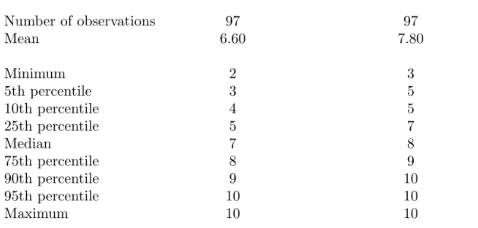
Table 1 presents the mean, minimum, maximum, and several percentiles of our first over-confidence score which is the number of correct answers that fall outside the 90 % confi-dence interval for general knowledge as well as economics and finance knowledge questions for Study 1 (the respective results of Study 2 are similar). The first observation is that

all subjects are overconfident. The minimum of the numbers of correct answers that fall

outside the 90 % confidence interval are 2 and 3, respectively. The median number of correct answers outside the stated intervals is 7 for general knowledge questions and 8 for economics and finance knowledge questions. The respective results of Study 2 are 7

and 5. Based on these values we define an overconfidence score (OC_knowledge) that is the

average of the two overconfidence scores based on general knowledge as well as economics and finance knowledge confidence interval questions presented above. We will use this score later in the paper.

The findings presented above are in line with prior research. Russo and Schoemaker (1992), for example, find a percentage of surprises (i.e. the percentage of the number of correct answers outside the stated intervals) in the range from 42 % to 64 %. Other studies find

percentages of surprises that are even closer to ours.11 _{Furthermore, Table 1 indicates}

large individual differences across subjects: The number of correct answers outside the stated intervals range from 2 to 10. In the remainder of this subsection, we explore this issue in greater detail.

The correlation of the two overconfidence scores in Study 1 is significantly positive. The

correlation coefficient is 0.6313 with ap-value less than 0.0001. The Spearman rank

corre-lation coefficient is 0.6589 (p-value<0.0001). In Study 2, the correlation is 0.3985 (p-value

11_{See, for example, Klayman, Soll, Gonz´ales-Vallejo, and Barlas (1999), Biais, Hilton, Mazurier, and Pouget (2005), Soll}

<0.0001). These results indicate stable individual differences in the degree of miscalibra-tion. To check the robustness of this result, we randomly split the ten general knowledge questions and the ten economics and finance knowledge questions into two groups of five

questions each.12 _{The four overconfidence scores are again calculated as the number of}

correct answers that fall outside the 90 % confidence interval. All six pairwise correlation

coefficients are significantly positive in Study 1. The highest p-value is 0.0136. The

cor-relation coefficients display values between 0.2498 and 0.4830 with an average of 0.4071. The Cronbach alpha is 0.7330. This value is higher than 0.7, which is often regarded as an acceptable reliability coefficient (see Nunnally (1978)). Biais, Hilton, Mazurier, and Pouget (2005) present a Cronbach alpha of 0.58 for similar questions in their paper. They argue that “the different items we use to measure miscalibration tend to be positively

correlated, although the correlation is only moderately strong”.13

In Study 2, we also find that all six pairwise correlation coefficients are significantly

positive with values between 0.1889 and 0.3317 (highestp-value is 0.0148). The Cronbach

alpha is 0.5931. Note that this value is lower than the alpha in Study 1 but higher than the alpha in the Biais, Hilton, Mazurier, and Pouget (2005) study. Thus, even five confidence interval questions are enough to reliably rank subjects with regard to their degree of miscalibration. These results strengthen our previous conjecture that there are stable individual differences in the degree of miscalibration. Our findings are in line with

prior research14 _{Klayman, Soll, Gonz´ales-Vallejo, and Barlas (1999), for example, also}

use the split-sample approach and find high correlations that are similar to ours in the 12_{See Klayman, Soll, Gonz´ales-Vallejo, and Barlas (1999), p. 225, for details on the split-sample approach.}

13_{See Biais, Hilton, Mazurier, and Pouget (2005), p. 297.}

14_{See Alba and Hutchinson (2000), Klayman, Soll, Gonz´ales-Vallejo, and Barlas (1999), Pallier, Wilkinson, Danthiir,}

degree of overconfidence across several sets or subsamples of confidence interval knowledge

questions.15

Gigerenzer (1991) argues that it is easy to make the overconfidence bias disappear. He confronted people with knowledge questions and asked them to pick one of two possible answers. Afterwards, subjects were asked to state a subjective probability estimate that their answer was correct. Such a design produces overconfidence in the respect that in each

set of questions that got assigned the same probabilityp to be correct, the proportion of

correct answers is in fact much lower than p. However, if subjects were asked in addition:

“How many of these questions do you think you got right?”16_{, the overconfidence bias}

disappeared as these estimates were close to the true relative frequencies. This study motivated the following two questions of our questionnaire:

• At the beginning of this questionnaire, we asked you to provide upper and lower

bounds for the answers to 10 general knowledge questions. For how many of these questions do you think the true answer is outside the range you gave?

(please give a number between 0 and 10)

• At the beginning of this questionnaire, we also asked you to provide upper and lower

bounds for the answers to 10 questions related to finance and economics. For how many of these questions do you think the true answer is outside the range you gave? (please give a number between 0 and 10)

In Study 1, the mean answers of these two questions are 4.18 and 4.64 respectively (the 15_{Klayman, Soll, Gonz´ales-Vallejo, and Barlas (1999), p. 240.}

medians are 4). In Study 2, we find similar values (3.63 and 3,89 with medians 3 and 4).These figures are indeed higher than one, the number of correct answers that should fall outside a well-calibrated 90 % confidence interval as claimed and predicted by Gigerenzer (1991). But still, there is an overconfidence bias. These estimates are still lower than the number of correct answers that fall outside the 90 % confidence interval, as shown above. In our study, the overconfidence bias is weakened but does not disappear when we ask for frequencies.

Thus, we do not confirm the results of Gigerenzer (1991). One reason might be, that the overconfidence bias in confidence range judgment tasks is generally higher than in binary choice judgment tasks (see Klayman, Soll, Gonz´ales-Vallejo, and Barlas (1999), p. 241).

Our findings motivate another overconfidence score,OC_{knowledge, surprise}, which is the

difference between the actual number of correct answers that fall outside the 90 % confi-dence interval minus the (self-)expected number of correct answers outside the conficonfi-dence interval. In Study 1, the mean score for general knowledge questions is 2.42 (median 2). The mean score for economics and finance questions is 3.16 (median 3). Wilcoxon

signed-rank tests show that both scores are highly significantly different from zero (p < 0.0001).

80 and 86 out of 97 scores are positive. This is a different way of showing that we do not confirm the results of Gigerenzer (1991). However, there are again large individual

differences. The correlation between the two scores is 0.5124 (p < 0.0001) suggesting that

the individual differences are robust.

These results are confirmed by of Study 2. The mean score for general knowledge questions is 3.47 (median 4). The mean score for economics and finance questions is 1.64 (median 2). Wilcoxon signed-rank tests show that both scores are highly significantly different from

zero. However, there are again large individual differences. The correlation between the

two scores is 0.3091 (p < 0.0001)

3.2 Knowledge Questions: Self-Assessment and Assessment Compared to

Others

People think that they are better than others. Taylor and Brown (1988) document in their survey that people have unrealistically positive views of themselves. One important manifestation is that people judge themselves as better than others with regard to skills or positive personality attributes. One of the most cited examples states that 82 % of a group of students rank themselves among the 30 percent of drivers with the highest driving safety (Svenson (1981)).

These findings motivate the following questions after the knowledge questions that we analyzed in Subsection 3.1:

• We also asked your colleagues/other students the same 10 general knowledge

ques-tions. For your average colleague/For an average student, how many answers do you think were outside the range they provided?

(please give a number between 0 and 10)

• We also asked your colleagues/other students the same 10 economics and finance

questions. For your average colleague/For an average student, how many answers do you think were outside the range they provided?

(please give a number between 0 and 10)

the second question is 4.59 (median 4).

For both domains of questions we calculate two overconfidence scores that we call OC_{better than others}that are the difference between the answers of the two assessment-of-others questions shown in this subsection and the two respective self-assessment questions in the previous subsection.

In Study 1, the results are mixed. For general knowledge questions the mean score is positive (0.20) whereas the median is zero. 32 scores are positive and 16 scores are negative

indicating overconfidence. This result is significant. The p-value of a Wilcoxon

signed-rank test is 0.0190 so that we can reject the hypothesis that this score is equal to zero. The respective score for economics and finance questions is slightly negative but not significantly different from zero. There are, however, large individual differences within each score. The correlation between these two scores is highly significantly positive (0.6557

with a p-value lower than 0.0001).

In Study 2, we find a mean score of 0.58 for general knowledge questions (median 0). This

score is significantly positive according to a Wilcoxon signed-rank test (p-value<0.0001).

The mean score for economics and finance questions is 0.22 which is also significantly

positive (p-value = 0.0241). The correlation is 0.3795 (p-value <0.0001).

To summarize, we find a small better than others effect and large and stable individual differences across subjects.

3.3 Stock Market Forecasts

In the stock market prediction task we asked our experimental subjects in Study 1 to state upper and lower bounds of 90 % confidence intervals to questions concerning five time series (Deutscher Aktienindex DAX, Nemax50 Performance Index; stocks of BASF, BMW, and Deutsche Telekom). The forecast horizons were one week, one month, and one year. Thus, each experimental subject made 15 forecasts. 106 experimental subjects completed this task (31 professionals, 75 students).

The questions concerning stock market forecasts were as follows17_:

For the following questions, please give two estimates each. The true answer to the questions (e.g. in the first question the value of the DAX in one week) should...

Lower Bound: ...with a high probability (95 %) not fall short of the lower bound.

Upper Bound: ... with a high probability (95 %) not exceed the upper bound.

To analyze volatility estimates of our experimental subjects, we first transform price or

index value forecasts of individual k into returns18_:

17_{The subjects received the value or price of March 6, 2002, of the respective time series. Our experimental subjects}

answered the questions a few days after March 6, 2002. See footnote 19 for the exact dates of response.

18_{Some studies ask directly for returns, others ask for prices. Our method of elicitation was, among others, used by De}

r(p)k_i = x(p) k i valuet i −1, p∈ {0.05,0.95}, i ∈ {1,2,3,4,5}, k ∈ {1, . . . ,106}. (1) valuet

i denotes the closing price of time series iat the last trading day before the day the

questions were answered.19 _{x(p) denotes the p fractile of the stock price or index value}

forecast,r(p) denotes the pfractile of the respective return forecast withp∈ {0.05,0.95}.

The return volatility estimate of individual k, k ∈ {1, . . . ,106}, for time series i, i ∈

{1,2,3,4,5}, is calculated using the Pearson and Tukey (1965) method20_:

stddevk i = r(0.95)k i −r(0.05)ki 3.25 . (2) r(p)k

i denotes the p fractile of the return distribution of subject k for time-series i with

p ∈ {0.05,0.95}. Keefer and Bodily (1983) show numerically that equation (2) serves as

a good approximation of the standard deviation of a continuous random variable given information about the 5th and the 95th percentiles.

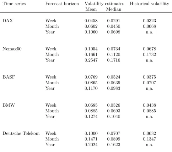
Table 2 presents means and medians of volatility estimates of our 106 experimental sub-jects concerning the five time series mentioned above over the forecast horizons of one week, one month, and one year. The table also shows historical volatilities that are the standard deviation of past weekly and monthly returns. Historical volatilities are often

used as an objective volatility benchmark or an estimate for the future volatility.21

Stan-19_{19 subjects answered on March 7, 39 subjects answered on March 8, 6 subjects answered on March 9, 6 subjects answered}

on March 10, 16 subjects answered on March 11, 11 subjects answered on March 12, 5 subjects answered on March 13, and

one subject answered on March 14, March 20, March 26, and April 3, respectively.

20_{See Pearson and Tukey (1965), p. 538.}

dard deviations of yearly returns are not shown due to the limited number of independent return observations in this case. The time periods for the calculation of standard deviation of returns are Jan 1, 1988 to December 31, 2003 (DAX, BASF, BMW), November 18, 1996 to December 31, 2003 (Deutsche Telekom), and January 1, 1998 to December 31, 2003 (Nemax50). The results appear quite reasonable. The longer the forecast horizon, the wider the confidence interval, i.e. the higher the volatility estimate. Furthermore, the volatility estimates for the three stocks (BASF, BMW, Deutsche Telekom) are higher than the volatility of the German large cap index DAX for all forecast horizons. All three stocks are part of the index. Thus, the index (usually) should have a lower volatility as the index is more diversified than a single stock that is part of the index.

The usual finding of studies analyzing stock market predictions is that subjects under-estimate the volatility of stock returns (usually measured by the standard deviation of past returns) indicating overconfidence (see, for example, Graham and Harvey (2002)). We find that this not true for short forecast horizons of one week. All one week volatility

estimates (apart from the median volatility estimate of the DAX) arehigher than

histor-ical volatilities. This is in line with Glaser and Weber (2005) who analyze stock return volatility forecasts of investors before and after the terror attacks of September 11. They find that in some cases, historical volatilities are overestimated.

In contrast, all median volatility estimates over a forecast horizon of one month are lower than historical volatilities indicating overconfidence.

However, Table 3 shows that focusing on means and medians hides considerable cross-sectional heterogeneity. As one example, Table 3 presents several percentiles of volatility estimates of our experimental subjects of the DAX over a one month forecast horizon.

This table shows that some investors strongly underestimate the variance of stock returns whereas other investors even overestimate historical volatilities.

To analyze as to whether the propensity to underestimate the variance of stock returns is a stable individual trait, we proceed as follows. We first calculate an overconfidence score for each investor and each volatility estimate by simply dividing 1 by the volatility estimate: OC_forecasti,k = 1 stddevk i (3) with stddevk

i as defined in equation (2).22 The higher OC_forecasti,k , the higher the degree

of overconfidence in stock market forecasts, i.e. the tighter the confidence interval. In the next step, we calculate pairwise correlation coefficients between these 15

over-confidence scores. All 105 correlation coefficients are highly significantly positive (p =

0.0000) with values between 0.2577 (corr(OC_forecastN emax50,W eek, OC_forecastT elekom,Y ear)) and 0.9163

(corr(OC_forecastBM W,M onth, OC_forecastBASF,M onth)). The average correlation is 0.6435 with a Cronbach

alpha of 0.9644.

To summarize, we find stable individual differences in the degree of overconfidence based on stock market forecasts.

22_{Another possibility is to define this overconfidence measure as 1−stddev}k

i or−stddevki. The results are similar when

we use these alternative definitions. Note that the alternative definitions do not affect the ranking of subjects according to

3.4 Trend Forecasting by Confidence Intervals

In this subsection, we present the results of a task that we refer to as “trend forecasting” or “trend prediction”. In this part of Study 1, experimental subjects observe artificially generated stock price charts which have, in the long run, either a positive or a negative trend. Subjects were asked to predict the future price development of these time-series charts via confidence intervals.

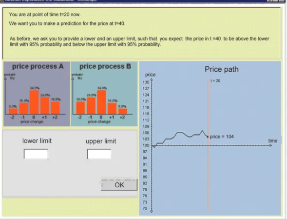
Subjects were confronted with two simple distributions of price changes (see Figure 1 for a

screenshot). Both processes could generate price movements of size−2,−1, 0, +1, and +2

with different probabilities. They were constructed such that one process had a positive trend, i.e. a positive expected value, and the other process had a negative trend. Both processes were graphically and numerically displayed. Subjects were further informed that one of the two processes was randomly picked to generate a price path. Three different pairs of price processes were used within the experiment. In all cases the distribution with positive trend is reflected at zero to obtain the distribution with negative trend. The following distributions were used:

Price movement (incremental change) −2 −1 0 +1 +2

D₁−_.5 = (18%, 24%, 34%, 16%, 8%) D+ 1.5 = (8%, 16%, 34%, 24%, 18%) D− 1.75 = (9.8%, 28%, 43%, 16%, 3.2%) D+ 1.75 = (3.2%, 16%, 43%, 28%, 9.8%) D− 2 = (12%, 32%, 37%, 16%, 3%) D+ 2 = (3%, 16%, 37%, 32%, 12%)

The index of Dk is chosen as the quotient of the probabilities for the outcome −1 and

the outcome +1. These odds k can be interpreted as a measure of the discriminability

of the two trends. In phase 2 of the experiment, for all subjects each process pair was used exactly once. Phase 3 was identical to phase 2 with different price paths presented

to subjects.23

After observing the chart until time t = 2024_{, subjects were asked to make a prediction}

about the price level at timet = 40. This judgment was elicited via a confidence interval,

consisting of an upper and lower limit. Subjects were instructed that the price at t = 40

should be above the upper limit and below the lower limit with 5 % probability each.

Thus, the stated confidence interval was supposed to contain the price at t= 40 with 90

% probability. These questions are similar to the knowledge questions and stock market predictions which we discussed in Subsections 3.1 and 3.3. The experimental subjects were asked to provide such confidence intervals for three price paths in phase 2 as well as in phase 3. Thus, we have six [low, high]-intervals overall, two for each of the price process

pairs D1.5,D1.75, and D2.25

For a given process pair Dk, the correct distribution of prices at t = 40 can be

com-puted from the price at t = 20 and the process distributions. Using this distribution,

the stated confidence intervals can be translated into intervals of probability percentiles 23_{To to be more explicit, the same overall set of price paths was used in both phases but with a different assignment}

across subjects.

24_{It should be noted that beforet= 20, subjects stated subjective probabilities that a given chart was generated by the}

distribution with the positive trend (which also determines their subjective probabilities that a chart was driven by the

process with the negative trend). See Glaser, Langer, and Weber (2003) for an extensive discussion and analysis of this task.

25_{Two professionals participated in only one of the two phases and thus provided only three intervals. We do not consider}

the results of phase 4 in this study as feedback about the performance in the earlier phases was given before the start of

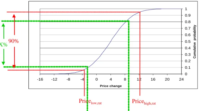
(see Figure 2 for a graphical illustration). For a perfectly calibrated subject these induced

probability intervals [plow%, phigh%] should be [5%, 95%].26 We measure the degree of

under-/overconfidence via the length of the induced probability interval. If a subject is too sure about the price at t=40 and provides a too narrow interval, it is classified as overconfident. More explicit, our measure of overconfidence in this task is defined as: OC_{trend prediction} = 90%−(phigh%−plow%) = 90%−x%. Positive OC_{trend prediction}

-values correspond to overconfidence, negative OC_{trend prediction}-values to

underconfi-dence. Figure 2 illustrates the calculation of the measurement of the degree of under-/overconfidence via the length of the induced probability interval.

In previous literature it was observed that individuals usually provide too narrow intervals

when making similar judgments.27_{The mean of the meanOC}

trend predictionmeasure per subject (across the three distributions used and the two phases considered) is 12.76 % (the median is 18.44 %) indicating overconfidence. Thus, our experimental subjects state confidence intervals that are, on average, about 13 percentage points too narrow. We can

comfortably reject the hypothesis that the OC_{trend prediction} measure is equal to zero

(p < 0.0001). Again, focusing on means and medians alone hides large cross-sectional

heterogeneity. For example, 23 subjects show aOC_{trend prediction}measure that is larger

than 35. To further investigate the issue of stable individual differences, we first calculate

the meanOC_{trend prediction} per distribution. We thus obtain three OC_{trend prediction},

one per each k. The correlation coefficients are highly significantly positive (all p-values

are lower than 0.0001) with values between 0.8006 and 0.8730 and an average of 0.8329. The Cronbach alpha is 0.9373.

26_{Note, however, that due to the discreteness of the distribution it was not possible in general to exactly hit this target.}

3.5 Stability over Time

For the task described in the previous subsection, we are able to analyze the stability over time as the task was fulfilled in phase two and in phase three. There was a lag of about two weeks between these two tasks.

The correlation of the overconfidence measureOC_{trend prediction}between phase two and

phase three is 0.7055 (p < 0.0001). The overconfidence measure is calculated as follows.

In each phase, we calculate the mean OC_{trend prediction} score per each subject in each

time period across the three odds. The correlation presented above is highly significantly positive suggesting stability over time. We are thus able to confirm results of Jonsson and Allwood (2003) who find stability over time for the concept of miscalibration.

4

Results: Individual Differences Between Tasks?

4.1 The Correlation of Overconfidence Scores Between Tasks

In this subsection we analyze individual differences in the degree of judgment biases across several tasks by calculating correlation coefficients. Table 4 summarizes the overconfidence measures we defined in the two studies.

Table 5 presents the results on the correlation coefficients between the overconfidence

scores across several tasks separately for Study 1 and Study 2.28 _{Most of the correlations}

are highly significantly positive. Some correlations are negative but insignificant. The strongest result is that overconfidence scores based on confidence interval questions are 28_{The results are similar when we calculate the correlations in Study 2 separately for the Frankfurt and the London group.}

highly significantly positive. This is surprising as we measure the degree of miscalibration using confidence intervals in distinct time periods and across a very heterogeneous subject pool. Furthermore, we asked for confidence intervals in different domains (knowledge questions, real world financial time series, artificially generated time series). Thus, we are able to confirm studies showing that individual differences are especially strong when subjects are asked to state subjective confidence intervals (see, for example, Klayman, Soll, Gonz´ales-Vallejo, and Barlas (1999), p. 240).

The correlation between OC_{better than others} and other overconfidence scores is mainly

insignificant or even significantly negative. This finding is consistent with other studies that also analyze the correlation between miscalibration and the better than others (or better than average) effect. Glaser and Weber (2004) find that most of the correlations between their miscalibration scores and their better than average scores are insignificant. Deaves, L¨uders, and Luo (2003) measure miscalibration and the better than average ef-fect using essentially the same questions as Glaser and Weber (2004) do. The correlation matrix in the Deaves, L¨uders, and Luo (2003) study shows no significant positive correla-tions between these scores. Oberlechner and Osler (2003) find a negative (but statistically and economically insignificant) correlation between miscalibration and the better than average effect. R´egner, Hilton, Cabantous and Vautier (2004) find little or now correla-tion between miscalibracorrela-tion, positive illusions such as unrealistic optimism, and a general tendency to consider oneself as better than average. These findings do not coincide with conjectures that miscalibration and the better than average effect are related.

4.2 Traders Versus Students

To further analyze the issue of stable individual differences across tasks, we analyze whether the degree of overconfidence is different across several subject pools. To be more specific, we analyze whether professionals are more biased or whether the experience of professionals mitigates the degree of a judgment bias. We are thus able to contribute to

the literature on expert judgment.29

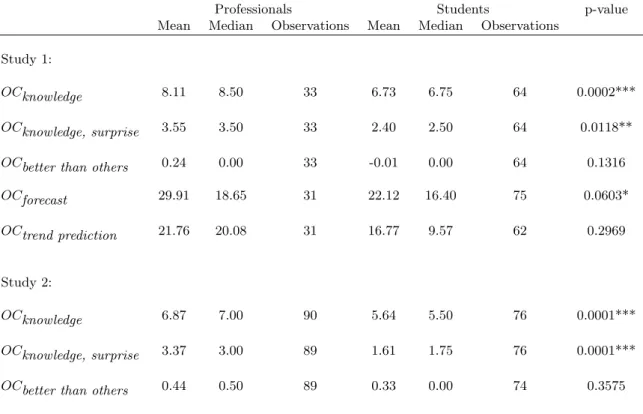
Table 6 presents means and medians of the overconfidence measures summarized in Table 4 for professionals and students as well as the number of observations in the two studies.

The last column contains p-values of a Kruskal-Wallis test. Null hypothesis is equality

of populations. In both studies, all scores of professionals are higher than the respective

scores of students. In most cases this result is significant. We are thus able to confirm studies that show a higher degree of a bias among professionals compared to students (see, for example, Haigh and List (2005)).

5

Discussion and Conclusion

In our study, we analyze whether professionals (traders who work in the trading room of a large bank; investment bankers) are subject to judgment biases to the same degree as a population of students. We examine whether there are individual differences in the degree of overconfidence within various specific task. Furthermore, we analyze whether the degree of judgment biases is correlated across tasks, i.e. whether the same individuals are more biased in their judgments than others in a variety of domains. Professionals and

a student control group participated in a multi-task experiment that was (for participants of Study 1) in part conducted via the internet. Our data enables us to measure the degree of overconfidence in various dimensions, to analyze whether there are stable individual differences in the degree of overconfidence within several distinct tasks, and to investigate whether the degree of overconfidence is correlated across tasks.

Our main results can be summarized as follows. Judgments of professionals are biased. In all tasks and in both studies, their degrees of overconfidence are higher than the respective scores of the student control group. In most tasks, this difference is significant. In line with extant literature, we find stable individual differences within tasks (e.g. in the degree of miscalibration, as measured by confidence interval questions). However, we find that correlations across distinct tasks are sometimes insignificant or even negative. We are thus able to confirm some preliminary results in the literature.

Our results are important for several reasons. It is often argued that not much can be learned from experiments with a student subject about real-world financial markets be-cause professional investors have a much higher influence or price impact than individual investors and are thus more important in the process of determining market allocations and market outcomes. We show that professionals are biased even in job related tasks such as forecasting real world financial time series. Therefore, expertise does not miti-gate biases. Moreover, our results concerning stable individual differences within tasks strengthen the common modeling assumption in finance that investors with different de-grees of overconfidence can be regarded as different investor types.

Furthermore, we find simultaneous over- and underconfidence. According to the knowl-edge calibration questions, all investors are overconfident, whereas in other tasks some

subjects can be classified as underconfident (for example in the stock market forecast task). Kirchler and Maciejovsky (2002) find similar results. They investigate individual overconfidence in the context of an experimental asset market with several periods. Be-fore each period, overconfidence was measured. Participants were asked to state subjective confidence intervals for the price of the single risky asset in the next trading period as well as their subjective certainty. They also find simultaneous over- and underconfidence. Depending on the method (subjective confidence intervals on the one hand and the com-parison of objective accuracy and subjective certainty on the other) overconfidence was measured some participants can be classified as either overconfident or underconfident. One interpretation might be that people show different levels of overconfidence depending on the task or domain but the same rank-order over tasks or domains. Our results and the results of Jonsson and Allwood (2003), p. 561, and Glaser and Weber (2004) suggest that this might be the case. Furthermore we argue that some facets of overconfidence that are often assumed to be related (miscalibration and the better than others effect) are actually unrelated which casts doubt on the optimistic overconfidence perspective as a framework for explaining judgmental overconfidence.

References

Alba, J. W., and J. W. Hutchinson, 2000, “Knowledge Calibration: What Consumers

Know and What They Think They Know,” Journal of Consumer Research, 27, 123–

156.

Benos, A. V., 1998, “Aggressiveness and survival of overconfident traders,” Journal of

Financial Markets, 1, 353–383.

Biais, B., D. Hilton, K. Mazurier, and S. Pouget, 2005, “Judgemental overconfidence,

self-monitoring and trading performance in an experimental financial market,” Review

of Economic Studies, 72, 287–312.

De Bondt, W. F., 1998, “A portrait of the individual investor,” European Economic

Re-view, 42, 831–844.

Deaves, R., E. L¨uders, and R. Luo, 2003, “An Experimental Test of the Impact of Over-confidence and Gender on Trading Activity,” Working paper, McMaster University. Gigerenzer, G., 1991, “How to make cognitive illusions disappear: Beyond “heuristics and

biases”,” in W. Stroebe, andM. Hewstone (ed.), European Review of Social Psychology,

Vol. 2 pp. 83–115.

Glaser, M., T. Langer, and M. Weber, 2003, “On the Trend Recognition and Forecasting Ability of Professional Traders,” CEPR Discussion Paper DP 3904.

Glaser, M., M. N¨oth, and M. Weber, 2004, “Behavioral Finance,” in Derek J. Koehler,and

Nigel Harvey (ed.),Blackwell Handbook of Judgment and Decision Making, pp. 527–546,

Glaser, M., and M. Weber, 2004, “Overconfidence and Trading Volume,” Working paper, University of Mannheim.

Glaser, M., and M. Weber, 2005, “September 11 and Stock Return Expectations of

Indi-vidual Investors,” Review of Finance, 9, –, forthcoming.

Graham, J. R., and C. R. Harvey, 2002, “Expectations Of Equity Risk Premia, Volatility, And Asymmetry,” Working Paper, Duke University.

Griffin, D., and L. Brenner, 2004, “Perspectives on Probability Judgment Calibration,” in

Derek Koehler, and Nigel Harvey (ed.), Blackwell Handbook of Judgment and Decision

Making, pp. 177–199, Blackwell.

Haigh, M. S., and J. A. List, 2005, “Do Professional Traders Exhibit Myopic Loss

Aver-sion? An Experimental Analysis,” Journal of Finance, 60, 523–534.

Hilton, D. J., 2001, “The Psychology of Financial Decision-Making: Applications to

Trad-ing, DealTrad-ing, and Investment Analysis,” Journal of Psychology and Financial Markets,

2, 37–53.

Jonsson, A.-C., and C. M. Allwood, 2003, “Stability and variability in the realism of

con-fidence judgments over time, content domain, and gender,” Personality and Individual

Differences, 34, 559–574.

Keefer, D. L., and S. E. Bodily, 1983, “Three-Point Approximations for Continuous

Ran-dom Variables,” Management Science, 29, 595–609.

Kilka, M., and M. Weber, 2000, “Home Bias in International Stock Return Expectations,” Journal of Psychology and Financial Markets, 1, 176–192.

Kirchler, E., and B. Maciejovsky, 2002, “Simultaneous over- and underconfidence:

Evi-dence from experimental asset markets,” Journal of Risk and Uncertainty, 25, 65–85.

Klayman, J., J. B. Soll, C. Gonz´ales-Vallejo, and S. Barlas, 1999, “Overconfidence: It

Depends on How, What, and Whom You Ask,” Organizational Behavior and Human

Decision Processes, 79, 216–247.

Koehler, D. J., L. Brenner, and D. Griffin, 2002, “The calibration of expert judgment:

Heuristics and biases beyond the laboratory,” in Thomas Gilovich, Dale Griffin, and

Daniel Kahneman (ed.), Heuristics and Biases: The Psychology of Intuitive Judgment,

pp. 489–509, Cambridge University Press.

Langer, E. J., 1975, “The Illusion of Control,”Journal of Personality and Social

Psychol-ogy, 32, 311–328.

Lichtenstein, S., B. Fischhoff, and L. D. Phillips, 1982, “Calibration of probabilities: The

state of the art to 1980,” in Daniel Kahneman, Paul Slovic, and Amos Tversky (ed.),

Judgment under uncertainty: Heuristics and Biases, pp. 306–334, Cambridge University Press.

Locke, P. R., and S. C. Mann, 2000, “Do Professional Traders Exhibit Loss Realization Aversion?,” Working paper, George Washington University and Texas Christian Uni-versity.

L¨offler, G., and M. Weber, 1997, “Welche Faktoren beeinflussen erwartete Aktienrenditen?

- eine Analyse anhand von Umfragedaten,” Zeitschrift f¨ur Wirtschafts- und

Sozialwis-senschaften, 117, 209–246.

Oberlechner, T., and C. L. Osler, 2003, “Overconfidence in Currency Markets,” Working paper.

Odean, T., 1998, “Volume, Volatility, Price, and Profit When All Traders Are Above

Average,” Journal of Finance, 53, 1887–1934.

Pallier, G., R. Wilkinson, V. Danthiir, S. Kleitman, G. Knezevic, L. Stankov, and R. D. Roberts, 2002, “The Role of Individual Differences in the Accuracy of Confidence

Judg-ments,” Journal of General Psychology, 129, 257–299.

Parker, A. M., and B. Fischhoff, 2001, “Decision-Making Competence: An Individual-Differences Approach,” Working paper.

Person, E., and J. Tukey, 1965, “Approximate Means and Standard Deviations Based on

Distances between Percentage Points of Frequency Curves,” Biometrika, 52, 533–546.

Presson, P. K., and V. A. Benassi, 1996, “Illusion of Control: A Meta-Analytic Review,” Journal of Social Behavior and Personality, 11, 493–510.

R´egner, I., D. Hilton, L. Cabantous, and S. Vautier, 2004, “Overconfidence, Miscalibration and Positive Illusions,” Working paper, University of Toulouse.

Russo, J. E., and P. J. H. Schoemaker, 1992, “Managing Overconfidence,” Sloan

Manage-ment Review, 33, 7–17.

Siebenmorgen, N., and M. Weber, 2004, “The Influence of Different Investment Horizons

on Risk Behavior,” Journal of Behavioral Finance, 5, 75–90.

Soll, J. B., 1996, “Determinants of overconfidence and miscalibration: The roles of

ran-dom error and ecological structure,” Organizational Behavior and Human Decision

Soll, J. B., and J. Klayman, 2004, “Overconfidence in Interval Estimates,” Journal of Experimental Psychology: Learning, Memory, and Cognition, 30, 299–314.

Stanovich, K. E., and R. F. West, 1998, “Individual differences in Rational Thought,” Journal of Experimental Psychology, 127, 161–188.

Stanovich, K. E., and R. F. West, 2000, “Individual differences in reasoning: Implications

for the rationality debate,” Behavioral and Brain Sciences, 23, 645–726.

Svenson, O., 1981, “Are we all less risky and more skillful than our fellow drivers?,”Acta

Psychologica, 47, 143–148.

Taylor, S. S., and J. D. Brown, 1988, “Illusion and well being: A social psychology

per-spective on mental health,” Psychological Bulletin, 103, 193–210.

Weinstein, N. D., 1980, “Unrealistic Optimism About Future Life Events,” Journal of

Table 1:Overconfidence in Knowledge Questions: Results

This table presents the mean, minimum, maximum, and several percentiles of the number of correct answers that fall outside the 90 % confidence interval for general knowledge questions as well as eco-nomics and finance knowledge questions, respectively given by our experimental subjects in study 1. See Subsection 3.1 for details.

General knowledge Banking and finance knowledge

Number of observations 97 97 Mean 6.60 7.80 Minimum 2 3 5th percentile 3 5 10th percentile 4 5 25th percentile 5 7 Median 7 8 75th percentile 8 9 90th percentile 9 10 95th percentile 10 10 Maximum 10 10

Table 2:Volatility Estimates

This table presents means and medians of volatility estimates of 106 experimental subjects in study 1 (31 professionals, 75 students) of five time series over three forecast horizons (one week, one month, and one year). Volatility estimates are calculated as described in Subsection 3.3. The table also shows historical volatilities that are the standard deviation of past weekly and monthly returns. Standard deviations of yearly returns are not shown due to the limited number of independent return observations in this case. The time periods for the calculation of standard deviation of returns are Jan 1, 1988 to December 31, 2003 (DAX, BASF, BMW), November 18, 1996 to December 31, 2003 (Deutsche Telekom), and January 1, 1998 to December 31, 2003 (Nemax50).

Time series Forecast horizon Volatility estimates Historical volatility Mean Median DAX Week 0.0458 0.0291 0.0323 Month 0.0602 0.0450 0.0668 Year 0.1060 0.0698 n.a. Nemax50 Week 0.1054 0.0734 0.0678 Month 0.1661 0.1120 0.1732 Year 0.2547 0.1716 n.a. BASF Week 0.0769 0.0524 0.0375 Month 0.0865 0.0639 0.0707 Year 0.1170 0.0983 n.a. BMW Week 0.0685 0.0526 0.0438 Month 0.0885 0.0693 0.0885 Year 0.1274 0.1040 n.a.

Deutsche Telekom Week 0.1000 0.0707 0.0632 Month 0.1471 0.0899 0.1347

Table 3:DAX Volatility Estimates: Individual Differences

This table presents several percentiles of volatility estimates of 106 experimental subjects in study 1 (31 professionals, 75 students) of the DAX over a one month forecast horizon. Volatility estimates are calculated as described in Subsection 3.3. The table also shows the historical standard deviation of monthly DAX returns. The time period for the calculation of the standard deviation of returns is Jan 1, 1988 to December 31, 2003. Volatility estimate 5th percentile 0.0115 10th percentile 0.0116 25th percentile 0.0287 Median 0.0450 75th percentile 0.0814 90th percentile 0.1163 95th percentile 0.1454 Historical volatility 0.0668

T able 4: Summary of Ov erconfidence Measures This table summarizes and defines ov erconfidence scores used in Section 4. Ov erconfidence measure Description O Cknow le dge Av erage of tw o ov erconfidence scores based on general kno wledge and economics and finance kno wledge confidence in terv al questions (see Subsection 3.1). O Cknow le dge, surprise Ov erconfidence score based on the comparison b et w een the actual and exp ected n um b er of surprises in confidence in terv al (see Subsection 3.1). O Cbetter than others Ov erconfidence score based on the comparison b et w een assessmen t of own p erformance in kno wledge questions and p erformance of others (see Subsection 3.2). O Cfor ec ast Av erage of ov erconfidence scores based on sto ck mark et forecasts (see Subsection 3.3) O Ctr end pr ediction Ov erconfidence score based on trend prediction b y confidence in terv als (see Subsection 3.4).

T able 5: Individual Differences Bet w een T asks: The Correlation of Ov erconfidence Scores This table presen ts pairwise correlation co efficien ts b et w een the ov erconfidence measures summarized and defined in T able 4 as w ell as the significance lev el of eac h correlation co efficien t (in paren theses) and the n um b er of observ ations used in calculating the correlation co efficien t separately for study 1 and study 2. ** indicates significance at 5%; *** indicates significance at 1%. O Cknow le dge O Cknow le dge, surprise O Cbetter than others O Cfor ec ast O Ctr end pr ediction Study 1: O Cknow le dge 1.0000 97 O Cknow le dge, surprise 0.4653 1.0000 (0.0000)*** 97 97 O Cbetter than others -0.1397 0.2394 1.0000 (0.1725) (0.0182)** 97 97 97 O Cfor ec ast 0.2963 0.2252 -0.0543 1.0000 (0.0035)*** (0.0282)** (0.6015) 95 95 95 106 O Ctr end pr ediction 0.5363 0.3122 0.0766 0.5242 1.0000 (0.0000)*** (0.0025)*** (0.4679) (0.0000)*** 92 92 92 93 93 Study 2: O Cknow le dge 1.0000 166 O Cknow le dge, surprise 0.5815 1.0000 (0.0000)*** 165 165 O Cbetter than others -0.1812 0.2708 1.0000 (0.0206)** (0.0005)*** 163 163 163

Table 6:Individual Differences Between Tasks: Professionals versus Students

This table presents means and medians of the overconfidence measures summarized in Table 4 for profes-sionals and students as well as the number of observations separately for study 1 and study 2. The last column containsp-values of a Kruskal-Wallis test. Null hypothesis is equality of populations. * indicates significance at 10%; **indicates significance at 5% ***; indicates significance at 1%.

Professionals Students p-value Mean Median Observations Mean Median Observations

Study 1:

OC_knowledge 8.11 8.50 33 6.73 6.75 64 0.0002***

OC_{knowledge, surprise} 3.55 3.50 33 2.40 2.50 64 0.0118**

OC_{better than others} 0.24 0.00 33 -0.01 0.00 64 0.1316

OC_forecast 29.91 18.65 31 22.12 16.40 75 0.0603*

OC_{trend prediction} 21.76 20.08 31 16.77 9.57 62 0.2969 Study 2:

OC_knowledge 6.87 7.00 90 5.64 5.50 76 0.0001***

OC_{knowledge, surprise} 3.37 3.00 89 1.61 1.75 76 0.0001***

Figure 2: Measurement of the Degree of Under-/Overconfidence via the Length of the In-duced Probability Interval

0 0.1 0.2 0.3 0.4 0.5 0.6 0.7 0.8 0.9 1 -16 -12 -8 -4 0 4 8 12 16 20 24 Price change C u m u la ti v e p ro b a b il it y

X%

Price

Price

90%

SONDERFORSCHUNGSBereich

504

Overconfidence of Professionals and Lay Men: Individual Differences Within and Between Tasks?

05-24 Volker Stock´e Determinanten und Konsequenzen von

Nonresponse in egozentrierten Netzwerkstudien 05-23 Lothar Essig Household Saving in Germany: Results from SAVE

2001-2003

05-22 Lothar Essig Precautionary saving and old-age provisions: Do subjective saving motives measures work?

05-21 Lothar Essig Imputing total expenditures from a non-exhaustive list of items: An empirical assessment using the SAVE data set

05-20 Lothar Essig Measures for savings and saving rates in the German SAVE data set

05-19 Axel B¨orsch-Supan Lothar Essig

Personal assets and pension reform: How well prepared are the Germans?

05-18 Lothar Essig Joachim Winter

Item nonresponse to financial questions in household surveys: An experimental study of interviewer and mode effects

05-17 Lothar Essig Methodological aspects of the SAVE data set 05-16 Hartmut Esser Rationalit¨at und Bindung. Das Modell der

Frame-Selektion und die Erkl¨arung des normativen Handelns

05-15 Hartmut Esser Affektuelles Handeln: Emotionen und das Modell der Frame-Selektion

05-14 Gerald Seidel Endogenous Inflation - The Role of Expectations and Strategic Interaction

05-13 Jannis Bischof Zur Fraud-on-the-market-Theorie im US-amerikanischen informationellen

Kapitalmarktrecht: Theoretische Grundlagen, Rechtsprechungsentwicklung und Materialien

SONDERFORSCHUNGSBereich

504

Nr. Author Title

2

05-12 Daniel Schunk Search behaviour with reference point preferences: Theory and experimental evidence

05-11 Clemens Kroneberg Die Definition der Situation und die variable Rationalit¨at der Akteure. Ein allgemeines Modell des Handelns auf der Basis von Hartmut Essers Frame-Selektionstheorie

05-10 Sina Borgsen Markus Glaser

Diversifikationseffekte durch Small und Mid Caps? Eine empirische Untersuchung basierend auf europ¨aischen Aktienindizes

05-09 Gerald Seidel Fair Behavior and Inflation Persistence 05-08 Alexander Zimper Equivalence between best responses and

undominated strategies: a generalization from finite to compact strategy sets.

05-07 Hendrik Hakenes Isabel Schnabel

Bank Size and Risk-Taking under Basel II

05-06 Thomas Gschwend Ticket-Splitting and Strategic Voting under Mixed Electoral Rules: Evidence from Germany

05-05 Axel B¨orsch-Supan Risiken im Lebenszyklus: Theorie und Evidenz 05-04 Franz Rothlauf

Daniel Schunk Jella Pfeiffer

Classification of Human Decision Behavior: Finding Modular Decision Rules with Genetic Algorithms

05-03 Thomas Gschwend Institutional Incentives for Strategic Voting: The Case of Portugal

05-02 Siegfried K. Berninghaus Karl-Martin Ehrhart Marion Ott

A Network Experiment in Continuous Time: The Influence of Link Costs

05-01 Gesch¨aftsstelle Jahresbericht 2004

04-70 Felix Freyland Household Composition and Savings: An Empirical Analysis based on the German SOEP data