QUT Digital Repository:
http://eprints.qut.edu.au/
Yu, Yi and Ma, Lin and Gu, YuanTong and Zhou, Yifan (2008) Confidence interval of lifetime distribution using bootstrap method. In: The Third World Congress on Engineering Asset Management and Intelligent Maintenance Systems Conference, 27-30 October 2008, Beijing, China.
©
Copyright 2008 Springer
This is the author-version of the work. Conference proceedings published, by Springer Verlag, will be available via SpringerLink.
CONFIDENCE INTERVAL OF LIFETIME DISTRIBUTION USING BOOTSTRAP
METHOD
Yi Yu a, b, Lin Ma a, b, Yuantong Gu b, Yifan Zhou a, b
a
Cooperative Research Centre for Integrated Engineering Asset Management (CIEAM)
b School of Engineering Systems, Faculty of Built Environment and Engineering, Queensland University of Technology,
Brisbane, Australia
Lifetime estimation is significant in engineering asset management. However, the estimate of lifetime or failure time could be misleading as it may not reveal the real value. Therefore, confidence intervals need to be built to quantify the prediction uncertainty. For the Gamma process, which is a commonly used method for lifetime estimation, the conventional confidence interval construction methods do not perform well. This paper adopts bootstrap methods to build confidence intervals of lifetime distribution when the Gamma process is used. Three bootstrap methods, i.e. bootstrap percentile, bootstrap-t and bootstrap bias corrected & accelerated (BCa), are utilized and investigated. These methods are first applied to the basic Gamma process and further to the Gamma process which considers random effects. Moreover, bootstrap calibration is conducted to assess the coverage probability of the confidence intervals built by these bootstrap methods. Applications to the fatigue crack growth data are carried out as a case study. The results show that the BCa method is recommended for generating confidence intervals for Gamma processes in this application.
Key Words: Bootstrap Methods, Confidence Intervals, Gamma Process, Degradation Model
1 INTRODUCTION
In recent years, much attention has been given to the deterioration of engineering assets. Many methods have been proposed to model the deterioration process. One of the commonly used approaches to model asset degradation processes is the Gamma process, in which increments over time follow Gamma distributions. A Gamma process possesses the feature of both a Markovian and a jump process. This combined feature makes it attractive to reliability analysts as it can model both slow continuous deterioration and shocks in the process.
The prediction results of a Gamma degradation model can be presented by a point-wise estimation value and the corresponding confidence intervals. Obviously, analytical results would be less convincing and even doubtful without identifying the prediction uncertainty. The commonly used approach for generating a confidence interval is the asymptotic normal approximation, which only performs well when the sample size is large enough. Another obstacle to applying asymptotic normal approximation in Gamma degradation estimations is the complexity of obtaining derivatives of quantities of interest with respect to the Gamma process parameters [1]. Other confidence interval estimation methods, such as the likelihood ratio test[2]may give better interval estimates. However the computational complexity makes it less competitive.
These obstacles stimulate the need for methods which are able to handle a small sample situation, and also can provide intervals with coverage probability equal or close to the nominal value. Bootstrapping method [3], a re-sampling approach for statistical inference, is capable of dealing with small-size samples with high accuracy. In this paper, the bootstrap theory is employed to obtain confidence intervals for Gamma degradation analyses. Three bootstrap methods are applied and investigated. Their coverage probability and performance are also studied through the comparison among these methods.
The rest parts of this paper are organised as follows: Section 2 introduces the lifetime distributions based on the Gamma processes. Section 3 describes how to use three bootstrap methods to generate confidence intervals for these lifetime distributions. Section 4 presents the bootstrap calibration to examine the coverage accuracy of the estimated intervals. A case study using a degradation sample from Hudak, Saxena et al. [4] is conducted in Section 5, where case study results are also analysed and findings are drawn based on the analyses. Section 6 presents the conclusion of this paper.
2 THE LIFETIME DISTRIBUTION BASED ON GAMMA PROCESSES
2.1 The Basic Gamma Process
A Gamma process is a continuous stochastic process with independent Gamma-distributed increments. Considering the non-decreasing Gamma process
{ ( ),
x t t
≥
0}
, when applied to a degradation process,x t
( )
represents the measured degradation at timet
.The probability density function for increments is defined by
=
∆
∆
;
,
)
(
x
iα
t
iβ
f
1exp(
/ )
(
)
i i t i i t ix
x
t
α αβ
α
β
∆ − ∆∆
−∆
Γ ∆
(1)Where
∆ =
x
i[ ( )
x t
i−
x t
(
i−1), ( )
x t
0=
0]
is the degradation increments,∆
t
i=
(
t
i−
t
i−1,
t
0=
0
)
is the time increments,α
∆
t
i andβ
are called shape and scale parameters of the basic Gamma process, andds
e
s
u
=
∫
∞ u− −sΓ
0 1)
(
is the gamma function.The parameters of the Gamma process are often estimated by maximizing the log-likelihood function of degradation increments. The likelihood function is a product of the independent probability density functions, therefore:
1 1 2,..., 1 1
(
,
)
(
)
exp(
/ )
(
)
i i t n n i n i t i i i ix
L
x
x
x
f
x
x
t
α αβ
α
β
∆ − ∆ = =∆
∆ ∆
∆
=
∆ =
−∆
Γ ∆
∏
∏
(2) Differentiating the logarithm form of the likelihood function with respect toα
andβ
, we have maximum likelihood estimates satisfying[5]: ^ ^ n nx
t
β
α
=
, ^ ^ 1[log
(
)]
log
n n i i i n i nx
t
x
t
t
t
ψ α
α
=∆
∆ −
∆
=
∑
(3)In which
x
n andt
n stand for∑
=
∆
n
i 1
x
i and∑
=∆
n
i 1
t
irespectively, andψ
represents the digamma function, thederivative of log Gamma function.
In the degradation analysis, a failure is said to have occurred when the deterioration process first passes a pre-determined level
s
.s
is called the degradation threshold. Defining the lifetime asT
, according to the monotonically increasing Gamma degradation process, the cumulative distribution function of lifetime [5]:( / ,
)
( )
Pr(
)
Pr{ ( )
}
(
)
Ts
t
F t
T
t
x t
s
t
β α
α
Γ
=
< =
≥ =
Γ
(4) Here( , )
y 1 z xx y
∞z
− −e dz
Γ
=
∫
(x
>
0,
y
≥
0
) is the incomplete Gamma function.2.2 Gamma Processes Considering Random Effects
In the case of basic Gamma process, the scale parameter is treated as a constant. However, this does not necessarily mean that the scale parameter has to be fixed. The basic Gamma process can be extended by letting
β
change with time or follow a certain distribution. In particular, setting the scale parameterβ
follow an inverse Gamma distribution, i.e.β
−1~
Ga
( ,
δ γ
−1)
, the extended Gamma process is suitable for considering random effects involved in the asset degradation process [1]. Now the heterogeneity in degradation paths can be modelled by the variation among the scale parameters.For processes with random effects, the degradation increments are not always independent. The independence of the increments of a single sample path is conditional on the common random effect, i.e. the same
β
. Now the likelihood function is: 1 1 1 2,..., 1(
,
)
( ; ,
)
(
;
,
)
n n i i iL
x
x
x
f
κ δ γ
−f
x
α
t
κ
−d
κ
=∆ ∆
∆
=
∫
∏
∆
∆
1 1 1(
)
(
)
( )
(
)
i n n t i n i n t n i ix
t
x
t
α δ δ αγ
δ α
γ
δ
α
∆ − = + =∆
Γ +
=
+
Γ
Γ ∆
∏
∏
(5)According to [1], the lifetime distribution for the random effect degradation process can be described by a F distribution:
( )
Pr(
)
Pr( ( )
) 1
(
; 2
, 2 )
Ts
F t
T
t
X t
s
F
t
t
δ
α δ
γα
=
< =
≥ = −
(6)3 BOOTSTRAP METHODS FOR CALCULATION OF LIFETIME DISTRIBUTION CONFIDENCE INTERVALS
Bootstrap methods are one type of re-sampling approaches. The basic theory of bootstrapping is: Suppose
S
is a function of random variables depending on the parameterθ
, the parametric bootstrap versionS
*ofS
is calculated using the bootstrap samples simulated using^
θ
, the estimate ofθ
[6].Three bootstrap methods are studied here. These are bootstrap percentile, bootstrap-t method and bootstrap bias corrected and accelerated (BCa) method. A brief description of these three methods is given first. Then we will propose the detailed procedures for bootstrap application in Gamma degradation analyses.
Suppose
* ^
θ
is an estimate computed from a bootstrap data sample. Let* ^
p
θ
be the p-th percentile of the distribution of* ^
θ
, an approximate 100*(1-p
)% bootstrap percentile confidence interval forθ
is determined by^ * / 2 p
θ
and ^ * 1 p/ 2θ
− .For the bootstrap-t method, considering the bootstrap distribution of transformation
^ ^ ^ ^ * *
(
θ θ
−
) /
se
( )
θ
with ^ ^ *( )
se
θ
the bootstrap version of ^ ^( )
se
θ
, the k-th percentile for this distribution is defined as ^ * kz
θ
. The bootstrap-t confidence interval is
[ ^* 1 / 2 ^ ^ ^
( )
pz
se
θθ
θ
−−
, ^* / 2 ^ ^ ^( )
pz
se
θθ
−
θ
][7] [8].In order to offset the possible bias in
^
θ
, the estimate calculated from original sample, theBC
a method has been proposed[8, 9]. The bootstrapBC
a100*(1-p
)% confidence interval is given by1 ^ * p
θ
and 2 ^ * pθ
,p
1andp
2aredetermined using the equations below:
^ ^ 0 / 2 1 0 ^ ^ 0 / 2
(
)
1
(
)
p pz
z
p
z
a z
z
+
= Φ +
−
+
and ^ ^ 0 1 / 2 2 0 ^ ^ 0 1 / 2(
)
1
(
)
p pz
z
p
z
a z
z
− −+
= Φ +
−
+
(7) ^ 0z
anda
are called bias-correction and acceleration respectively [8, 9].3.1 Lifetime Distribution Interval Calculation Using Bootstrap Methods
The bootstrap methods described above are applied to both the basic Gamma process and the Gamma process considering random effects to get intervals for lifetime distribution. For the basic Gamma process, there are several steps involved, which are listed as follows:
Step 1. Estimate the Gamma process parameter
α
andβ
from the degradation sample paths using equation (3), inserting the estimates^
α
and^
β
to (4) to obtain lifetime distribution estimate^
( )
TF
t
;Step 2. Generate
B
bootstrap samples from the Gamma process function (1) using the estimated parameters^
α
and^
β
;Step 3. For the
i
-th Bootstrap sample, parameters are estimated again as (* ^ i
α
, * ^ iβ
) and further the bootstrap estimates * ^( )
T iF
t
;Step 4. With different bootstrap methods, 100*(1-
p
)% bootstrap confidence intervals for the lifetime distribution^
( )
TF
t
are calculated differently:
1) The percentile bootstrap confidence interval is [
* ^ / 2
( )
T pF
t
, * ^ 1 / 2( )
T pF
t
− ], where * ^ / 2( )
T pF
t
and * ^ 1 / 2( )
T pF
t
− are the*
/ 2
B p
-th andB
* (1
−
p
/ 2)
-th ordered values of* ^
( )
T i
F
t
;2) The bootstrap-t confidence interval can be described as [
^ ^ ^ ^ ^ ^ 1 / 2 / 2
( )
p*
,
( )
p*
T TF
t
−
Z
−se F
t
−
Z
se
], ^ / 2 pZ
and ^ 1 p/ 2Z
− are the orderedB p
*
/ 2
-th andB
* (1
−
p
/ 2)
-th values of* * ^ ^ ^ *
(
( )
( )) /
i T i T FZ
=
F
t
−
F t
se
respectively. 3) When applying the bootstrap BCa method, the lower and upper endpoints of 100*(1-p
)% confidence interval for thelifetime distribution are the ordered
B p
*
1-th andB p
*
2-th values of the* ^
( )
T i
F
t
, wherep
1andp
2are calculated by(7), the bias correction parameter
{#
[
(
)
(
)]
/
}
^ * ^ 1 ^ 0
F
t
F
t
B
z
=
Φ
− T i≤
T (#[
Function
]
calculates the number of times that the Function would be satisfied) and acceleration parameter^ ^ ^ ^ ^ 3 2 3/ 2 (.) ( ) (.) ( ) 1
(
) / 6{
1(
) }
n n i i i ia
F
F
F
F
= ==
∑
−
∑
−
, in which ^ ( )iF
is the lifetime distribution estimate obtained using the original sample without thei
-th value and^ (.)
F
is the average of ^ ( )iF
(1≤ ≤
i
n
).For processes with the random effects, the algorithm is quite similar to that of basic Gamma Processes. The parameter estimates are ^
α
, ^δ
and ^γ
, which can be gained through the maximization of equation (5). Another difference is that lifetime distributionF
T( )
t
is determined by (6) rather than (4).4 THE COVERAGE ACCURACY OF BOOTSTRAP CONFIDENCE INTERVALS
It is important to examine the coverage probability of calculated confidence intervals. If the exact interval with the nominal coverage probability is known, the evaluation of estimated confidence intervals would be straightforward. However, the
nominal interval is usually unknown or difficult to calculate. Therefore, the coverage errors of calculated confidence intervals have to be estimated. One interesting feature of bootstrapping is that it can also be used for this purpose[3, 10, 11]. The application is called bootstrap calibration, which assesses and improves the coverage accuracy of approximate confidence intervals, including the intervals constructed by bootstrapping.
The bootstrapping for the confidence interval calibration can be described as follows [3]:
Define
[
]
^
u
θ
the estimatedu
-level upper endpoint of the one sided confidence interval forθ
, the interval is supposed to have the nominal coverage probability, which means[
]
^
u
θ
satisfyingPr(
≤
[
u
])
=
u
^θ
θ
is preferred.In reality, however, the actual coverage of a confidence interval is seldom equal to the nominal value. Generally we define
v
u
u
v
(
)
=
Pr(
≤
[
]
)
=
^θ
θ
, wherev
is the actual coverage probability. By comparing the actual coveragev
with the desired coverageu
, the goodness and accuracy of the examined confidence interval generation methods can be told. Furthermore, confidence interval coverage accuracy can be improved by substituting[
]
^
v
θ
with[
]
^u
θ
.Since the exact
v
(
u
)
is unknown, bootstrapping is used here to obtain the estimated version(
)
Pr(
[
]
*)
^ ^ ^
u
u
v
=
θ
≤
θ
. With C bootstrap samples, for each sample,* ^
u
satisfying ^ * ^ ^]
[
θ
θ
u
=
is found. If[
]
^u
θ
is an increasing function ofu
, the estimate(
)
Pr(
[
]
*)
^ ^ ^u
u
v
=
θ
≤
θ
is equivalent to#
{
u
u
}
/
C
* ^<
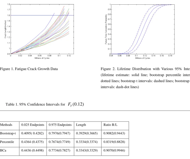
. 5 NUMERICAL EXAMPLESThe fatigue crack growth data from Hudak, Saxena et al. [4] is utilised to demonstrate bootstrap methods. The same data are also used by Lu and Meeker [12] to fit a general path degradation model. There are 21 test units, each giving a sample path. All the units have an initial crack length of 0.9 inches. In Lu and Meeker [12], failure is defined when the crack growth passes 1.6 inches. In this paper, the same definition is also adopted. The 21 sample paths are illustrated in Figure 1.
Three bootstrap methods are used respectively to estimate the confidence interval for lifetime distribution when modelling these degradation paths with the basic Gamma model. The results are shown in Figure 2.
As shown in Figure 2, the intervals obtained by bootstrap percentile are almost the same as the bootstrap BCa intervals, but are narrower than those of bootstrap-t. This relationship is consistent for all the t.
At the censoring time, i.e. t=0.12, the lifetime cumulative probability confidence intervals by different methods are listed in Table 1. The estimate of cumulative probability is 0.6167. The interval length is calculated as the difference between the upper endpoint and the lower endpoint. The right to left ratio is defined as the ratio of distances from the upper and lower endpoints to the estimate.
Figure 1. Fatigue Crack Growth Data Figure 2. Lifetime Distribution with Various 95% Intervals (lifetime estimate: solid line; bootstrap percentile intervals: dotted lines; bootstrap t intervals: dashed lines; bootstrap BCa intervals: dash-dot lines)
Table 1. 95% Confidence Intervals for
F
T(
0
.
12
)
Methods 0.025 Endpoints 0.975 Endpoints Length Ratio R/L
Bootstrap-t 0.4095( 0.4282) 0.7976(0.7947) 0.3929(0.3665) 0.9082(0.9443)
Percentile 0.4364 (0.4375) 0.7674(0.7749) 0.3334(0.3374) 0.8319(0.8828)
BCa 0.4436 (0.4498) 0.7734(0.7827) 0.3343(0.3329) 0.9070(0.9946)
The bootstrap calibration is utilized to examine the coverage accuracy of confidence intervals obtained by these three bootstrap methods. An interval is said to be accurate if the coverage probability of endpoints equal to the desired level, i.e.
v
(
u
)
=
u
. The relationship of the actual coverage and the nominal coverage could be demonstrated explicitly by plotting one against the other.v
>
u
indicates that the estimated intervals are wider than the real intervals, and vice versa. We plotv
against
u
in Figure 3 for lifetime cumulative probability atT
=
0
.
12
. The calibrated values are shown in parentheses in Table 1. The bootstrap calibration makes the bootstrap-t interval shorter but has few effects on the confidence intervals by bootstrap percentile and BCa methods. In terms of the interval symmetry improvement, the bootstrap calibration performs well for all three intervals.Figure 3. Estimated Calibration Curves for Three Bootstrap Methods (From left to right: bootstrap-t, percentile, and BCa respectively. The dashed line represents the diagonal line)
From Figure 3 it can be seen that for the basic Gamma degradation process, the bootstrap-t methods generally produce confidence intervals having coverage probability larger than the nominal value. In other words, the bootstrap-t methods are conservative here. On the contrary, the coverage probability of the confidence interval calculated by BCa is slightly smaller than the desired level, i.e. the BCa method is anti-conservative in this application. We find the percentile method generates almost exact confidence intervals in this case.
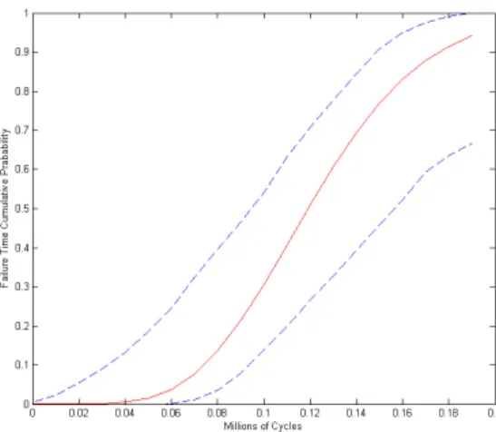
Lawless [1] proves that there are random effects existing in the crack growth data which is being used here. Therefore, it is also valid to fit the random effects Gamma process to this data. Figure 4 and Figure 5 show the lifetime distribution and three bootstrap confidence intervals when treating the deterioration as a process with random effects rather than a basic Gamma process.
As can be seen from Figure 4, unlike in the case of the basic Gamma process, confidence interval endpoints of bootstrap percentile here are not consistently smaller than those of bootstrap BCa. At the early stage of crack growth, the BCa endpoints are larger than those of percentile, while at the late period the percentile endpoints are larger than the BCa’s.
The bootstrap-t intervals tend to be unstable and have wider confidence intervals than both percentile and BCa intervals, which can be seen clearly from Figure 4 and Figure 5. But it is still worthwhile to analyse and compare its intervals with those of others.
Figure 4. 95% Confidence Intervals through Bootstrap Percentile and BCa (lifetime estimate: the solid line; bootstrap percentile intervals: dotted lines; bootstrap BCa intervals: dash-dot lines)
Figure 5. 95% Confidence Intervals through Bootstrap-t (lifetime distribution estimate: the solid line; bootstrap-t confidence intervals: dashed line)
The relationship between
v
andu
is plotted in Figure 6. The dotted, dash-dot and solid curves correspond to t=0.16, 0.12 and 0.08 respectively. As the time increases, bootstrap-t confidence intervals’ coverage probability varies around the nominal value while intervals by the percentile method changes from anti-conservative to conservative. For the BCa method, results are more stable. The actual coverage probability converges to the nominal value but generally these curves are still under the diagonal line, which means the confidence intervals obtained by the BCa are anti-conservative here.Figure 6. Estimated Calibration Curves When Considering Random Effects (From left to right: bootstrap-t, percentile, and BCa; the dashed line represents the diagonal line)
6 CONCLUSION
In this paper, three bootstrap methods have been applied to build confidence intervals for the lifetime distribution calculated by Gamma degradation models. The bootstrap calibration is conducted to assess the coverage probability of the estimated confidence intervals. The calibration shows that for different Gamma processes, these three bootstrap confidence interval generation methods have different coverage accuracy. For the basic Gamma process, the bootstrap percentile produces the best results while the bootstrap-t methods are conservative and BCa is slightly anti-conservative. For the Gamma process considering random effects, the three methods result in quite different outcomes. The BCa intervals are generally anti-conservative and have coverage probability closer to the nominal value while the other two confidence intervals vary around the nominal value. The BCa method produces reasonable results for both basic and random effect Gamma models in the case study. It can be concluded that the BCa method is recommended for generating confidence intervals in this Gamma degradation analysis.
REFERENCE
1 Lawless J & Crowder M. (2004) Covariates and Random Effects in a Gamma Process Model with Application to Degradation and Failure. Lifetime Data Analysis, 10(3), 213-227.
2 Doganaksoy N. (1995) Likelihood Ratio Confidence Intervals in Life-data Analysis. Balakrishnan N (Ed.). Recent Advances in Life Testing and reliability. pp. 359-376.
3 DiCiccio TJ & Efron B. (1996) Bootstrap Confidence Intervals. Statistical Science, 11(3), 189-228.
4 Hudak SJ, Saxena A, Bucci RJ & Malcolm RC. (1978) Development of Standard Methods of Testing and Analyzing Fatigue Crack Growth Rate Data, Technical Report AFML-TR-78-40, Westinghouse R&D Center, Westinghouse Electric Corporation. Pittsburgh, PA, 1978.
5 van Noortwijk JM. A Survey of the Application of Gamma Processes in Maintenance. Reliability Engineering & System Safety, In Press, Corrected Proof.
6 Jeng SL & Meeker WQ. (2000) Comparisons of Approximate Confidence Interval Procedures for Type I Censored Data. Technometrics, 42(2), 135-148.
Applied Mathematics, Philadelphia. Society for Industrial and Applied Mathematics(SIAM).
8 Efron B & Tibshirani R. (1986) Bootstrap Methods for Standard Errors, Confidence Intervals, and Other Measures of Statistical Accuracy. Statistical Science, 1(1), 54-77.
9 Efron B & Tibshirani R. (1993) An Introduction to the Bootstrap. New York, NY: Chapman & Hall.
10 Loh WY. (1987) Calibrating Confidence Coefficients. Journal of the American Statistical Association, 82(397), 155-162. 11 Efron B. (1987) Better Bootstrap Confidence Intervals. Statistical Science, 82(397), 171-185.
12 Lu CJ & Meeker WQ. (1993) Using Degradation Measures to Estimate a Time-to-failure Distribution. Technometrics, 35(2), 161-174.
ACKNOWLEDGEMENT
The authors gratefully acknowledge the financial support provided by the QUT Faculty of Built Environment & Engineering and the Cooperative Research Centre for Integrated Engineering Asset Management (CIEAM).