Dynamic Switching State Systems for Visual Tracking

(1)

Dynamic Switching State Systems

for Visual Tracking

zur Erlangung des akademischen Grades eines

Doktors der Ingenieurwissenschaften

von der KIT-Fakultät für Informatik des Karlsruher Instituts für Technologie (KIT)

genehmigte

Dissertation

von

Stefan Becker

aus Lebach

Tag der mündlichen Prüfung: 24.04.2020

Erster Gutachter: Prof. Dr.-Ing. Jürgen Beyerer

(2)

(3)

Abstract

Estimating the motion state of objects is a central component of most visual tracking pipelines. Therefore, object observations provided by an appearance model, representing the object in image space, serve as input for the actual filtering and the prediction into future frames. Under real-life conditions, the dynamics of tracked objects are subject to change over time. Especially in such maneuver scenarios, current methods struggle to deal with the model mismatch due to varying system characteristics.

This thesis addresses the problem of how to capture the dynamics of maneu-vering objects in an efficient and reactive way. Towards this end, the per-spective of recursive Bayesian filters and the perper-spective of deep learning ap-proaches on state estimation are considered and their functional viewpoints are brought together.

The starting point of this thesis is theinteracting multiple-model(IMM) filter, as the most common representative Bayesian formulation for dealing with model mismatches or rather maneuvering objects. For a model mismatch scenario, in which tracking is done directly in image space, a state de-coupling and a re-coupling scheme are introduced as modifications for an improved design compared to the standard IMM filter.

In order to deal with two maneuver types, switching noise levels and switch-ing dynamics,recurrent neural network(RNN)-based approaches are pro-posed as alternatives to IMM filtering. The approaches maintain the func-tionality of an IMM filter while reducing the amount of required filter tuning. With a focus on applications in the surveillance and intelligent vehicle do-mains, the effectiveness of RNN-based solutions is demonstrated for the ex-emplary tasks ofpath predictionandintention prediction, reflecting the most

(4)

common prototypical maneuver types. The presented RNN-based network yields performance comparable to other existing relevant methods on a pub-lic benchmark. The suggested modifications help to achieve a robust predic-tion performance with regard to switching noise levels. For sudden mopredic-tion changes, a proposed RNN-based IMM surrogate can capture the change in the dynamical behavior mare reliably than the Bayesian filter counterparts. The abilities of the RNN-IMM are evaluated in extensive experiments on real-world and synthetic datasets, reflecting prototypical maneuver situations of pedestrians in the application domain of intelligent vehicles.

(5)

Kurzfassung

Die Schätzung des Bewegungszustands von Objekten ist eine zentrale Komponente für die video-basierte Objektverfolgung. Dabei werden Objekt-beobachtungen, die von einem Erscheinungsmodell geliefert werden und das Objekt im Bildraum repräsentieren, als Eingabe für die Filterung und die Vorhersage in zukünftige Frames verwendet. Unter realen Bedingungen variiert die Dynamik des verfolgten Objektes über die Zeit. Besonders in solchen Manöversituationen haben aktuelle Methoden wegen Modellfehlan-passungen aufgrund der variierenden Systemeigenschaften Schwierigkeiten den Bewegungszustand des Objektes zu schätzen.

Diese Arbeit befasst sich mit dem Problem der effizienten und reaktiven Er-fassung der Dynamik von manövrierenden Objekten. Zu diesem Zweck wer-den die Perspektive rekursiver Bayes’scher Filter und die Perspektive tiefer lernender Ansätze zur Zustandsschätzung betrachtet und ihre funktionalen Sichtweisen zusammengeführt.

Ausgangspunkt dieser Arbeit ist das interacting multiple-model (IMM)-Filter, als einer der am häufigsten verwendete Ansätze basierend auf einer Bayes’sche Formulierung zum Umgang mit Modellfehlanpassungen bzw. ma-növrierenden Objekten. Für ein Modellfehlanpassungsszenario, bei dem die Objektverfolgung direkt im Bildraum erfolgt, werden eine Zustandsentkopp-lung und ein RückkoppZustandsentkopp-lungsschema als Modifikationen für ein verbesser-tes Design im Vergleich zum Standard-IMM-Filter eingeführt. Zum besseren Umgang mit den zwei Manövertypen von variierenden Rauschpegeln und

(6)

variierenden Objektdynamiken werdenrecurrent neural network (RNN)-basierte Ansätze als Alternative zum IMM-Filter vorgestellt. Die Ansätze bil-den die Funktionalität eines IMM-Filters ab und reduzieren gleichzeitig bil-den Umfang der erforderlichen Filterabstimmung.

Mit dem Schwerpunkt auf Anwendungen in den Bereichen Videoüberwa-chung und intelligente Fahrzeuge wird die Wirksamkeit der vorgestellten RNN-basierten Ansätze exemplarisch für Aufgabenstellungen der Pfad-vorhersage und der Intentionsvorhersage demonstriert. Die ausgewählten Anwendungen spiegeln prototypische Manöversituationen wieder. Ein vor-gestelltes RNN-basiertes Netzwerk erzielt eine Leistung vergleichbar mit relevanten Methoden auf dem aktuellen Stand der Technik auf einem öf-fentlichen Benchmark. Die vorgeschlagenen Modifikationen tragen dazu bei eine robuste Vorhersageleistung in Bezug auf die Rauschpegel zu er-reichen. Bei plötzlichen Bewegungsänderungen kann ein vorgeschlagenes RNN-basiertes IMM-Surrogat die Änderung im dynamischen Verhalten zu-verlässiger erfassen als die Bayes’sche Filter Pendants. Die Fähigkeiten des RNN-IMM werden in umfangreichen Experimenten auf realen und syntheti-schen Datensätzen, die prototypische Manöversituationen von Fußgängern im Anwendungsbereich intelligenter Fahrzeuge widerspiegeln, evaluiert.

(7)

Acknowledgements

This thesis is the result of my work in the departmentObject Recognitionat the Fraunhofer Institute of Optronics, System Technologies and Image Exploitation IOSB. I was in the fortunate position of receiving much individual support in a variety of ways.

First of all, I would like to thank my advisor Prof. Dr.-Ing. Jürgen Beyerer for his guidance and feedback, which were invaluable to complete this thesis. I am grateful to Prof. Ph.D. Brendan T. Morris, Prof. Dr. Bernhard Beckert, Prof. Ph.D. Mehdi B. Tahoori, and Prof. Dr. Peter Sanders for agreeing to be part of my examination committee. In particular, I would like to thank Ph.D. Brendan T. Morris for his interest in my work and for being in the committee as a second advisor.

Special thanks go to my supervisors Dr. Wolfgang Hübner and Dr. Michael Arens atFraunhofer IOSBfor providing conditions, feedback, and freedom to prepare this thesis.

I want to acknowledge my colleagues of the departmentObject Recognitionfor their constant assistance and in particular, my colleagues of theVideo Content Analysisgroup. The support and the conversations were essential for solving various technical challenges.

Lastly, I want to thank my family and friends for their advice and their en-couragement throughout all phases of this work.

(8)

(9)

Notation

This chapter introduces the notation and symbols which are used in this thesis.

General notation

Scalars italic Roman and Greek lowercase letters 𝑥, 𝛼

Sets calligraphic Roman uppercase letters 𝒟

Vectors bold Roman lowercase letters 𝐭

Matrices bold Roman uppercase letters 𝐑

State spaces bold calligraphic Roman uppercase letters 𝓧

In multidimensional sets of elements related to time series, the first super-script index denotes time.

Distributions

𝒩 Gaussian distribution

(12)

Numbers, indexing and conventions

ℕ natural numbers

ℝ real numbers

𝑘, 𝑡 discrete points in time

𝑖, 𝑗, ℓ, 𝑞 indexing for objects, observations and points

⌈⋅⌉ ceil operator, the least integer greater than or equal to the value.

State modeling and probabilities

𝓧 (dynamical) state-space 𝓗 (recurrent) state-space 𝓩 observation space 𝓨 target space 𝑓(⋅) dynamical model ℎ(⋅)𝑜𝑏𝑠 observation model

𝐅 system matrix of the Kalman Filter

𝐆 noise gain matrix of the Kalman Filter

𝐇 observation matrix of the Kalman Filter

𝐊 Kalman gain

𝔼[⋅] expectation value

(13)

𝐡𝑘 _{(recurrent) state vector at time}_𝑘

𝐳𝑘 _{observation vector at time}_𝑘

𝐲𝑘 _{target vector at time}_𝑘

𝑚𝑘 _{dynamical mode at time}_𝑘

𝐯𝑘 _{process noise at time}_𝑘

𝐰𝑘 _{observation noise at time}_𝑘

𝐐𝑘 _{process noise covariance matrix at time}_𝑘

𝐑𝑘 _{observation noise covariance matrix at time}_𝑘

𝐏 covariance matrix

𝐏𝑘

𝐱𝐱 (dynamical) state covariance matrix

𝐏𝑘

𝐳𝐳 observation covariance matrix

𝐏𝐱𝐱𝑘,− prior probability

𝐏𝐱𝐱𝑘,+ posterior probability

𝑝(𝐱𝑘₎ _{probability density function (pdf)}

𝑃(𝑚𝑘₎ _{probability mass function (pmf)}

𝑝(𝐱𝑘+1_|𝐱𝑘_,...) _{transition density}

(14)

(15)

1

Introduction

One fundamental ability essential for intelligent autonomous systems to see, understand, and react to the environment is to track objects of interest in im-age sequences. Its applications cover a broad range from intelligent vehicles to robot navigation and smart video surveillance. For example, the ability to anticipate the actions of pedestrians in a scene and to predict their future po-sitions is a safety issue for autonomous vehicles and other vision-based active safety systems.

?

Figure 1.1:Scenes captured from an approaching vehicle, the most important question being whetherthe pedestrian is going to cross the street. Traditionally, such questions are tackled with adaptive recursive Bayesian filters [Sch13].

Despite enormous advances in extracting observations of objects from im-ages due to deep learning, the actual filtering and the prediction into future frames are mainly restricted to the application of recursive Bayesian filters. The problem-specific choice of their design parameters, such as connecting

(16)

the object motion uncertainty and its predictability to physical system pa-rameters or the observation uncertainty, requires not only well-suited phys-ical models, but also a large amount of engineering. Especially in situations where the tracked objects perform a maneuver, this has proved a challenging task. A maneuver is any motion characteristic that an object is performing other than the dynamical model used by the filter. An illustrative example for a variation in the dynamics, which poses significant challenges for the filters to adapt, is to determine if a pedestrian is going to cross the street (see fig-ure1.1). Such situations additionally require the choice of various adequate dynamical models, including associated transition modeling.

Towards this end, the overarching research question of this thesis is how to capture the dynamics of maneuvering objects in image sequences effectively. Maneuvering objects can be defined by either being subject to random per-turbations i.e., different noise levels or subject to sudden motion changes. The dynamical model acts as one component of a larger vision system whose tasks mainly consist of providing additional information for further process-ing steps, supportprocess-ing appearance models by bridgprocess-ing detection failures, and forecasting the behavior by predicting future states.

1.1 Problem Statement

Given a short sequence of observations𝒵generated by an appearance model of a visual tracker, we are interested in estimating the state of a maneuver-ing object. In the followmaneuver-ing, systems where the discrete-time version of the motion or dynamical model can be formalized as follows are considered:

𝒴 = 𝑓𝜃(𝒵0∶𝑘,𝒞0∶𝑘) + 𝝐, (1.1)

The aim is to estimate the expected conditioned states of the object

(17)

Here, 𝒴 describes the states or state distributions of a tracked object, 𝒞

describes additional contextual cues extracted from the observed image sequences and 𝝐describes an additional error term. In Bayesian filtering, models of this type are called state-space models or dynamical systems, whereas in deep learning, they are referred to as recurrent neural networks. This thesis includes discussions on both formulations and their connection by maximum likelihood inference. In order to effectively capture the dy-namics of maneuvering objects and to reduce the amount of engineering, a comparable deep learning solution to adaptive recursive Bayesian filtering is introduced. The research questions in this context are answered along with the prototypical types of maneuvers, abrupt change of motions and random perturbations. The main application areas throughout this thesis are intelligent vehicles and automated surveillance systems.

1.2 Contributions

The starting point of this thesis are adaptive filters and their most common representative, theinteracting multiple-model(IMM) filter [Blo88]. Based on a Bayesian formulation, the IMM filter is designed for capturing motion uncertainties and modeling complex object dynamics in situations where the object undergoes sudden changes. The IMM filter can be used to combine sev-eral dynamical models and offers a good compromise between performance and complexity. This thesis contributes to an improved design of a basic IMM filter as a module in a visual tracking pipeline by introducing both a state de-coupling and a re-coupling scheme as modifications:

• Firstly, when relying solely on visual cues, the benefit of a suggested de-coupling of the state estimate of an IMM filter is demonstrated [Bec16].

• Secondly, a state re-coupling scheme is introduced which helps to better deal with the corresponding observation uncertainties of such a tracking pipeline [Bec18a].

(18)

Although the IMM filter has some drawbacks, it is still a core element for many state-of-the-art applications. In order to reduce the amount of required engi-neering and to learn an improved dynamical model structure, a contribution of this thesis is the transfer of the IMM functionality into a comparable deep learning architecture. Since adaptive filters and in particular the IMM filter are designed to deal with maneuvering objects, in the following two major maneuver types are considered separately:

• Switching noise levels: The effectiveness of deep neural networks for predicting future pedestrian states is evaluated. A proposed network achieves state-of-the-art performance on publicly available datasets [Bec18c]. The results can be accessed on theTrajNetwebsite

(http://trajnet.stanford.edu/, last accessed 19.12.2019). The ranking of different predictors combines the final displacement error and the average displacement error for predicting the next12states of pedestrian trajectories pooled over the datasets. The proposed network is an RNN-encoder with a dense layer on top for projecting into the observation space. Although being simple at core, the network can achieve a performance comparable to more elaborated models in terms of considering more cues than solely position information.

• Switching behavior: The connections to the IMM filter are explored and an IMM filter surrogate is presented (RNN-IMM). Similar to an IMM filter solution, the presented RNN-IMM assigns a probability value to different dynamical modes and, based on them, generates a multi-modal distribution over future object states as output[Bec19b, Bec19a]. The switching behavior is thoroughly analyzed for prototypical, critical maneuver situations, such as abending in maneuver of pedestrians. The presented RNN-IMM solution reduces not only the amount of explicit modeling of filter parameters but enables an improved maneuver onset and maneuver termination behavior.

In order to provide a learned reference trajectory for pooled object trajectory data, this thesis contributes by introducing an alignment network.

(19)

• Alignment network: The application of hard-coded normalization strategies on pooled trajectories shifts the variation along the trajectory. Hence, the arbitrarily chosen references hinder applying clustering approaches. The proposed network learns a freely adjustable prototype as a reference trajectory. Firstly, the resulting prototype reflects the minimum variance of the input trajectories, which allows deducing the dominating dynamical behavior. Secondly, with a fixed reference, the conditions for clustering approaches and out-of-distribution detections are improved.

Overall, this thesis is motivated by uniting the interconnected Bayesian and deep learning perspectives on maneuver prediction. In response to the re-search question on how to effectively capture changing object dynamics in image sequences, a transfer to an IMM filter comparable neural networks is introduced.

1.3 Outline

The thesis is structured as follows: Chapter2introduces the theoretical back-ground in order to unite the functional views of deep learning and Bayesian filtering on object tracking. Furthermore, current state-of-the-art is surveyed for selected exemplary applications. In chapter3, the problem of maneuvering object tracking is considered from the Bayesian filtering perspective, result-ing in improved IMM filter designs. Chapter4presents an alternative deep learning-based solution in order to reduce the amount of hand-tuning of the filters and to provide an effective solution for the switching state problem. Conclusions are drawn in chapter5.

(20)

(21)

2

Perspectives on State Estimation

from Visual Observations

In this chapter, the perspectives of deep learning and recursive Bayesian fil-tering on (visual) object tracking are united. Based on the united functional view, the contributions of this thesis are positioned with respect to existing literature and to specific applications.

2.1 What is Visual Tracking?

Vision-based or visual tracking is defined as the process of using image obser-vations and a predictive dynamical model to consistently estimate the state(s) of one or more object(s) over the discrete-time steps corresponding to video frames [Mag11]. Thereby recursive Bayesian filtering acts mostly as a top-down process for state estimation, which involves incorporating prior infor-mation about the scene or object to connect the object dynamics to physical systems [Bla03]. This tracking pipeline with top-down filtering is often re-ferred to as detection-by-tracking [And08] and without top-down filtering as tracking-by-detection. A block diagram for a single object visual tracking pipeline is visualized in figure2.1.

Vision-based tracking of a single object is formulated as the estimation of a time series𝒵 = {𝐳𝑘_{∶ 𝑘 ∈ ℕ}}_{over a set of discrete-time instances}_𝑘_{, based on}

the informationℐ = {𝐈𝑘 _{∶ 𝑘 ∈ ℕ}}_{from the set of images. The vector-valued}

time series𝒵is considered as the states of the object and is mainly referred to as the trajectory of the object. However, for recursive Bayesian filters or

(22)

Object initialization

Appearance model Visual

representation Statisticallearning estimationState Localization

Figure 2.1:Block diagram of a visual tracking pipeline which shows the main components of a tracking cycle.

dynamical systems ¹ the term state𝒳 = {𝐱𝑘 _{∶ 𝑘 ∈ ℕ}}_{refers to a collection of}

variables such as position, velocity, orientation, which are indirectly observed through noisy observations.

Since the focus of this thesis is neither on building an appearance model for object detection nor the necessary feature extraction, but on the top-down state estimation, it is crucial to distinguish between the term states clearly. The term observation𝐳𝑘 _{will be used to describe the object representation}

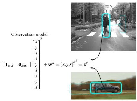
(e.g., bounding box, centroid, blobs) in the image generated by an appearance model of a detector or a visual tracker. Thus, appearance modeling basically boils down to representing object pixel intensities. The resulting associated image region is the observation serving as input for the dynamical state esti-mation. Pedestrian detections in the form of enclosing bounding-boxes is an illustrative example of an observation space𝓩. Observation, detection, and object state interchangeably refer to the shape approximation in the image in contrast to the dynamical state𝐱𝑘_{, which fully describes a dynamical system.}

In figure2.2, commonly used object representations for describing the location and an approximation of the object shape are depicted. For the goal of tracking an object in the2D image space, the minimal form of𝐳𝑘_{is the center position}

of the object in𝐈𝑘_.

¹ The terms state-space models and dynamical systems are used interchangeably in this thesis. Whereas the term state-space models originates from probabilistic modeling, the term dynam-ical systems originates from signal processing. Bayesian filtering refers to the Bayesian way of formulating optimal filtering for dynamical systems.

(23)

Figure 2.2:Examples of object states for different visual tracking tasks.

Deep-tracking based approaches are mostly tailored to image processing tasks such as classification and detection, thus detection-by-tracking with a Bayes-ian filter is still very common [Kre17]. The tasks of the Bayesian filter within the overall pipeline are:

• The support of the appearance model to bridge detection failures or occlusion situations.

• Provide additional information for subsequent processing stages.

• Enhance the detection robustness.

• Estimate indirectly observables.

• Forecast the behavior of the object.

Within the pipeline, the tasks of the Bayesian filter can be explicitly associated with different types of inference problems: prediction, filtering, and smooth-ing. Because inference is a very general problem for machine learning models, the consideration of the filter functionality as an inference problem helps to unite the functional viewpoints. Furthermore, the types of required compu-tations are neatly separated in order to reason from sequential data correctly [Moh15].

(24)

2.2 One Problem - Two Functional Views

Recursive Bayesian filtering refers to the Bayesian way of formulating the es-timation of the hidden (dynamical) states using probability theory. Hence, the hidden dynamical states and the observations are assumed to be random vari-ables. The dynamical state itself is represented by means of aprobability density function(pdf)¹𝑝(𝐱𝑘₎ _{at time step}_𝑘_{. It is assumed that the} tran-sition density²𝑝(𝐱𝑘+1_|𝐱𝑘₎ _{is the same for all time instances and behaves}

according to a known system transition function. This function is referred to as the dynamical model (see equation1.1). Other commonly used terms include, among others, motion model, process model, and plant model. For recursive Bayesian filtering, the dynamical model can be written as

𝐱𝑘+1_{= 𝑓}𝑘_(𝐱𝑘_{, 𝐯}𝑘₎_. _(2.1)

Here,𝑓𝑘_(⋅)_{is a non-linear function and}_𝐯𝑘_{the process noise. In the remainder}

of this thesis, only discrete-time models are considered because the observa-tions are a set of discrete-time instants. The time steps are related through

𝑡𝑘+1 _{= 𝑡}𝑘_{+ Δ𝑇}_{, where}_Δ𝑇_{is the sampling time. The dynamical state}_𝐱_is

assumed to be an unobserved Markov process, and𝐳are the observations of

ahidden Markov model(HMM). The observation or measurement model

maps the hidden dynamical state into the observation space and is given by

𝐳𝑘 _{= ℎ}𝑘

𝑜𝑏𝑠(𝐱𝑘, 𝐰𝑘), (2.2)

with the non-linear observation functionℎ𝑘𝑜𝑏𝑠(⋅)and observation noise𝐰𝑘.

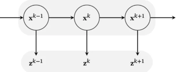
A graphical model, which expresses the conditional dependence structure of such an HMM, is depicted in figure2.3(see for example [Kol09]). The structure of the model complies with a directed acyclic graph representing the factor-ization of the joint probability.

¹ In case of a discrete state-spaceprobability mass function(pmf)𝑃(𝐱𝑘₎_.

(25)

𝐱𝑘−1 _𝐱𝑘 _𝐱𝑘+1

𝐳𝑘−1 _𝐳𝑘 _𝐳𝑘+1

Figure 2.3:A graphical model specifying the conditional relations for a dynamical system. As aforementioned, the conditional density𝑝(𝐱𝑘+1_|𝐱𝑘₎_{, which depends on}

the dynamical model, is assumed to be stationary. This is equivalent to as-suming that the parameters of the transition function are shared across time steps [Moh15]. Thus, it is possible to directly connect torecurrent neural networks(RNNs) [Goo16,Rum88] and the loss function of RNNs using maxi-mum likelihood estimation. Under the Markov assumption, the probability of an observed sequence𝒵according to adynamical system(DS) as depicted in figure2.3can be calculated by marginalizing over𝐱𝑘_:

𝑝(𝐳0_{, … ,𝐳}𝐾_{) =} _∏ 𝑘

∫ 𝑝(𝐳𝑘_,𝐱𝑘₎_d_𝐱𝑘_with _(2.3)

𝑝(𝐳𝑘_,𝐱𝑘_{) =} _𝑝(𝐳𝑘_|𝐱𝑘_)𝑝(𝐱𝑘_|𝐱𝑘−1₎

Using the negative log-likelihood, the following loss function can be obtained:

ℒ(Θ)𝐷𝑆 = − ∑ 𝑘

log∫ 𝑝(𝐱𝑘_|𝐱𝑘−1_)𝑝(𝐳𝑘_|𝐱𝑘₎_d_𝐱𝑘 _(2.4)

For deterministic transition dynamics,

(26)

the loss function can be reformulated to ℒ(Θ)𝐷𝑆 = − ∑ 𝑘 log𝑝(𝐳𝑘_|𝑓 Θ(𝐱𝑘−1,𝐳𝑘−1)) (2.6) = − ∑ 𝑘 log𝑝(𝐳𝑘_|𝑓 Θ(𝐱𝑘−1)).

Next, the loss function is recovered from the perspective of RNNs. According to equation2.4, the goal is to capture the probability of the observed sequence

𝒵. RNNs are extensions of multi-layer feed-forward networks, where hidden unitsℋ = {𝐡𝑘 _{∶ 𝑘 ∈ ℕ}}_{are used to encode an internal hidden state space}

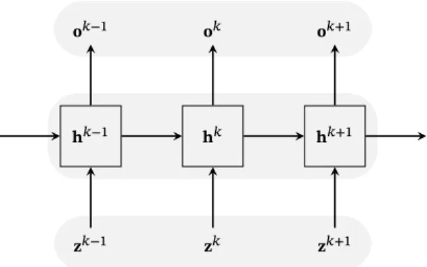
[Goo16]. In extension to multi-layer networks, the parameters are shared across different parts of a model. Here, the parameter of the transition func-tion are shared across time steps, resulting in a neural network where the activation of the hidden layers are fed back into the network along with the input. Figure2.4depicts the unfolded computational graph of an RNN, where the hidden state sequence is used to compute the output vector sequence

𝒪 = {𝐨𝑘 _{∶ 𝑘 ∈ ℕ}}_.

𝐡𝑘−1 _𝐡𝑘 _𝐡𝑘+1

𝐳𝑘−1 _𝐳𝑘 _𝐳𝑘+1

𝐨𝑘−1 _𝐨𝑘 _𝐨𝑘+1

Figure 2.4:Recurrent neural network seen as an unfolded computational graph. Each node is associated with a particular time instance.

(27)

The unfolded model structure corresponds, similarly to recursive Bayesian fil-tering, to a directed acyclic computational graph. Thus, the recurrent network processes information by incorporating it into the state𝐡that is passed for-ward through time by the transition function. The hidden state for one time step is given by

𝐡𝑘+1_{= 𝑓}

Θ(𝐡𝑘, 𝐳𝑘+1). (2.7)

For a basic RNN [Elm90] the transition function is given by

𝐡𝑘+1_{= 𝜙 (𝐖}

ℎℎ𝐡𝑘+ 𝐖ℎ𝑧𝐳𝑘+1+ 𝐛ℎ), (2.8)

where𝐖ℎℎand𝐖ℎ𝑧represents the weights,𝐛ℎthe biases of a recurrent layer,

and𝜙(.)an activation function. Based on ideas of graph unrolling and para-meter sharing, a wide variety of recurrent neural networks can be designed [Goo16]. For the moment, we stick with an RNN as depicted in figure2.4that generates an output at each time step and uses a hidden-to-hidden recurrent connection as described above. The depicted RNN does not specify what form the output and loss function take. Thus, the output𝐨𝑘_{can be used to}

param-eterize a predictive distribution𝑝(𝐳𝑘+1_|𝐨𝑘₎_{over possible next observations}

𝐳𝑘+1_{. In order to match}_𝐳_{, the form of}_𝑝(𝐳𝑘+1_|𝐨𝑘₎_{must be chosen carefully.}

The problem of finding a good predictive distribution can be very challenging and is usually referred to as probability density modeling [Gra13a]. Given a hidden state, the output is computed as follows

𝐨𝑘 _{= 𝑜 (𝐖}

ℎ𝑜𝐡𝑘+ 𝐛𝑜), (2.9)

where𝑜 (⋅)is the output layer function,𝐖ℎ𝑜denotes a weight matrix and𝐛𝑜

denotes a bias vector. The complete network defines a function, parameter-ized by the weight matrices, from observations𝐳0∶𝑘_{to the output vector}_𝐨𝑘_.

Equation2.7can be considered as the RNN equivalent of the dynamical model, and equation2.9can be considered as the RNN equivalent of the observation model. The probability of an observed sequence𝒵as estimated by an RNN is

(28)

given by

𝑝(𝐳0_{, … ,𝐳}𝐾_{) = ∏} 𝑘

𝑝(𝐳𝑘+1_|𝐨𝑘₎_. _(2.10)

The corresponding loss function of an RNNs using maximum likelihood esti-mation can be defined as:

ℒ(Θ)𝑅𝑁𝑁 = − ∑ 𝑘 log𝑝(𝐳𝑘+1_|𝐨𝑘₎_{, or rather} _(2.11) = − ∑ 𝑘 log𝑝(𝐳𝑘+1_|𝑓 Θ(𝐡𝑘−1, 𝐳𝑘)). (2.12)

Due to the deterministic nature of RNNs, the computation of the predictive distributions is realized by the feed-forward operations in the unfolded net-work. By applyingbackpropagation through time(BPTT) [Wil95] to the computational graph, the partial derivatives of the loss with respect to the network weights can efficiently be calculated, and the network can be trained using stochastic gradient descent.

When comparing the loss functions of equation2.12and2.6, it becomes evi-dent that the RNN loss corresponds to maximum likelihood estimation with deterministic dynamics. According to Bayesian filtering, the result for the associated inference problems are given in form of a conditional probability density that represents the dynamical state estimate [Hub15]. The estima-tion tasks depend on the relaestima-tion between the time steps𝑘and𝐾. If𝑘 < 𝐾, the estimation problem is referred to asprediction(inferring the future), for

𝑘 = 𝐾the estimation is referred to asfiltering,update, orcorrection respec-tively (inferring the present), and if𝑘 > 𝐾, it is referred to assmoothing (infer-ring the past). Prediction and filte(infer-ring are typically performed on-line, while smoothing is an off-line estimation task, as it improves past state estimates given additional information. For Bayesian filters, the conditional densities are calculated recursively under the assumption that the dynamical state is a Markov process. For the tracking pipeline described in section2.1and for

(29)

many other practical applications, prediction and filtering are performed al-ternatingly, which is commonly referred to asprediction-updatecycle. Based on the above drawn connections between the Bayesian perspective and the RNN perspective, for both on-line estimation tasks of recursive Bayesian fil-ters, there exists an RNN counterpart, wherepredictionandupdateare realized by feed-forward operations in the unfolded network. For applying Bayesian filtering, strict assumptions such as Gaussian transitions are required to solve the inference problem, but those assumptions are commonly violated in a real environment. Before the seminal Kalman filter [Kal60] is introduced as a basic dynamical state estimator, this thesis is positioned with respect to the existing literature for two selected tasks, where the role of a top-down state estimator as part of a vision-based tracking is a crucial component. While extracting the observation from images is specific to computer vision, inference is very general, and the field of machine learning and pattern recognition is entered. In order to narrow down the large number of existing approaches originating from different communities, these approaches are categorized with respect to the applied motion model, the level of contextual information used, and the time horizon under consideration. The following discussion uses mainly the Bayesian perspective for positioning the contributions compared to related work.

2.3 Related Work

The two selected tasks, in which higher-level processing strongly relies on the state estimator, arepath predictionandintention prediction. Wherebypath pre-dictionis mainly tackled as a purepredictionproblem forintention prediction, bothpredictionandfilteringis mostly done jointly (see for example [Gav99]).

2.3.1 Path Prediction

In tasks such aspath prediction, the termagent often denotes the dynamic objects of interest such as robots, pedestrians, cyclists, cars, or other human-driven vehicles. The target agent is the dynamic object for which the motion

(30)

Motion prediction Modeling Physics-based Single-model methods Multiple-model methods Pattern-based Non-sequential models Sequential models Planning-based Forward planning methods Inverse planning methods Contextual cues Static enviroment Unaware Obstacle-aware Map-aware Sematic-aware Dynamic enviroment

Unaware Indiviudal-_aware

Group-aware Target agent cues Motion state Articulated pose Semantic attributes

Figure 2.5:Overview of the taxonomy of categories according to Rudenko et al. [Rud19]. The categorization of this thesis within the taxonomy is highlighted in red.

prediction is done and corresponds to our tracked object. The termpathis here restrictively used for a sequence of positions, and the termtrajectorycan include additional information for describing the movement of the object. In

(31)

our case, the term trajectory corresponds to a sequence of object states (see section2.1) ¹ However, the focus here is onpath prediction, but the predic-tion of video frames, acpredic-tions, articulated mopredic-tion, or human activities often rely on the same motion prediction methods. As explained, there is a cross-disciplinary interest and a fast-growing body of work for motion prediction. In order to categorize the different prediction methods, we built on the tax-onomy introduced by Rudenko et al. [Rud19]. In accordance with this taxon-omy, motion prediction is categorized with respect to the modeling approach and the type of contextual cues. In figure2.5, the categories of the taxonomy introduced by Rudenko et al. are visualized.

Categorization from other related surveys may differ slightly, but are similar at their core. In order to name a few, there are surveys from application do-mains such as service robots [Kru13,Las17], intelligent vehicles [Ras19,Rid18, Bro16,Lef14], and computer vision [Hir18,Mur17,Mor08].

Most relevant for this thesis is the survey of Hirakawa et al. [Hir18]. They survey path prediction methods for vision-based systems, where all the consi-dered methods are realized on top of computer vision tasks, such as pedestrian detection. This corresponds precisely to our distinction between appearance modeling to generate observations as input data and the top-down state esti-mator. Hirakawa et al. categorize motion modeling approaches mainly into Bayesian models, energy minimization methods, deep learning methods, and inverse reinforcement learning methods. In addition, the approaches are cate-gorized depending on whether they explicitly use object features or environ-mental features extracted from a video. Rasouli and Kotsos [Ras19] survey pedestrian behavior in the application domain of intelligent vehicles and use the terms pedestrian factors and environmental factors to distinguish with re-spect to the awareness of a specific factor. With the taxonomy of Rudenko et al., this distinction is addressed by contextual cues. The categories utilized by Kruse et al. [Kru13], Lasota et al. [Las17] and Lefèvre et al. [Lef14] are also based on motion modeling and correspondingly included in the taxonomy.

¹ In robotics, the termpathis used for describing a space curve without a notion of time and the termtrajectoryis used for a path with a notion of time.

(32)

The taxonomy depicted in figure2.5enables to distinguish along the different modeling approaches and along an increasing level of contextual awareness. Using the motion modeling approach as a classification criterion, prediction approaches are divided inphysics-based methods,pattern-based methods and planning-based methods. The second criterion asks what contextual cues are exploited, leading to a classification betweentarget agentcues,dynamic envi-ronmentcues, andstatic environmentcues.

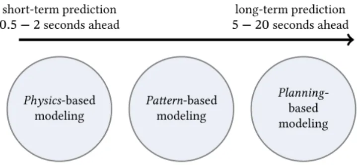
In addition to this taxonomy, we distinguish if some contextual cues are used in an additional processing step in order to associate the object’s dynamical state with the physical world. From the perspective of a Bayesian filter with a dynamical model, it is important if a reasonable observation model can be ap-plied. In particular,path prediction is mostly done on ground level, which implicitly requires additional assumptions about the environment or addi-tional sensors (LIDAR, stereo camera system) or approaches like structure-from-motion (SfM) [Sze10] to reconstruct a3𝐷scene. For example, an intelli-gent vehicle is accompanied by many additional sensors, which allow the ac-tual prediction of dynamic objects being done in an ego-motion compensated vehicle centered coordination system. Thus, even when the environmental cues are not used as input for the motion prediction itself, the overall vision-based system is aware of its environment. Thus, the system implicitly relies on more contextual cues. However, there exist several scenarios where this mapping is unknown, includes substantially higher expense, or is an overall unsolved problem. An example is general object tracking. In such a case, the object is directly tracked in image space on randomly selected videos. In several domains, this implicit knowledge of the environment is presumed but not always given. An example from the domain of visual surveillance is video recordings without extrinsic or intrinsic calibration of the cameras. The con-dition of being able to rely on mapping to the physical world or not is referred to as explicit or implicit contextual cues in the remainder of this thesis. In addition to the categories proposed by Rudenko et al., the relevant time horizon helps to further differentiate between prediction methods. Motion prediction methods can be roughly categorized into short-term prediction

(33)

with relevant time horizons of0.5 − 2seconds, and into long-term predic-tion with relevant time horizons of5 − 20seconds. In figure2.6, a mapping between preferred motion modeling approaches and the prediction time hori-zon is visualized. Physics-based modeling Pattern-based modeling Planning -based modeling long-term prediction 5 − 20seconds ahead short-term prediction 0.5 − 2seconds ahead

Figure 2.6:Categorization of the relevant time horizon for different motion prediction ap-proaches.

Depending on an increasing time horizon, a shift in the preferred motion mo-deling category is visible. Due to the context of maneuvering objects, it is clear that a quick reaction to a change in motion is required, and only short-term prediction is considered. Nevertheless, the category ofplanning-based methods is kept for a better overall view on motion prediction.

Physics-based methods: Physics-based methods define an explicit

transi-tion functransi-tion, the dynamical model, which is based on Newton’s law of mo-tion as part of a recursive Bayesian filter. Individual dynamical models differ according to the type of motion they describe. Different motion types include maneuvering or non-maneuvering motions, the complexity of object dynam-ics, and the noise model.

(34)

As already described, prediction is done by inferring from observed cues. In the prediction taxonomy, these models are subdivided intosingle-model ap-proaches andmultiple-model approaches that involve several modes of dy-namics. In situations where the object’s behavior changes abruptly, multiple-modelapproaches are utilized. In order to model the motion of maneuvering objects, a fusion of different prototypical motion models is done. A more de-tailed description of different fusion strategies and the technical background ofmultiple-modelapproaches is given in chapter3. In short,multiple-model methods include an adaptive set of dynamical models and a fusion strategy to select individual models [Poo17,Koo16,Koo19,Sch13,Aga12]. Examples ofsingle-modelmethods include the approaches of Yamaguchi et al. [Yam11], Pelligrini et al. [Pel09], Zernetsch et al. [Zer16], and Elganar et al. [Eln01]. Physics-based methods are commonly considered for short-term predictions. In contrast topattern-based methods, they can readily be applied to unknown environments without the need for training data. They provide fast and effi-cient inference including explicit handling of prediction uncertainty. Draw-backs are the limited expressive power and the large amount of engineer-ing required to design a filter [Bar02]. Physics-based approaches are due to their generalization ability and their fast inference still the most popular ap-proaches for applications with a short prediction time horizon, such as colli-sion avoidance [Rud19].

Pattern-based methods:Instead of using an explicit motion model,pattern -based methods learn generalized transitions and trajectories from training data. This is done by using different function approximators such as HMM or neural networks. Depending on the type of function approximator, two main categories are distinguished.Sequentialmethods typically learn condi-tional models under the assumption that the dynamical state is condicondi-tionally dependent on the history of past states. As shown in section2.2, this func-tion approximator can be realized with HMMs and RNNs. In most cases, the function approximator is realized as a regression problem. For neural net-works, the corresponding loss function is that of a feed-forward network, with an appropriate distance function for the path being predicted, such as the squared loss. Under certain assumptions, such as discrete or Gaussian

(35)

transitions with random dynamical states, HMM and Kalman filters, respec-tively, allow learning a function approximator. More recent approaches use variational inference or particleMarkov-chain-Monte-Carlo(MCMC) for large-scale dynamical systems [Bar12]. In order to predict a sequence of state transitions, consecutive one-step predictions are made to concatenation into paths of arbitrary length.

Examples of sequential pattern-based methods are the approaches of Vem-ula et al. [Vem18], Keller et al. [Kel14], Goldhammer et al. [Gol14], Alahi et al. [Ale17,Ala16], Kucner et al. [Kuc17], Zhang et al. [Zha19], and Xue et al. [Xue19]. A more elaborate description of the technical background for se-quential pattern-based methods will be given in chapter4.

Non-sequentialmethods aim to learn a set of motion patterns or directly model the distribution over full trajectories without temporal factorization of the dynamics. Commonly, non-sequential approaches are based on clustering in order to identify sets of long-term motion patters in the observed trajecto-ries. Clustering is an unsupervised machine learning technique for identify-ing structure in unlabeled data [Bis06]. For generating useful clusters, the clustering approaches address issues such as the definition of a distance or similarity measure, update methodology, and cluster validation [Mor08]. In order to name a fewnon-sequential approaches which intend to model the distribution of object trajectories, there are the approaches from Xiao et al. [Xia15], Luber et al. [Lub12], and Trautman et al. [Tra10]

In summary,pattern-based methods can deal with comparatively large predic-tion horizons and are suited for scenarios with complex unknown dynamics. On the downside, this requires training samples from specific scenes that can not easily be pooled together. A further issue is the generalization capability. Pattern-based methods tend to be used in non-safety critical applications in a spatially constrained environment [Rud19]. In the scope of this thesis, some of the standard recursive filter functionality is transferred to such apattern -based learning approach and particularly used in a time-critical scenario.

Planning-based methods:As unique characteristics,planning-based

(36)

a sequential decision-making problem, the optimal path of an object is com-puted. Most approaches differ in the type of objective functions that mini-mizes the total cost of a sequence of actions or rather motions. Thus, plan-ning-based methods explicitly reason about the goal of a long-term motion and compute policies or path hypotheses to enable to reach those goals. In order to estimate an optimal path, these methods rely on Markov decision processes (MDP) [Mur12], reinforcement learning, rapidly-exploring random trees (RRT) [Kar11],potential fieldor shortest-pathalgorithm such as Dijk-stra and A* (see for example Thrun et al. [Thr05]). Using the motion pre-diction taxonomy, planning-based approaches can be classified into two sub-categories offorward planningmethods andinverse planning methods. The distinction depends on the choice of the reward function. Forward planning methods rely on a pre-defined reward function andinverse planningmethods aim to learn the reward function by applying statistical learning techniques on the trajectory data.

Examples from the category of forward planning methods include the ap-proaches of Rudenko et al. [Rud17], Vasquez [Vas16], Rösmann [Rös17], Kara-sev et al. [Kar16a], and from the category ofinverse planning methods the approaches of Kitani et al. [Kit12], Rehder et al [Reh18], Ziebart et al. [Zie09] are included.

In summary,planning-based approaches are considered if it is possible to de-fine goals for the objects explicitly and a model or map of the environment is available. If these conditions are met, theplanning-based approaches tend to generate better long-term predictions than thephysics-based techniques and tend to generalize better than thepattern-based to unseen environments. However, in dynamic environments, re-computation of the reward function is required and mostly, this is time-consuming. Thus, for short-term predic-tion and fast changing object dynamics, these approaches are not well-suited. The assets and drawbacks of the introduced motion modeling approaches are summarized in table2.1.

Contextual Cues: Besides using the modeling approach to categorize the

prediction approach, the amount of exploited contextual cues help to further distinguish between single approaches. The contextual cues for describing

(37)

Table 2.1:Summary of the assets and drawbacks of the different motion modeling approaches.

Motion modeling Assets Drawbacks

Physics-based approaches

+Simple, efficient, work well under mild conditions in particular for short-term prediction horizons.

+Explainable, data efficient and generalize well with respect to unseen environments.

+Possible to incorporate dynamic contextual cues to models but lead to complex algorithms.

−No reasoning over global envi-ronment.

−Capture only pre-defined motion dynamics.

−Large amount of engineering re-quired.

Pattern-based approaches +

Learning from actual motion of objects.

+Reduced modeling required.

+Ability to capture complex dy-namics.

+Long-term predictions.

+Capture theoretically all contex-tual cues present in the training data.

+Fast inference.

−Require large amount of training data.

−Limited generalization to new en-vironments.

−Low explainability.

Planning-based approaches +

Generalization to new environ-ments.

+Explicitly reasoning on executed actions intended on goals and map awareness.

+Long-term predictions.

−Mandatory pre-requirement of goals (e.g. as semantic annota-tions).

−Re-computation of the reward function required in dynamic en-vironments.

−Strong dependency on the dis-cretization of action and state-spaces.

−Re-computation of the reward function is time consuming.

the overall contextual awareness of an approach are briefly explained here. In the application domain of intelligent vehicles, Rasouli et al. [Ras19] pre-sented a very detailed survey of factors of pedestrian behavior such as de-mographics and environmental conditions. However, their categorization in pedestrian factors and environmental factors, include major and sub-factors which can be directly mapped to the categories of Rudenko et al. According to Rudenko et al. and using their terminology, the categorization of the predic-tion problem along the contextual cues is done based on three criteria. These classification criteria are defined as the contextual cues from the object itself

(38)

(objectortarget agentcues), cues from a dynamic environment or cues from a static environment.

Although it is sufficient to not further differentiate the motion state cues as part of the object cues in respect of a taxonomy for prediction, it is crucial for keeping the strict separation of unobserved and observed dynamical states for the scope of this thesis. Instead of combined contextual cues as input vector representing the observed environment for a general formulation of the prediction function, the provided input by the tracking system is always considered separately.

Instead of using

𝒴 = 𝑓𝜃(𝒞0∶𝑘) + 𝝐 (2.13)

to formalize the prediction problem, the following equation is used (see equa-tion1.1)

𝒴 = 𝑓𝜃(𝒵0∶𝑘,𝒞0∶𝑘) + 𝝐,

where𝒴describes for apath predictionproblem the future locations (or dis-tribution over the locations). As before,𝒵are the observations generated by the tracking system (appearance model of the visual tracker),𝒞are additional contextual cues extracted from the observed image sequences, and𝝐describes an additional error term.

Thus, the scope of this thesis is to replace the𝑓𝜃 of a dynamical system in

combination with a recursive Bayesian filter with a learning-based solution. By utilizing deep learning-based approaches, it is clear that the proposed so-lutions fall not univocally into a single class of taxonomy of Rudenko et al. The starting point isphysics-basedmultiple-modelapproaches, which are still the dominant approaches to capture maneuvers.

With respect to the object dynamics, every object is considered separately. Thus these approaches are unaware of other objects. For tracking systems with Bayesian filters, this aspect is tackled by data-association solutions like

(39)

multi-hypotheses tracking. As mentioned earlier, for detection-by-tracking the contextual cues are often implicitly used to allow the mapping to the physical system under specific assumptions, but the scene context is not in-cluded in the modeling approach for the prediction. Thus, basicphysics-based multiple-modelare unaware of other static environment cues. However, for all the modeling approaches exist context-aware predictors, but due to the fact thatlearning-based approaches are best suited to integrate this kind of information, we will indicate for the appropriate situations how to handle ad-ditional context cues, but keep the focus on providing stable solutions for the case the tracked object is unaware of additional clues.

2.3.2 Intention Prediction

Although many approaches can relatively reliably predict the location of ob-jects a few seconds ahead, they still struggle to predict when the object will stop. Towards this end,intention predictionis selected as an exemplary task to evaluate different aspects of the proposed solution with respect to the switch-ing dynamics of objects. Intention prediction is an expression mainly used in the domain of intelligent vehicles as part of overall pedestrian behavior anal-ysis of vision-based active safety systems. The pedestrian intention can be estimated jointly withpath prediction, as proposed by [Gav99], but also as pure classification task of a pedestrian action. Due to this close relation be-tween intention and path prediction, approaches forintention predictioncan be categorized with the same taxonomy as before. Furthermore, we look at the problem from the Bayesian filter perspective and retain accordingly the modeling basis relying on the observed trajectory.

However, the estimation of the pedestrians’ intention with respect to their impending motion can basically be tackled with all of the approaches intro-duced in section2.3.1and mixtures of them. An essential difference is the short time-window for the prediction and the decision to be made due to the speed of the vehicle. Sincephysic-based methods are efficient for short prediction horizons and generalize well to unseen environments, the number

(40)

of approaches in recent literature forintention predictionrelying onphysics -based approaches is significantly larger than forpathprediction. The multiple-modelapproaches help to better deal with motion model uncertainties. The integration of context-awareness for the predictors lead to complex learning algorithm. For inference, the combination with Bayesian filter is kept. In reviews onintention predictionor pedestrian behavior prediction [Rid18, Ras19], theprediction-updatecycle of recursive filter is used to categorize all approaches originated from tracking asdynamics-based prediction. Thereby, the distinction between aphysics-based andpattern-based approaches is lost, but the Kalman filter, independent of a learned or selected physical motion model, can be set as baseline approach. A large variety of physics-based mod-els describing the motion of dynamic objects in ground, marine, airborne ob-ject tracking, is presented in the work of Li et al. [Li03]. Popular examples of motion models include theconstant velocity(CV) model,constant accel-eration(CA) model, andconstant turn(CT) model. Since the publication of the seminal Kalman article [Kal60], as special case of Bayesian filtering, many extensions have been proposed. For example non-linear extensions, such as

theextended Kalman filter(EKF), theunscented Kalman filter(UKF), or

non-Gaussian extensions, such asparticle filter(PF) [Bar02,Gri18]. In addition to the before mentionedphysics-basedsingle-modelmethods, the following approaches use, inter alia, a Kalman filter approach for prediction of pedestrian positions. Bertozzi et al. [Ber04] (EKF), Meuter et al. [Meu08] (UKF), and Møgelmose [Møg15] (PF) use Kalman filtering with a CV model. In the work of Binelli et al. [Bin05] and Elnagar et al. [Eln01], a Kalman filter is combined with a CA model. For tracking other road users, such as bikes and vehicles, variants of the CT model are often utilized (see for examples [Bar08,Bat09]). Zernetsch et al. [Zer16] incorporated additionalobjectcues in form of the resistance forces from inclination and rolling to extend the cyclist dynamical model. In [Sch13], Schneider and Gavrila conducted a comparative study on using Kalman filters with different dynamical models for pedestrian path prediction. An alternative approach relying also on an HMM, but with discrete hidden states representing intention classes, was introduced in the

(41)

work of Wakim et al. [Wak04]. They classify the four pedestrian behaviors of standing,walking,jogging, andrunning.

By combining such intention class prediction jointly withpath prediction, we end up withmultiple-modelapproaches. For longer time-horizons the inten-tion of the object mointen-tion is dominated by its goals. This again illustrates the gentle transitions between themodelingmethods. For example the ap-proaches of Kitani et al. [Kit12], Tamura et al. [Tam12], and Ziebart [Zie09] propose algorithms to learn a dynamical model yielding goal-directed behav-ior of pedestrians using maximum entropy inverse optimal control. Under the assumption that pedestrians make near-optimal decisions with stochastic policies, probability distributions over trajectories are predicted.

The primary approach ofmultiple-modelmethods are referred to as multiple-model methods and hybrid dynamical state methods [Hof04], that augment the discrete motion or intention state with the continuous dynamical state. Following the description of Li and Jilkov [Li10] ofmultiple-modelmethods, they consist of the following elements. Firstly, an adaptive dynamical model set. Secondly, methods to deal with discrete value uncertainties, such as a Markov or a semi-Markov assumption. Thirdly, a recursive estimation scheme to deal with the continuous dynamical states conditioned on the dynamical model. Fourthly, a strategy to estimate the overall best by fusion or selection of individual filters. The combination of an HMM and a (linear) dynamical system is calledjump Markov linear system(JMLS) [Mur12]. Other com-mon expressions includeswitching state-space model(SSSM) or switch-ing linear dynamical system(SLDS). For predicting cyclist intentions, Pool et al. [Poo17] presented a mixture of five linear dynamical models and in-cluded the static environmental cues by excluding single motion prediction not complying with the road topology.

Instead of a JMLS, Karasev et al. [Kar16a] rely on a jump-Markov decision process [Mur12] to model pedestrian motion. The pedestrian dynamics is de-scribed with a soft Markov decision process, and the pedestrian goals are the hidden discrete states. Environmental cues are included with engineered re-ward function terms for surface types (e.g., sidewalk, crosswalk, road, grass).

(42)

As stated before, theinteracting multiple-model(IMM) filter is the most common inference technique applied for tracking problems [Maz98] with maneuvering objects. For example [Lin16] used an IMM filter to track pedes-trians in the application domain of service robots. Madrigal et al. [Mad13] proposed an IMM filter solution in a surveillance scenario. In [Kae04], Kaempchen et al. tracked maneuvering vehicles with an IMM filter. In the particular context ofintention prediction of pedestrians from a vehicle per-spective, Schneider and Gavrila [Sch13] proposed an IMM filter with several basic motion models. Köhler et al. combined an IMM filter for pedestrian tracking with asupport-vector-machine(SVM) to classify the intention to cross based on motion contour image [Bob96] in a surveillance scenario. In order to include contextual cues several approaches added a dynamic

Bayesian network(DBN) [Kol09] or conditional random fields(CRFs)

[Laf01] on top of a SLDS (see for example [Has15a, Has15b,Koo19, Bon14, Koo14, Sch15]). Specifically, this means that for inference the IMM fil-ter is applied to predict future object positions and the additional hidden state influences the transition probability between single dynamical models. Hashimoto et al. [Has15b] used an DBN to consider the behavior of other pedestrians. In [Has15a], they included the information of pedestrians being part of a group. In accordance with Quintero et al. [Qui15] and Keller et al. [Kel11], Hashimoto et al. reported that it is harder to recognize the decision of a pedestrian to stop than the decision to cross a street.

Kooij et al. [Koo14] presented a DBN to model the latent factors of head poses extracted by a head pose detector to account for inattentive pedestrians. To-gether with spatial cues captured by the distance of the pedestrian to the road curbside, the change in pedestrian dynamics is controlled. In [Sch15], Schulz and Stiefelhagen proposed an intention recognition system based on latent-dynamic CRF to integrate the pedestrian head orientation for controlling the motion model switches. For the estimation of vehicle trajectories with an IMM filter, Kuhn et al. [Kuh15] presented a DBN to embed the context of possible routes by a pre-defined environment geometry.

(43)

There is a recognizable trend of integrating more and morecontextual cues of possible causes of intention changes to better anticipate instead of react-ing to changes in dynamics. This, however, does not change the fact that quick reaction to a change in dynamics is crucial for the overall system. Even though contextual cues can for example be incorporated with DBNs or other modeling schemes, the current predominant machine learning paradigms are neural networks. In particular, RNNs are the standard approach for model-ing sequential data. As explained in section2.3.1, there exist an increasing amount of RNN-based approaches forpath prediction. Our goal is to preserve benefits from traditionalmultiple-model methods to deal with maneuvering object, but get rid of the tedious tuning of the filters. Nevertheless, the before listed approaches [Ale17,Ala16,Zha19,Xue19] in the category ofsequential pattern-based models are closely related to this work. The technical back-ground of the RNN-based variants is explained in chapter4.

At this point, we limit ourselves to several approaches applied in anintention predictionsetting and refer to surveys such as [Rud19,Rid18, Hir18, Ras19, Hir18] for further reading. Not relying on the neural networks nor a multiple-modelapproach, but categorized aspattern-basedmethods are the works from [Qui15] and Keller et al.[Kel11]. In [Kel11] probabilistic hierarchical trajec-tory matching is used to match an observed pedestrian track with a database of tracklets or rather trajectory sections. Extrapolated future location from the best fitting sections are then combined with dynamic features extracted using dense optical flow inside the pedestrian bounding boxes, or as in [Qui15] extracted from full-body articulated poses. In both works, these body mo-tion dynamics are learned usingGaussian processes with dynamic model (GPDM) with an HMM to switch between the behavior classes ofcrossingand stopping. Quintero et al. [Qui19] included the behavior classesstartingand standing. A pure intention classification approach was proposed in the work of Völz et al. [Völ15] using a SVM to infer pedestrian crossing from extracted tracks from LIDAR sensor. Alternatively, they proposed an regression forest [Völ16], and later presented an RNN-based solution [Völ19]. Goldhammer et al. [Gol15,Gol14] introduced a neural network-based approach. Trajecto-ries from a pedestrian head tracking system in static traffic are approximated

(44)

with a least-spare polynomial fit for a fixed input window. The resulting poly-nomial coefficients are used as input for anmulti-layer perceptron(MLP) [Goo16] to predict future paths.

Representatively the RNN-based approach of [Sal18] is mentioned due to the fact that they use an RNN regression model to predict pedestrian path with-out the maneuver context, but distinguish for their analysis between corre-sponding trajectories classes such ascrossing. In the context of vehicle ma-neuvers, such aslane changing, Deo and Trivedi [Deo18] presented an RNN-based model to compute maneuver-dependent vehicle trajectories. Together with our proposed RNN-based pedestrianpath predictionnetwork [Bec18c], this model serves as basis for the presented RNN-based IMM filter surrogate [Bec19b,Bec19a].

2.4 Summary

In this chapter, the contributions of this thesis were positioned with respect to related literature for the selected application ofpathandintention predic-tion. The focus of the thesis is state estimation of maneuvering objects as part of a visual tracking pipeline realized as detection-by-tracking approach. For a high level of abstraction, the processing pipeline contains the following el-ements. The object observations provided by an appearance model based on extracted image feature, describing the object in image space. These obser-vations serve as input for a Bayesian filter or the proposed RNN-based alter-natives. We shift from aphysic-based modeling to apattern-based modeling of the dynamics. Both modeling approaches predict a parametric distribution over the object states and jointly capture maneuver probabilities for subse-quent processing stages.

(45)

3

The Bayesian Perspective

In this chapter, Bayesian filtering solutions including the IMM filter for deal-ing with maneuverdeal-ing objects are explored. After an introduction of the tech-nical background, design modifications compared to a basic IMM filter are in-troduced. Some of the results presented in this chapter have been published in our previous work [Bec16,Bec18a].

3.1 Background

As described in section2.2, dynamical state estimation, also known as Bayes-ian filtering, is a general probabilistic approach for recursively estimating an unknown probability density function over time using incoming observations and a dynamical model. In order to calculate these densities in a recursive fashion, the assumption of the dynamical state𝐱𝑘_{being a Markov process is}

implied. Theprediction-updatecycles consist of alternating estimates of the conditional probability density from an initial state density𝑝(𝐱0₎_{at time step}

𝑘 = 0.

In thepredictionstep, the predictive distribution of the dynamical state is com-puted. Then, the observation modelℎ𝑘

𝑜𝑏𝑠(𝐱𝑘, 𝐰𝑘)allows to predict the

ex-pected observation. Thus, given the conditional density𝑝+_(𝐱𝑘_{) ≜ 𝑝(𝐱}𝑘_{| ̃𝐳}0∶𝑘₎

the density of the predicted state at time step𝑘 + 1is calculated according to theChapman-Kolmogorovequation [Hub15]

(46)

Here, ̃𝐳𝑘_{is an actual observation, a realization of}_𝐳𝑘_. _𝑝(𝐱𝑘+1_|𝐱𝑘₎_{is the}

tran-sition density that depends on the dynamical model𝐱𝑘+1_{= 𝑓}𝑘_(𝐱𝑘_{, 𝐯}𝑘₎_and

𝐯𝑘 _{the process noise. That way, a prior estimate of the current state}_𝐱𝑘,− _is

obtained. In theupdatestep, a newly available observation ̃𝐳𝑘_{is incorporated}

into the predictive density𝑝−_(𝐱𝑘₎_{. The posterior density of the dynamical}

state can be derived with Bayes’ rule and is given by

𝑝+_(𝐱𝑘_{) ≜ 𝑝(𝐱}𝑘_{| ̃𝐳}0∶𝑘_{) = 𝜂}𝑘_{𝑝( ̃𝐳}𝑘_|𝐱𝑘_)𝑝−_(𝐱𝑘₎ _, _(3.2)

with 𝜂𝑘_{≜ (∫ 𝑝( ̃𝐳}𝑘_|𝐱𝑘_)𝑝−_(𝐱𝑘₎_d_𝐱𝑘₎ −1

.

The term𝜂𝑘_{represents the normalization constant, the term}_{𝑝( ̃𝐳}𝑘_|𝐱𝑘₎_{is called}

thelikelihood functionof𝐱𝑘 _{for a given observation} _̃𝐳𝑘 _{and depends on the}

observation model𝐳𝑘 _{= ℎ}𝑘

𝑜𝑏𝑠(𝐱𝑘, 𝐰𝑘)and the observation noise𝐰𝑘. The

posterior𝑝+_(𝐱𝑘₎ _{is the probability distribution over the}_𝐱𝑘 _{at time step} _𝑘_,

conditioned on all past observations𝐳0∶𝑘_{and is also referred to as}_belief _or

state of knowledge[Thr05].

Bayesian filtering provides an optimal solution for equation3.1and3.2and can be considered a statistical inversion problem [Hub15]. In figure3.1, the prediction-updatecycle of a Bayesian filter is visualized. In general, a closed-form solution of the filtering equations is not possible due to the integrals and multiplications of density functions involved. Thus, simplifying assumptions are required.

Under the assumption of linear dynamical and observation models affected by Gaussian noise, the seminalKalman filter(KF) [Kal60] is optimal and has a closed-form solution. For the case of𝐰𝑘_and_𝐯𝑘_{being uncorrelated, the KF}

is an optimal dynamical state estimator in the sense of the least square errors and Bayesian filtering [Gri18]. Thus, the (linear) Kalman filter is a method for exact on-line inference in a linear DS and linear DSs are commonly used to describe basic dynamical models, such as a CV model.

(47)

Prediction Update Observations Initial conditions

Figure 3.1:Visualization of theprediction-updatecycle of a Bayesian filter. The filter recursively estimates the unknown system state𝐱𝑘_{from the observations}_𝐳𝑘_{and estimated state}

̂

𝐱𝑘−1_{using the dynamical model and the observation model.}

3.1.1 Kalman Filter

For theKalman filter, the dynamical model from equation2.1and the ob-servation model from2.2is restricted to linear equations. Accordingly, the dynamical model can be described by equation

𝐱𝑘+1_{= 𝐅}𝑘_�