DigitalCommons@Kennesaw State University
Master of Science in Computer Science Theses Department of Computer Science
Summer 8-9-2019
KNN Optimization for Multi-Dimensional Data
Arialdis Japa
Kennesaw State University
Follow this and additional works at:https://digitalcommons.kennesaw.edu/cs_etd
Part of theComputer and Systems Architecture Commons
This Thesis is brought to you for free and open access by the Department of Computer Science at DigitalCommons@Kennesaw State University. It has been accepted for inclusion in Master of Science in Computer Science Theses by an authorized administrator of DigitalCommons@Kennesaw State University. For more information, please [email protected].
Recommended Citation
Japa, Arialdis, "KNN Optimization for Multi-Dimensional Data" (2019).Master of Science in Computer Science Theses. 25.
KNN Optimization for Multi-Dimensional Data
A Thesis Presented to
The Faculty of the Computer Science Department
by
Arialdis Japa
In Partial Fulfillment
of Requirements for the Degree
Master of Science, Computer Science
Kennesaw State University
KNN Optimization for Multi-Dimensional Data
Approved:
____________________________________
Dr. Yong Shi – Advisor
____________________________________
Dr. Coskun Cetinkaya – Department Chair
____________________________________
III
In presenting this thesis as a partial fulfillment of the requirements for an advanced degree from Kennesaw State University, I agree that the university library shall make it available for inspection and circulation in accordance with its regulations governing materials of this type. I agree that permission to copy from, or to publish, this thesis may be granted by the professor under whose direction it was written, or, in his absence, by the dean of the appropriate school when such copying or publication is solely for scholarly purposes and does not involve potential financial gain. It is understood that any copying from or publication of this thesis which involves potential financial gain will not be allowed without written permission.
_________________________________
Notice To Borrowers
Unpublished theses deposited in the Library of Kennesaw State University must be used only in accordance with the stipulations prescribed by the author in the preceding statement.
The author of this thesis is:
Arialdis Japa
1100 S Marietta PKWY, Marietta, GA 30060
The director of this thesis is:
Dr. Yong Shi
1100 S Marietta PKWY, Marietta, GA 30060
Users of this thesis not regularly enrolled as students at Kennesaw State University are required to attest acceptance of the preceding stipulations by signing below. Libraries borrowing this thesis for the use of their patrons are required to see that each user records here the information requested.
V
KNN Optimization for Multi-Dimensional Data
An Abstract of
A Thesis Presented to
The Faculty of the Computer Science Department
by
Arialdis Japa
Bachelor of Science, Kennesaw State University, 2014
In Partial Fulfillment
of Requirements for the Degree
Master of Science, Computer Science
Kennesaw State University
ABSTRACT
The K-Nearest Neighbors (KNN) algorithm is a simple but powerful technique used in the field of data analytics. It uses a distance metric to identify existing samples in a dataset which are similar to a new sample. The new sample can then be classified via a class majority voting of its most similar samples, i.e. nearest neighbors. The KNN algorithm can be applied in many fields, such as recommender systems where it can be used to group related products or predict user preferences. In most cases, the performance of the KNN algorithm tends to suffer as the size of the dataset increases because the number of comparisons performed increases exponentially. In this paper, we propose a KNN optimization algorithm which leverages vector space models to enhance the nearest neighbors search for a new sample. It accomplishes this enhancement by restricting the search area, and therefore reducing the number of comparisons necessary to find the nearest neighbors. The experimental results demonstrate significant performance improvements without degrading the algorithm’s accuracy. The applicability of this optimization algorithm is further explored in the field of Big Data by parallelizing the work using Apache Spark. The experimental results of the Spark implementation demonstrate that it outperforms the serial, or local, implementation of this optimization algorithm after the dataset size reaches a specific threshold. Thus, further improving the performance of this optimization algorithm in the field of Big Data, where large datasets are prevalent.
VII
KNN Optimization for Multi-Dimensional Data
A Thesis Presented to
The Faculty of the Computer Science Department
by
Arialdis Japa
In Partial Fulfillment
of Requirements for the Degree
Master of Science, Computer Science
Advisor: Dr. Yong Shi
Kennesaw State University
ACKNOWLEDGEMENTS
I would first like to thank my thesis advisor Dr. Yong Shi for giving me the opportunity to work as a Graduate Research Assistant under his guidance. At first, I was feeling overwhelmed by the concepts in the fields of Data Science and Big Data, but he pushed me to persevere through the initial learning curve. He was always available to answer questions when I ran into problems and allowed me to work independently throughout my research. I would also like to thank Dr. Mingon Kang because I learned a lot of these concepts through his Machine Learning and Big Data Analytics courses at Kennesaw State University. His courses were very enjoyable and he provided us with great hands-on problems to practice and improve.
I would like to thank my wife Hye Jin Kang for all her support throughout my years of study and for assisting me in working through this optimization to the KNN algorithm. Her mathematical and programming knowledge were crucial in overcoming road blocks throughout my research and arriving at the solution proposed in this paper. Finally, I must express my profound gratitude towards my parents for providing me with unfailing support and continuous encouragement during this research process, as they have done throughout my entire life. This accomplishment would not have been possible without them. Thank you.
IX
TABLE OF CONTENTS
ABSTRACT
………..VIACKNOWLEDGEMENTS
………..VIIILIST OF FIGURES
………...XILIST OF TABLES
………XIII.
Introduction
…….………...1II.
Related Work
………...3III.
Vector Space Model
……….5IV.
Bounded KNN
………7Naïve Attempt
Origin Creation
Model Creation
Nearest Neighbor Search
V.
Bounded KNN and Spark
………18Parallel Model Creation
Parallel Nearest Neighbor Search
VI.
Experiments
………..21MNIST Dataset
Traditional KNN vs. Bounded KNN
Local Bounded KNN vs. Spark Bounded KNN
XI
LIST OF FIGURES
Figure 1. Triangle Connecting Vector….………7
Figure 2. Naïve Linear Model………..9
Figure 3. Naïve Search Error...………9
Figure 4. Naïve Search Correction...………..10
Figure 5. Dynamic Boundaries………..16
Figure 6. False Positives………17
Figure 7. KNN vs Bounded KNN Graph………...27
LIST OF TABLES
Table 1. Vector Model Example………13
Table 2. Neighbor Model Example………13
Table 3. Bounded KNN 950-50 Results ………...23
Table 4. Bounded KNN 2350-150 Results ………...24
Table 5. Bounded KNN 4700-300 Results ………...25
Table 6. Bounded KNN 9500-500 Results ………...26
Table 7. Spark 950-50 Results………...29
Table 8. Spark 2350-150 Results ………..30
Table 9. Spark 4700-300 Results ………..31
Table 10. Spark 9500-500 Results ………32
Table 11. Spark 18000-2000 Results ………33
Chapter I
Introduction
The K-Nearest Neighbors algorithm is a simple but powerful technique used in the field of data analytics. It compares a new unclassified sample to all other existing classified samples and uses a distance metric to find a pre-specified number of nearest neighbors. The new sample can then be classified by conducting a class majority voting among its nearest neighbors. That is, the new sample is predicted to belong to the same class as the majority of its nearest neighbors. The KNN algorithm can be applied to various tasks, such as grouping related products or predicting user preferences in recommender systems.
The traditional KNN algorithm requires a training dataset (𝑇𝑅), a test dataset (𝑇𝑆), and a value of 𝐾. The training dataset contains the classified data, the test dataset contains the new unclassified data, and the value of 𝐾 indicates how many nearest neighbors to consider when classifying new data samples. For each test sample 𝑇𝑆𝑖 in the test dataset 𝑇𝑆, where 1 ≤ 𝑖 ≤ 𝑠𝑖𝑧𝑒(𝑇𝑆), we calculate the distance to each training sample 𝑇𝑅𝑗 in the training dataset 𝑇𝑅, where 1 ≤ 𝑗 ≤ 𝑠𝑖𝑧𝑒(𝑇𝑅). The resulting distances are sorted in ascending order, and the first 𝐾 samples from 𝑇𝑅 are considered the 𝐾 nearest neighbors to 𝑇𝑆𝑖. This process performs 𝑠𝑖𝑧𝑒(𝑇𝑆) ∗ 𝑠𝑖𝑧𝑒(𝑇𝑅) number of comparisons, which becomes a bottleneck for the algorithm when processing large datasets. Finally, we take
𝑇𝑆𝑖’s nearest neighbors and count the number of occurrences of each class to which they belong, and 𝑇𝑆𝑖 is predicted to belong to the class with the highest number of occurrences.
One of the main drawbacks to the traditional KNN algorithm, as hinted at before, is the number of comparisons performed when finding the 𝐾 nearest neighbors to all the new samples in 𝑇𝑆. When considering the shift in prioritization of data collection and analysis in the marketplace, it becomes apparent that the traditional KNN algorithm does not scale well when handling today’s increasingly large datasets. In this paper, we propose an optimization to the KNN algorithm by leveraging vector space models to reduce the number of comparisons necessary to find the 𝐾 nearest neighbors to any test sample. Throughout this paper, this optimization will be referenced as the Bounded KNN algorithm. Since the Bounded KNN algorithm eliminates the need to compare every sample in 𝑇𝑆 against every sample in 𝑇𝑅, it yields significant performance improvements without degrading the algorithm’s accuracy.
The rest of this paper is organized as follows. Chapter II explores the related work, and chapter III defines vector space models and the mathematical properties that the Bounded KNN algorithm relies on. Chapter IV explains the details of the Bounded KNN algorithm’s conception and development, and chapter V explores the role of the Bounded KNN in the realm of Big Data. Chapter VI covers the experiments in details, such as describing the datasets used, defining the performance measurements, and analyzing the final results. Chapter VII summarizes the Bounded KNN algorithm and its contribution to the field.
3
Chapter II
Related Work
Many researchers have studied and explored ways of improving the KNN algorithm’s performance. Y. Cai, D. Duo, and D. Cai [1] presented the idea of shared nearest neighbors for text classification. This algorithm creates a neighborhood around two data points using a given radius parameter. Then, it finds the shared neighbors within this neighborhood and uses their proposed similarity summing algorithm to calculate a score. Finally, classification is determined by the neighborhood which yields the highest score. This method effectively increased precision in the NTCIR-8 Patent Classification evaluation.
Rahal and Perrizo [2] utilized P-trees to optimize KNN text categorization. Their approach creates a P-tree representation of the data, and goes through a reconstruction process until the root count is greater than the given value of 𝐾. Finally, the reconstructed P-tree is used to classify the data via a voting process. This algorithm yielded impressive results by speeding up performance and improving the accuracy of the KNN algorithm for text categorization.
Guo et al. [3] aimed to generate a model-based approach for KNN classification. They exploited the fact that many similar data points are usually clustered together in what
they refer to as local regions. A local region is defined as the largest local neighborhood which covers the most neighbors belonging to the same class. Their approach to generate the model consists of selecting a representative for each local region, and use the representatives for classification instead of making a comparison against every data point. This approach greatly simplifies the amount of data points required for classification, and improved efficiency of the traditional KNN algorithm while maintaining an approximate accuracy.
Dong, Cheng, and Shang [4] researched an eager learning approach to the KNN algorithm for text categorization. They use the TF-IDF method for constructing a model, and use cosine similarity to calculate similarity between a given training and test sample. Finally, data is classified based on the category with the highest frequency. They claim that their results improved both the algorithm’s efficiency and accuracy.
All of these approaches mentioned vary greatly and reveal the wide range of perspectives explored for improving the KNN algorithm’s performance. The nearest neighbor search is identified as the bottleneck of the algorithm in all these related works. However, a key takeaway is that all of these approaches aim to improve the algorithm’s performance by approximating the nearest neighbor search, which may lead to a reduction in the algorithm’s accuracy. In this paper, we introduce a different perspective by leveraging vector space models to optimize the nearest neighbor search without sacrificing the algorithm’s accuracy.
5
Chapter III
Vector Space Model
The Bounded KNN algorithm in this paper relies on vector space models, which are algebraic models for representing data as vectors, and vector related mathematical properties. Vectors represent multidimensional data by storing data features in its axes. In order to create a vector between two data points of equal dimensionality, we take the difference between each of their features, as shown in equation (3). Furthermore, we can calculate the magnitude of this new vector by summing the squared value of each feature and square rooting the result, as shown in equation (4).
𝐴 = (𝐴1, 𝐴2, … , 𝐴𝑝) (1) 𝐵 = (𝐵1, 𝐵2, … , 𝐵𝑝) (2) 𝐴𝐵 ⃗⃗⃗⃗⃗ = (𝐵1− 𝐴1, 𝐵2− 𝐴2, … , 𝐵𝑝− 𝐴𝑝) (3) ‖𝐴𝐵⃗⃗⃗⃗⃗ ‖ = √ 𝐴𝐵⃗⃗⃗⃗⃗ 12+ 𝐴𝐵⃗⃗⃗⃗⃗ 22+ ⋯ + 𝐴𝐵⃗⃗⃗⃗⃗ 𝑝2 (4)
We use the last two formulas to represent a dataset as a vector space model and to calculate the vector magnitudes. Once a vector space model is created, we can apply the cosine similarity formula to calculate the angle between two vectors. It is worth mentioning that the cosine similarity formula requires both vectors to be nonzero vectors, which are vectors with magnitudes greater than 0. Assuming 𝐴𝐵⃗⃗⃗⃗⃗ and 𝐴𝐶⃗⃗⃗⃗⃗ are nonzero vectors, we denote 𝜃, the angle between these two vectors, as the arccos of their dot product divided by the product of their magnitudes. Equation (5) presents a mathematically precise definition of the cosine similarity formula. Taking it a step further, we can calculate the distance between data points 𝐵 and 𝐶 by finding the magnitude of the connecting vector 𝐵𝐶
⃗⃗⃗⃗⃗ , which forms a triangle with the two previous vectors 𝐴𝐵⃗⃗⃗⃗⃗ and 𝐴𝐶⃗⃗⃗⃗⃗ as shown in Figure 1. To calculate this distance, we leverage the law of cosines formula which, similar to the cosine similarity formula, also requires both vectors to be nonzero vectors. Equation (6) presents a mathematically precise definition of the law of cosines formula.
7
Figure 1. Depiction of the triangle formed between the connecting vector 𝐵𝐶⃗⃗⃗⃗⃗ with the existing vectors 𝐴𝐵⃗⃗⃗⃗⃗ and 𝐴𝐶⃗⃗⃗⃗⃗ .
‖𝐵𝐶⃗⃗⃗⃗⃗ ‖ = √ ‖𝐴𝐵⃗⃗⃗⃗⃗ ‖2+ ‖𝐴𝐶⃗⃗⃗⃗⃗ ‖2− 2 ‖𝐴𝐵⃗⃗⃗⃗⃗ ‖ ‖𝐴𝐶⃗⃗⃗⃗⃗ ‖ cos 𝜃 (6)
Chapter IV
Bounded KNN
In this chapter, we will first discuss the conception and development of the Bounded KNN algorithm. We began by identifying the nearest neighbor search of the traditional KNN algorithm as a bottleneck, so our main objective was to improve the algorithm’s performance by alleviating this bottleneck. In order to achieve this goal, we needed to decrease the number of comparisons necessary to find a test sample’s nearest
neighbors. The next sections will cover our initial naïve attempt and its problems, followed by the implementation details of the final algorithm.
Naïve Attempt
We began by creating a data point which lies at the center of the dataset, referenced as the origin, and calculating the distance from the origin to every training and test sample. We hoped to be able to utilize relative distances from the origin to find the nearest neighbors to a test sample. That is, the distances from the origin were sorted in ascending order, and we assumed the nearest neighbors to a test sample to be its closest left and right neighbors in the list. Figure 2 demonstrates this naïve approach. This approach would successfully find the nearest neighbors for one-dimensional datasets; however, it fails to find the nearest neighbors for multi-dimensional datasets. Figures 3 and 4 describe the issues with multi-dimensional datasets. Therefore, simply knowing the distance from the origin to each training and test sample is not enough to find the nearest neighbors, we also need to identify the direction from the origin. Thus, the idea of using vectors arose as they are mathematical objects having both a distance, i.e. magnitude, and a direction. The following sections describe the three phases of the Bounded KNN algorithm and their implementation details. These three phases are origin creation, model creation, and nearest neighbor search.
9
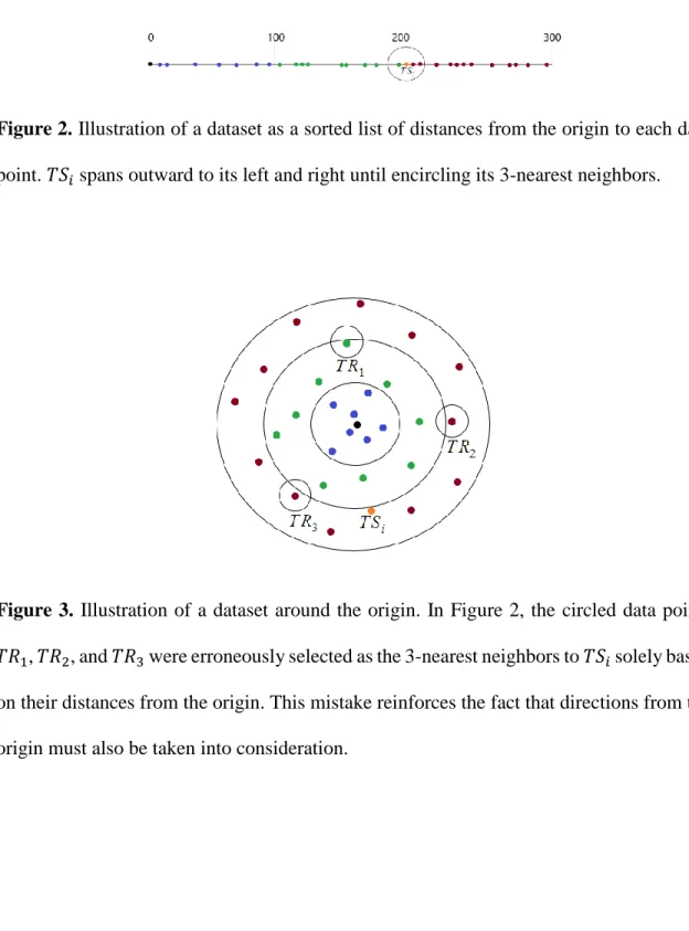
Figure 2. Illustration of a dataset as a sorted list of distances from the origin to each data point. 𝑇𝑆𝑖 spans outward to its left and right until encircling its 3-nearest neighbors.
Figure 3. Illustration of a dataset around the origin. In Figure 2, the circled data points 𝑇𝑅1, 𝑇𝑅2, and 𝑇𝑅3 were erroneously selected as the 3-nearest neighbors to 𝑇𝑆𝑖 solely based on their distances from the origin. This mistake reinforces the fact that directions from the origin must also be taken into consideration.
Figure 4. Illustration of a dataset around the origin. In this image, 𝑇𝑆𝑖 is correctly
encircling its 3-nearest neighbors.
Origin Creation
The first phase of the Bounded KNN algorithm is to create a data point to serve as the origin. Then, the algorithm needs to calculate the distance and direction between each data point and the origin. Using the formulas described in equations (3) and (4), we only need two data points to create a vector and compute its distance from the origin, or magnitude. Using the formula in equation (5), we can calculate the direction, or angle. However, it requires two vectors in order to produce a conclusive result. Therefore, we will create two origin data points, so that we can establish an origin vector between them.
11
The first origin will be a data point containing the average values for each feature in 𝑇𝑅, and it will be referenced as the mean origin, or 𝑂𝜇. For a more precise definition of
the mean origin, see equation (7). The second origin will be a data point containing the maximum values from each feature in 𝑇𝑅, and it will be referenced as the max origin, or 𝑂𝑚𝑎𝑥. For a more precise definition of the max origin, see equation (8). The vector created from connecting 𝑂𝜇 to 𝑂𝑚𝑎𝑥 will be referenced as the origin vector, or 𝑂⃗ .
The main purpose of the mean origin is to act as the source for all the vectors created, which includes magnitudes or distances. The main purpose of the origin vector is to serve as a point of reference for angle, or cosine similarity, calculations. It is important to note that the mean and max origins must be different data points. Otherwise, the origin vector would be a zero-magnitude vector and we would be unable to perform cosine similarity calculations. However, as long as the training dataset contains at least two different samples, this situation should never arise.
𝑂𝜇 = ( ∑ 𝑇𝑅𝑗1 𝑠𝑖𝑧𝑒(𝑇𝑅) 𝑗=1 𝑠𝑖𝑧𝑒(𝑇𝑅) , ∑𝑠𝑖𝑧𝑒(𝑇𝑅)𝑗=1 𝑇𝑅𝑗2 𝑠𝑖𝑧𝑒(𝑇𝑅) , … , ∑𝑠𝑖𝑧𝑒(𝑇𝑅)𝑗=1 𝑇𝑅𝑗𝑝 𝑠𝑖𝑧𝑒(𝑇𝑅) ) (7)
𝑂𝑚𝑎𝑥 = ( max(𝑇𝑅𝑗1), max(𝑇𝑅𝑗2), … , max(𝑇𝑅𝑗𝑝) ) (8)
Now that we have defined 𝑂𝜇 and 𝑂⃗ , we can proceed to the second phase, which is the model creation. The model consists of two lists: a list of vector objects sorted by angle and then by magnitude, and a list of neighbor objects sorted by magnitude. The vector model is a collection of all the vectors created to each sample in 𝑇𝑅. To be precise, 𝑂𝜇 will
serve as the source for all vectors created to each 𝑇𝑅𝑗. The distance between 𝑂𝜇 and 𝑇𝑅𝑗 is equal to the magnitude of their vector, i.e. ‖𝑂⃗⃗⃗⃗⃗⃗⃗⃗⃗⃗⃗⃗ ‖𝜇𝑇𝑅𝑗 . We define the direction from 𝑂𝜇 to 𝑇𝑅𝑗 as the angle between 𝑂⃗ and 𝑂⃗⃗⃗⃗⃗⃗⃗⃗⃗⃗⃗⃗ 𝜇𝑇𝑅𝑗. In rare cases where a training sample is equal to
𝑂𝜇, the resulting zero-magnitude vector will have a magnitude of zero and a null angle.
Once all vectors have been added to the model, the model is sorted by angle and then by magnitude in ascending order. Vectors with a null angle are inserted at the front of the vector model.
Each time a vector object is created, a neighbor object is also created and it copies the vector’s magnitude value in its distance attribute. The neighbor objects are added to the neighbor model and sorted by distance in ascending order. It is important to mention that the vector and neighbor models are reusable and do not need to be recreated. Table 1 demonstrates a possible representation of a dataset as a vector model.
13
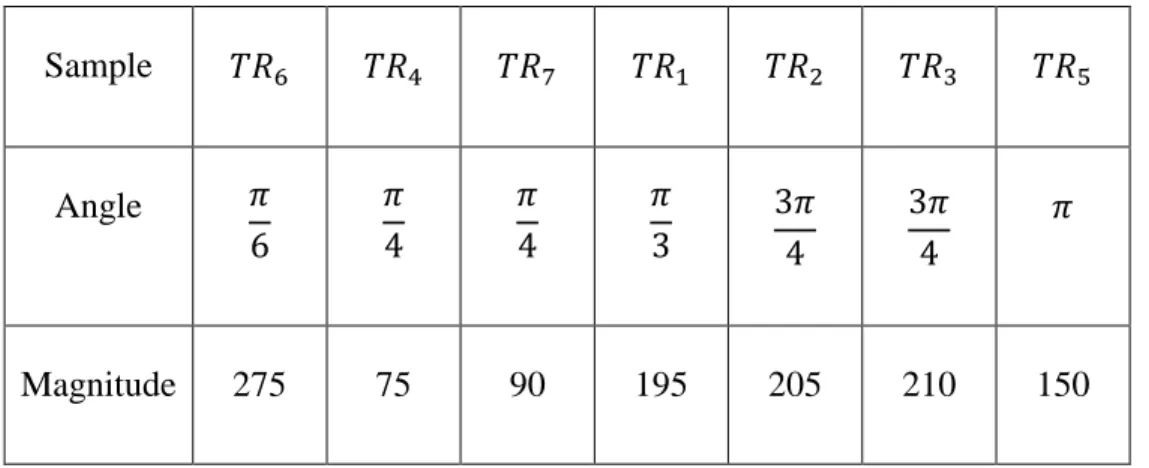
Table 1. Representation of a sorted vector model. The angle is the value between 𝑂⃗ and 𝑂𝜇𝑇𝑅𝑗
⃗⃗⃗⃗⃗⃗⃗⃗⃗⃗⃗⃗ , and the magnitude is ‖𝑂⃗⃗⃗⃗⃗⃗⃗⃗⃗⃗⃗⃗ ‖𝜇𝑇𝑅𝑗 . The model is sorted by angle and then by magnitude in ascending order. Sample 𝑇𝑅6 𝑇𝑅4 𝑇𝑅7 𝑇𝑅1 𝑇𝑅2 𝑇𝑅3 𝑇𝑅5 Angle 𝜋 6 𝜋 4 𝜋 4 𝜋 3 3𝜋 4 3𝜋 4 𝜋 Magnitude 275 75 90 195 205 210 150
Table 2. Representation of a sorted neighbor model. The distance is equivalent to the respective vector’s magnitude value. The model is sorted by distance in ascending order.
Sample 𝑇𝑅4 𝑇𝑅7 𝑇𝑅5 𝑇𝑅1 𝑇𝑅2 𝑇𝑅3 𝑇𝑅6
Nearest Neighbor Search
The third and final phase is to find the 𝐾 nearest neighbors to a given 𝑇𝑆𝑖. The Bounded KNN algorithm maintains dynamic angle and magnitude boundaries to restrict the nearest neighbor search, which leads to a reduction in the number of comparisons. The angle boundary is initially set to 𝜋, which allows all vectors to be evaluated since the angle values given in equation (5) range from 0 to 𝜋 radians. Similarly, the magnitude boundary is initially set to positive infinity in order to allow evaluation of all vectors. We also initialize an empty list to hold 𝑇𝑆𝑖’s nearest neighbors, let’s refer to it as 𝑁𝑁𝑖.
The nearest neighbor search begins by creating a vector from 𝑂𝜇 to 𝑇𝑆𝑖 and calculating its magnitude as well as its angle from 𝑂⃗ . In rare cases where 𝑂⃗⃗⃗⃗⃗⃗⃗⃗⃗⃗⃗ 𝜇𝑇𝑆𝑖 is a zero-magnitude vector, the 𝐾 nearest neighbors can be found by simply fetching the first 𝐾 neighbors in the neighbor model. The common case is to proceed with the following instructions.
1) Find the insertion index of 𝑂⃗⃗⃗⃗⃗⃗⃗⃗⃗⃗⃗ 𝜇𝑇𝑆𝑖 in the vector model. This can be accomplished via a binary search since the vector model was previously sorted.
2) Assign left and right pointers equal to the vector objects before and after the insertion index in the vector model. More precisely, the left pointer is equal to the 𝑖𝑛𝑠𝑒𝑟𝑡𝑖𝑜𝑛 𝑖𝑛𝑑𝑒𝑥 − 1, and the right pointer is equal to the 𝑖𝑛𝑠𝑒𝑟𝑡𝑖𝑜𝑛 𝑖𝑛𝑑𝑒𝑥
15
3) Determine whether the left or right vector is closer to 𝑂⃗⃗⃗⃗⃗⃗⃗⃗⃗⃗⃗ 𝜇𝑇𝑆𝑖 by comparing angle differences. In the case of a tie, we compare magnitude differences. The closer vector will be referred to as 𝐶𝑉⃗⃗⃗⃗⃗ .
4) If the left pointer was referencing 𝐶𝑉⃗⃗⃗⃗⃗ , decrement the left pointer. Otherwise, increment the right pointer.
5) If 𝑠𝑖𝑧𝑒(𝑁𝑁𝑖) < 𝐾, insert 𝐶𝑉⃗⃗⃗⃗⃗ into 𝑁𝑁𝑖 in ascending order by angle, then by magnitude. When 𝑠𝑖𝑧𝑒(𝑁𝑁𝑖) reaches 𝐾, update the angle and magnitude boundaries as described in Figure 5.
6) If 𝑠𝑖𝑧𝑒(𝑁𝑁𝑖) ≥ 𝐾, we verify that 𝐶𝑉⃗⃗⃗⃗⃗ is within our angle and magnitude boundaries. That is, verify that the angle between 𝐶𝑉⃗⃗⃗⃗⃗ and 𝑂⃗ is within 𝜃 ± 𝜃𝑏𝑜𝑢𝑛𝑑, and that ‖𝐶𝑉⃗⃗⃗⃗⃗ ‖
is within ‖𝑂⃗⃗⃗⃗⃗⃗⃗⃗⃗⃗⃗ ‖ ± 𝑟𝜇𝑇𝑆𝑖 . Then, we must perform an additional check to verify that the angle between 𝐶𝑉⃗⃗⃗⃗⃗ and 𝑂⃗⃗⃗⃗⃗⃗⃗⃗⃗⃗⃗ 𝜇𝑇𝑆𝑖 is indeed within the angle boundaries. For a
detailed explanation of this requirement, see Figure 6. Once verified, we find the magnitude of the connecting vector between 𝐶𝑉⃗⃗⃗⃗⃗ and 𝑂⃗⃗⃗⃗⃗⃗⃗⃗⃗⃗⃗ 𝜇𝑇𝑆𝑖. If the magnitude of the
connecting vector is less than 𝑟, insert 𝐶𝑉⃗⃗⃗⃗⃗ into 𝑁𝑁𝑖 in ascending order by angle and then by magnitude, and remove the last element in 𝑁𝑁𝑖. Finally, update the angle and magnitude boundaries as described in Figure 5.
7) Repeat steps 3-6 until both left and right pointers reference vectors which are outside of the angle boundaries, or both pointers are null.
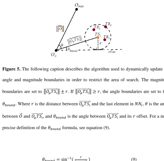
Figure 5. The following caption describes the algorithm used to dynamically update the angle and magnitude boundaries in order to restrict the area of search. The magnitude boundaries are set to ‖𝑂⃗⃗⃗⃗⃗⃗⃗⃗⃗⃗⃗ ‖ ± 𝑟𝜇𝑇𝑆𝑖 . If ‖𝑂⃗⃗⃗⃗⃗⃗⃗⃗⃗⃗⃗ ‖ ≥ 𝑟𝜇𝑇𝑆𝑖 , the angle boundaries are set to 𝜃 ±
𝜃𝑏𝑜𝑢𝑛𝑑. Where 𝑟 is the distance between 𝑂⃗⃗⃗⃗⃗⃗⃗⃗⃗⃗⃗ 𝜇𝑇𝑆𝑖 and the last element in 𝑁𝑁𝑖, 𝜃 is the angle between 𝑂⃗ and 𝑂⃗⃗⃗⃗⃗⃗⃗⃗⃗⃗⃗ 𝜇𝑇𝑆𝑖, and 𝜃𝑏𝑜𝑢𝑛𝑑 is the angle between 𝑂⃗⃗⃗⃗⃗⃗⃗⃗⃗⃗⃗ 𝜇𝑇𝑆𝑖 and its 𝑟 offset. For a more precise definition of the 𝜃𝑏𝑜𝑢𝑛𝑑 formula, see equation (9).
𝜃𝑏𝑜𝑢𝑛𝑑 = sin−1( 𝑟
17
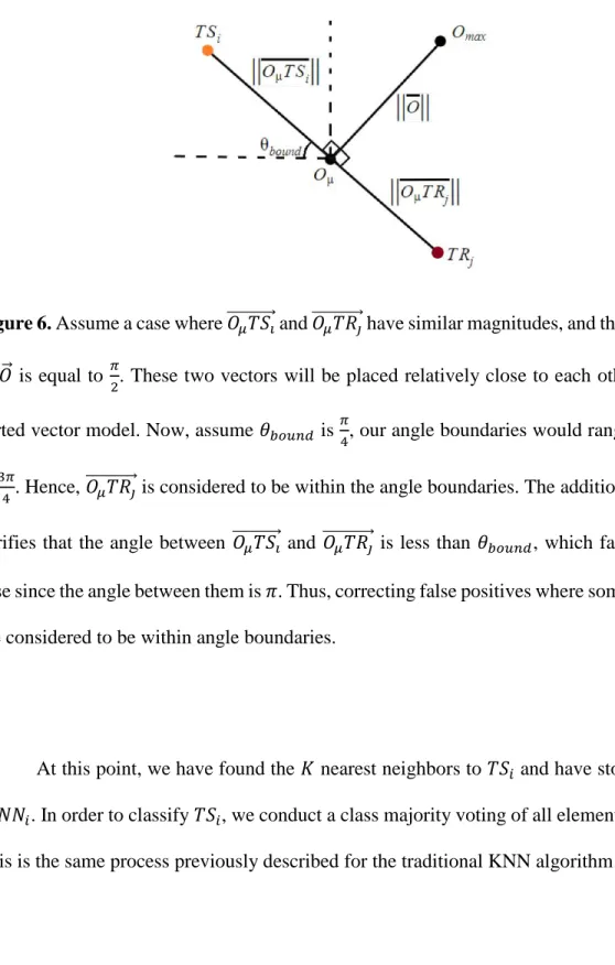
Figure 6. Assume a case where 𝑂⃗⃗⃗⃗⃗⃗⃗⃗⃗⃗⃗ 𝜇𝑇𝑆𝑖 and 𝑂⃗⃗⃗⃗⃗⃗⃗⃗⃗⃗⃗⃗ 𝜇𝑇𝑅𝑗 have similar magnitudes, and their angles
to 𝑂⃗ is equal to 𝜋
2. These two vectors will be placed relatively close to each other in the
sorted vector model. Now, assume 𝜃𝑏𝑜𝑢𝑛𝑑 is 𝜋
4, our angle boundaries would range from 𝜋 4
to 3𝜋
4. Hence, 𝑂⃗⃗⃗⃗⃗⃗⃗⃗⃗⃗⃗⃗ 𝜇𝑇𝑅𝑗 is considered to be within the angle boundaries. The additional check
verifies that the angle between 𝑂⃗⃗⃗⃗⃗⃗⃗⃗⃗⃗⃗ 𝜇𝑇𝑆𝑖 and 𝑂⃗⃗⃗⃗⃗⃗⃗⃗⃗⃗⃗⃗ 𝜇𝑇𝑅𝑗 is less than 𝜃𝑏𝑜𝑢𝑛𝑑, which fails in this
case since the angle between them is 𝜋. Thus, correcting false positives where some vectors are considered to be within angle boundaries.
At this point, we have found the 𝐾 nearest neighbors to 𝑇𝑆𝑖 and have stored them in 𝑁𝑁𝑖. In order to classify 𝑇𝑆𝑖, we conduct a class majority voting of all elements in 𝑁𝑁𝑖. This is the same process previously described for the traditional KNN algorithm.
Chapter V
Bounded KNN and Spark
The next step in our research was to migrate the Bounded KNN algorithm onto Spark to observe its applicability in the field of Big Data. The following sections will cover the details of the Bounded KNN’s Spark implementation. The training and test datasets were loaded from our Hadoop Distributed File System (HDFS) as Resilient Distributed Datasets (RDDs). All function operations, also known as transformations on Spark, performed on an RDD are parallelized across all the worker nodes in the cluster. We take advantage of this fact to parallelize the three phases of our Bounded KNN algorithm and further improve its performance benefits in the field of Big Data.
Parallel Origin Creation
The first phase is to create the mean origin, max origin, and origin vector. Finding the mean and max origins was challenging at first. There are built-in mean and max transformation functions for RDDs, but they operate on one multi-dimensional sample
19
rather than on one column across multiple samples. To get around this, we split the dimensions of our dataset and assign an index value to each one. Thus, our initial output on Spark was a features RDD containing a list of key-value pairs consisting of the column index as the key and the column value as the value.
To create the mean origin, the features RDD was reduced by key and the values were added together. We then apply a transformation to divide each key, which is a sum of all the column values, by the total number of samples. The final result is a sample containing the average of each column in the dataset. To create the max origin, the features RDD was reduced by key, similarly to the mean origin, but we keep the max value instead of adding them together. The final result is a sample containing the maximum values for each column in the dataset. Lastly, we create the origin vector by utilizing the mean and max origins in the same way it was done on the local version of the Bounded KNN.
Parallel Model Creation
The mean origin and the origin vector are shared from the driver node to the worker nodes via broadcast variables, therefore allowing the worker nodes to have a read-only copy of those variables. This step is necessary because the mean origin is crucial in creating the training vectors and the origin vector is crucial in calculating the cosine similarities. Next, we apply a map transformation on the training dataset RDD to create the model. The map transformation allows us to execute a custom function on each element in the RDD.
The custom function executed returns a model RDD, which consists of a list of key-value pairs. It initially contains two entries: a vector key with a training vector object, and a neighbor key with a training neighbor object. The model RDD is then reduced by key, which ends up combining all the vector objects into one list and all the neighbor objects into another list. Lastly, the model’s list of vectors is sorted by angle and then by magnitude, while the model’s list of neighbors is sorted by distance.
Parallel Nearest Neighbor Search
The last phase consists of finding the nearest neighbors to each test sample. In order to accomplish this, we need to share the model RDD, which was created in the previous phase, with the worker nodes via a broadcast variable. Then, we leverage the map transformation to perform a custom function on the test dataset RDD. This custom function results in a list of vector objects created from the mean origin to each test sample. Finally, we apply another custom function to these results, which simply performs the nearest neighbor search function from the local Bounded KNN implementation on each of these vectors.
21
Chapter VI
Experiments
We decided to use the MNIST dataset for our experiments. It is an easily understandable dataset which contains multiple samples to choose from. The dataset was split into subsets of various sizes to observe scalability and performance differences between the traditional KNN and Bounded KNN algorithms. We also compared the performance difference between the Bounded KNN locally and the Bounded KNN on Spark. The performance measurements we focused on were prediction accuracy and run-time in seconds. The algorithms were implemented in Python 2.7 both locally and on Spark. The Spark cluster contained 8 worker nodes, each with 16GB RAM.
MNIST Dataset
The MNIST dataset contains images of handwritten digits, and is commonly used for training image processing systems. Each sample represents a 28x28 grayscale image of a handwritten digit ranging from 0 to 9. There are 784 features to represent the pixel values
in the image, which range from 0 to 255, and one additional feature to indicate the class this image belongs to. Thus, the dimensionality of this dataset is 785.
Traditional KNN vs. Bounded KNN
We created four subsets of the MNIST dataset. The training datasets ranged from 950 to 9500 samples, and the test datasets ranged from 50 to 500 samples. Each subset was classified using both algorithms and with different values of 𝐾. The experiments were repeated at least five times, and the run-time values represent the best result for each value of 𝐾. The following Tables 3-6 show a side-by-side comparison of the prediction accuracy and run-time results for the traditional KNN and the Bounded KNN algorithms on each dataset. The graph in Figure 7 compares scalability of the two algorithms by plotting the average run-time results for each dataset as the number of samples increases.
23
Table 3. Comparison of traditional KNN vs. Bounded KNN using 950 training samples and 50 test samples.
𝐾 Traditional Accuracy Bounded Accuracy Traditional Run-Time Bounded Run-Time 1 88.00% 88.00% 18.33 0.865 3 94.00% 94.00% 18.393 0.959 5 90.00% 90.00% 18.214 1.045 7 88.00% 88.00% 18.217 1.04 9 88.00% 88.00% 18.407 1.082 11 86.00% 86.00% 18.315 1.155 13 84.00% 84.00% 18.414 1.098 15 82.00% 82.00% 18.71 1.122 AVG 87.50% 87.50% 18.375 1.046
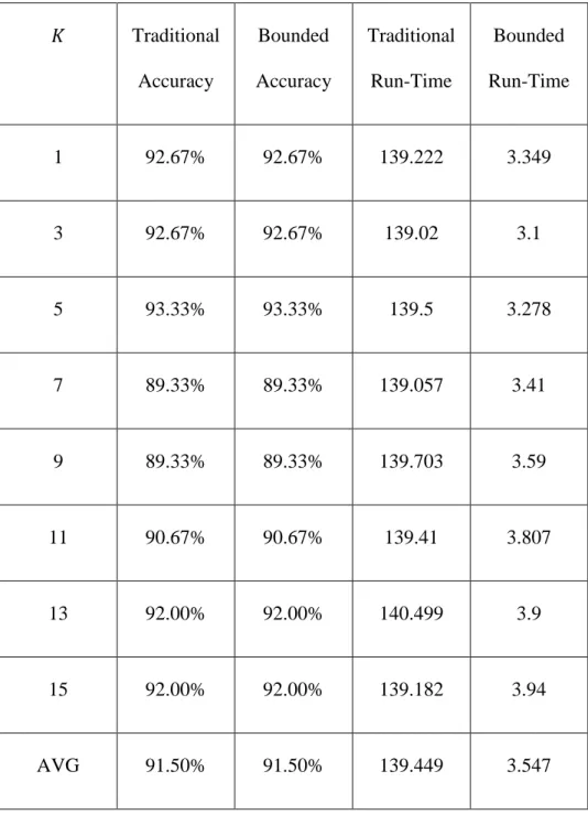
Table 4. Comparison of traditional KNN vs. Bounded KNN using 2350 training samples and 150 test samples.
𝐾 Traditional Accuracy Bounded Accuracy Traditional Run-Time Bounded Run-Time 1 92.67% 92.67% 139.222 3.349 3 92.67% 92.67% 139.02 3.1 5 93.33% 93.33% 139.5 3.278 7 89.33% 89.33% 139.057 3.41 9 89.33% 89.33% 139.703 3.59 11 90.67% 90.67% 139.41 3.807 13 92.00% 92.00% 140.499 3.9 15 92.00% 92.00% 139.182 3.94 AVG 91.50% 91.50% 139.449 3.547
25
Table 5. Comparison of traditional KNN vs. Bounded KNN using 4700 training samples and 300 test samples.
𝐾 Traditional Accuracy Bounded Accuracy Traditional Run-Time Bounded Run-Time 1 94.33% 94.33% 563.371 8.231 3 95.33% 95.33% 561.231 8.901 5 95.33% 95.33% 562.965 9.501 7 94.67% 94.67% 562.12 9.87 9 95.00% 95.00% 563.604 10.517 11 93.67% 93.67% 557.688 11.68 13 93.67% 93.67% 551.655 11.33 15 93.67% 93.67% 549.181 11.44 AVG 94.46% 94.46% 558.977 10.184
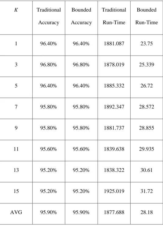
Table 6. Comparison of traditional KNN vs. Bounded KNN using 9500 training samples and 500 test samples.
𝐾 Traditional Accuracy Bounded Accuracy Traditional Run-Time Bounded Run-Time 1 96.40% 96.40% 1881.087 23.75 3 96.80% 96.80% 1878.019 25.339 5 96.40% 96.40% 1885.332 26.72 7 95.80% 95.80% 1892.347 28.572 9 95.80% 95.80% 1881.737 28.855 11 95.60% 95.60% 1839.638 29.935 13 95.20% 95.20% 1838.322 30.61 15 95.20% 95.20% 1925.019 31.72 AVG 95.90% 95.90% 1877.688 28.18
27
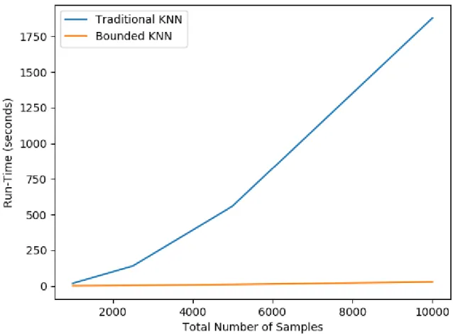
Figure 7. Comparison of the run-time for both the traditional KNN and Bounded KNN algorithms on different sized datasets.
From these results, we can see that the Bounded KNN outperforms the traditional KNN on all datasets. It reduced execution time of the smallest dataset by 94.31%, and grows up to a 98.45% reduction for the largest dataset. The increasing performance gap between the two algorithms, as can be observed in Figure 7, indicates that the benefits continuously scale along with the datasets. Furthermore, the Bounded KNN algorithm
produces the same nearest neighbors as the traditional KNN algorithm for any given test sample, which allows us to preserve the algorithm’s accuracy.
Local Bounded KNN vs. Spark Bounded KNN
We ran the Bounded KNN Spark implementation on the same datasets described above and compared its results to the local implementation of the Bounded KNN algorithm. However, since Spark is more suited to handling large amounts of data, we created two larger subsets of the data. The first subset contains 18000 training samples and 2000 test samples, and the second subset contains 27000 training samples and 3000 test samples. This allows us to more accurately compare the local and Spark implementations of the Bounded KNN algorithm.
29
Table 7. Comparison of the local implementation of the Bounded KNN vs. the Spark implementation of the Bounded KNN using 950 training samples and 50 test samples.
𝐾 Spark Accuracy Local Accuracy Spark Run-Time Local Run-Time 1 88.00% 88.00% 19.052 0.865 3 94.00% 94.00% 17.903 0.959 5 90.00% 90.00% 18.376 1.045 7 88.00% 88.00% 18.001 1.04 9 88.00% 88.00% 17.812 1.082 11 86.00% 86.00% 18.433 1.155 13 84.00% 84.00% 18.33 1.098 15 82.00% 82.00% 18.068 1.122 AVG 87.50% 87.50% 18.247 1.046
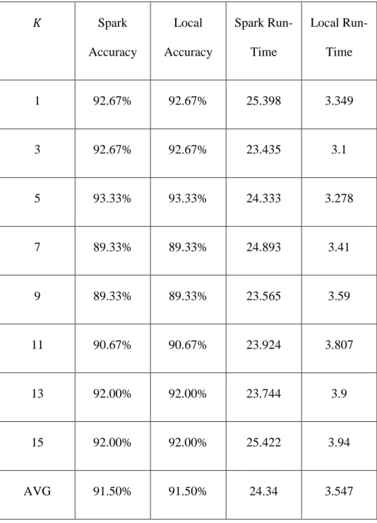
Table 8. Comparison of the local implementation of the Bounded KNN vs. the Spark implementation of the Bounded KNN using 2350 training samples and 150 test samples.
𝐾 Spark Accuracy Local Accuracy Spark Run-Time Local Run-Time 1 92.67% 92.67% 25.398 3.349 3 92.67% 92.67% 23.435 3.1 5 93.33% 93.33% 24.333 3.278 7 89.33% 89.33% 24.893 3.41 9 89.33% 89.33% 23.565 3.59 11 90.67% 90.67% 23.924 3.807 13 92.00% 92.00% 23.744 3.9 15 92.00% 92.00% 25.422 3.94 AVG 91.50% 91.50% 24.34 3.547
31
Table 9. Comparison of the local implementation of the Bounded KNN vs. the Spark implementation of the Bounded KNN using 4700 training samples and 300 test samples.
𝐾 Spark Accuracy Local Accuracy Spark Run-Time Local Run-Time 1 94.33% 94.33% 32.545 8.231 3 95.33% 95.33% 31.983 8.901 5 95.33% 95.33% 33.108 9.501 7 94.67% 94.67% 37.06 9.87 9 95.00% 95.00% 33.449 10.517 11 93.67% 93.67% 34.111 11.68 13 93.67% 93.67% 33.674 11.33 15 93.67% 93.67% 32.511 11.44 AVG 94.46% 94.46% 29.487 10.184
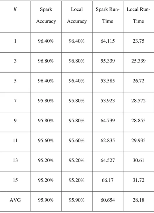
Table 10. Comparison of the local implementation of the Bounded KNN vs. the Spark implementation of the Bounded KNN using 9500 training samples and 500 test samples.
𝐾 Spark Accuracy Local Accuracy Spark Run-Time Local Run-Time 1 96.40% 96.40% 64.115 23.75 3 96.80% 96.80% 55.339 25.339 5 96.40% 96.40% 53.585 26.72 7 95.80% 95.80% 53.923 28.572 9 95.80% 95.80% 64.739 28.855 11 95.60% 95.60% 62.835 29.935 13 95.20% 95.20% 64.527 30.61 15 95.20% 95.20% 66.17 31.72 AVG 95.90% 95.90% 60.654 28.18
33
Table 11. Comparison of the local implementation of the Bounded KNN vs. the Spark implementation of the Bounded KNN using 18000 training samples and 2000 test samples.
𝐾 Spark Accuracy Local Accuracy Spark Run-Time Local Run-Time 1 96.90% 96.90% 149.641 150.79 3 96.70% 96.70% 148.849 156.675 5 96.30% 96.30% 153.002 164.106 7 96.05% 96.05% 147.032 169.369 9 95.75% 95.75% 151.049 174.632 11 95.50% 95.50% 163.058 178.727 13 95.50% 95.50% 165.101 184.636 15 95.20% 95.20% 163.899 181.016 AVG 95.99% 95.99% 155.204 169.99
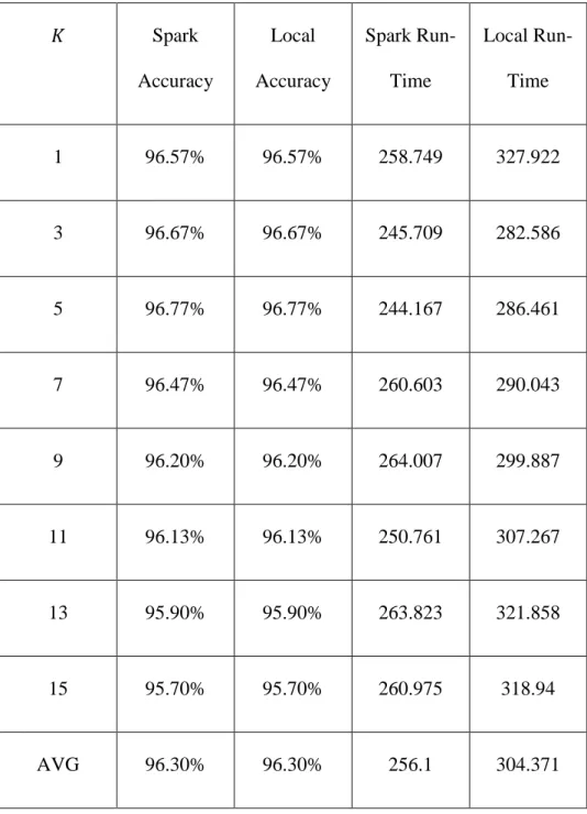
Table 12. Comparison of the local implementation of the Bounded KNN vs. the Spark implementation of the Bounded KNN using 27000 training samples and 3000 test samples.
𝐾 Spark Accuracy Local Accuracy Spark Run-Time Local Run-Time 1 96.57% 96.57% 258.749 327.922 3 96.67% 96.67% 245.709 282.586 5 96.77% 96.77% 244.167 286.461 7 96.47% 96.47% 260.603 290.043 9 96.20% 96.20% 264.007 299.887 11 96.13% 96.13% 250.761 307.267 13 95.90% 95.90% 263.823 321.858 15 95.70% 95.70% 260.975 318.94 AVG 96.30% 96.30% 256.1 304.371
35
Figure 8. Comparison of the local implementation of the Bounded KNN vs. the Spark implementation of the Bounded KNN on different sized datasets.
For the first four datasets, the local implementation of the Bounded KNN outperforms the Spark implementation. This is due to the overhead time associated with distributing the processing to all the worker nodes in the Spark cluster. However, the Spark implementation continuous to close the gap as the size of the datasets increases. As
demonstrated on the last two datasets, the Spark implementation of the Bounded KNN algorithm eventually catches up and outperforms the local implementation.
Next, let’s further analyze the performance difference between the two implementations for each dataset. For the 1K samples dataset, the Spark implementation was 1644.46% slower. For the 2.5K samples dataset, the Spark implementation was 586.21% slower. For the 5K samples dataset, the Spark implementation was 189.54% slower. For the 10K samples dataset, the Spark version was 115.24% slower. For the 20K samples dataset, the Spark version was 8.7% faster. Finally, for the 30K samples dataset, the Spark version was 15.86% faster. Assuming that this trend continues, it is safe to assume that the Spark version will provide a significant performance boost to the algorithm when handling the large datasets which are prevalent in the field of Big Data.
Chapter VII
Conclusion
In this paper, we presented the Bounded KNN algorithm, which is an optimization to the traditional KNN algorithm that leverages vector space models. It creates a different representation of the data, which allows us to take advantage of vector related mathematical
37
properties. Since all vectors spawn from the mean origin and hold an angle reference to the origin vector, the creation of the origin data points and the origin vector serve as the enabling factor and backbone of our algorithm. The Bounded KNN algorithm yields significant performance improvements over the traditional KNN algorithm, in terms of run-time, while preserving the algorithm’s accuracy. These benefits are further improved by parallelizing the Bounded KNN on Spark, which distributes the work among a cluster of machines. Therefore, concluding that these solutions provide us with a better approach to handle today’s increasingly large datasets.
References
[1] Cai, Y., Ji, D., & Cai, D.: A KNN Research Paper Classification Method Based on Shared Nearest Neighbor (2010).
[2] Rahal, I., & Perrizo, W.: An Optimized Approach for KNN Text Categorization using P-trees (2004).
[3] Guo, G., Wang, H., Bell, D., Bi, Y., & Greer, K.: KNN Model-Based Approach in Classification (2003).
[4] Dong, T., Cheng, W., & Shang, W.: The Research of kNN Text Categorization Algorithm Based On Eager Learning (2012).
[5] Jin, Z., Zhang, D., Hu, Y., Lin, S., Cai, D., & He, X.: Fast and Accurate Hashing Via Iterative Nearest Neighbors Expansion (2014).
[6] Zhang, Y., Huang, K., Geng, G., & Liu, C.: Fast kNN Graph Construction with Locality Sensitive Hashing (2013).
[7] Choi, D., & Chung, C.: Nearest Neighborhood Search in Spatial Databases (2015).
[8] Muja, M., & Lowe, D.: Scalable Nearest Neighbor Algorithms for High Dimensional Data (2014).
[9] Tang, J., Liu, J., Zhang, M., & Mei, Q.: Visualizing Large-scale and High-dimensional Data (2016).
39
[10] Bernhardsson, E. (2015, September 24). Nearest neighbor methods and vector models – part 1. Retrieved from https://erikbern.com/2015/09/24/nearest-neighbor-methods-vector-models-part-1.html
[11] Bernhardsson, E. (2015, October 1). Nearest neighbors and vector models – part 2 – algorithms and data structures. Retrieved from https://erikbern.com/2015/10/01/nearest-neighbors-and-vector-models-part-2-how-to-search-in-high-dimensional-spaces.html
[12] Maillo, J., Triguero, I., & Herrera, F.: A MapReduce-based k-Nearest Neighbor Approach for Big Data Classification (2015).
[13] Zhu, P., Zhan, X., & Qiu, W.: Efficient k-Nearest Neighbors Search in High Dimensions using MapReduce (2015).
[14] Lu, W., Shen, Y., Chen, S., & Ooi, B.: Efficient Processing of k Nearest Neighbor Joins using MapReduce (2012).
[15] Anchalia, P., & Roy, K.: The k-Nearest Neighbor Algorithm Using MapReduce Paradigm (2014).