Pricing of Basket Default Swaps Based on Factor Copulas and NIG

Procedia Computer Science 55 ( 2015 ) 566 – 574

1877-0509 © 2015 Published by Elsevier B.V. This is an open access article under the CC BY-NC-ND license (http://creativecommons.org/licenses/by-nc-nd/4.0/).

Peer-review under responsibility of the Organizing Committee of ITQM 2015 doi: 10.1016/j.procs.2015.07.046

ScienceDirect

Information Technology and Quantitative Management (ITQM2015)

Pricing of Basket Default Swaps Based on Factor Copulas and

NIG

*

Ping Li

1†

_{, Jie Liu}

1

_,

_Xinyun

_Zhang

1

_{, Guangdong Huang}

2 1_{School of Economics and Management, Beihang University, Beijing 100191, China}

2_{School of Science, China University of Geosciences, Beijing 100083, China}

Abstract

Due to the European debt crisis, the credit default swap (CDS) has been brought back to the spotlight of the financial market. At the meantime, the basket default swaps (BDS) emerges as the hottest issue amid the growing researches about CDS. It is extremely significant to define the correlations between the underlying assets and the default time. The copula approach can accurately specify the joint distribution. In this paper, the factors affecting the company’s valuation are classified into systematic factors and non-systematic factors. The fact-based statistics are utilized to analyze the distribution of systematic factors. Then we obtain the samples’ default information from the bond market and the correlation of the samples from stock market. We use the factor copula model to simulate the whole sample’s distribution and the correlation between the underlying assets, and then give the price for a BDS.

Keywords: Factor copula; Credit VaR; Principal component analysis

1.Introduction

The European debt crisis draws the world’s attention back to CDS. Basket Default Swaps (BDS) which is a basket of CDS is a kind of multi-name credit derivative, so it is important to characterize the correlations between the underlying assets and the default time.

In the factor model proposed by Vasicek (1987), the individual’s value in the credit portfolio is determined by two factors: the systemic factor and the individual factor. Gregory and Laurent (2002) extended Vasicek’s model, taking different individuals’ heterogeneous correlation with systemic factor into account, and studied credit portfolio’s correlation structure, spread and pricing. Then they proposed a two-factor model in 2004, studying the correlation between default time and default recovery based on the two-factor model and conducted simulation analysis. Burtschell, Gregory and Laurent (2005) compared several kinds of copula function (Gaussian copula, t-copula, Clayton copula) to describe joint default structure based on the factor

* _{This work was supported by the Natural Science Foundation of China (No. 71271015, 70971006), and the Fundamental Research Funds}

for Central Universities of China (No. 2652013106). † Corresponding author. Email: [email protected]

model and found that copula functions above behave similar in credit derivatives pricing. Li (2000) using the Gaussian Copula function to describe the default correlation, followed by Hull and White (2001) proposing a study of multi-asset correlations caused by the default risk model. Zhou etc (2006) applied approximate analysis in Monte Carlo simulation to price a BDS.

In this paper, we describe the default correlation between the underlying assets in the basket based on factor copula model and price a BDS by conditional default probability. The remaining of the paper are arranged as follows: Section 2 describes factor copula model; Section 3 gives the pricing model and process for a first-to-default swaps, and then in Section 4 we firstly obtain the systemic factor from empirical data analysis and then give a numerical example of BDS pricing based on single-factor Gaussian-NIG-copula model. In Section 5 we give the sensitivity analysis of the model parameters, and then in Section 6 we conclude the paper.

2.The Factor copula model

In Vasicek (1987)’s model they consider n debtors in a portfolio and assume that debt i’s value

V t

i

( )

_is affected by two factors: the systematic factor Y and the individual factor

H

i_{. Y and}

H

i _{are independent and with} expectations of 0 and variance of 1. They are related by the parameter

U

:

2

( )

1

,

1,...,

i i

V t

U

Y

U H

i

n

2

_,

( ( ), ( ))=

1,

i j

i

j

Cov V t V t

i

j

U

­

z

®

¯

When a company is insolvent it will default. The occurrence of the default event can be described as:

i i

V

H

If firm i’s unconditional default probability is known as pi, then the asset level which decides whether defaults or not will be Hi Gi1( )pi _{, then we can get debt i’s conditional default probability when Y=y:}

1 2 2

( )

(

|

)

(

|

)

(

)

1

1

i i i i i i i i i i

H

Y

G

p

y

P V

H Y

y

P

H

U

Y

y

H

U

U

U

d

3. BDS Pricing Model

The BDS is an insurance contract for the occurrence of some corporations’ default. BDS can be divided into multiple and disposable default protection portfolio. First-to-default swaps mean that when any asset in the basket defaults, the contract terminates and the protection seller bears the default risk.

Under risk neutral probability, the present value of the loss when default occurs equal to the present value of the premium paid by the buyer. Under complete market and risk-neutral assumption, according to breakeven and arbitrage principle, we plus all the present value of buyers’ spread and the present value of contingent compensation, then we solve the equation and get the breakeven default swaps spreads Sk.

Under risk neutral measure, we calculate the present value of the premium payment leg (PL):

^

`

1 1

(

,

) (0, ) [

k

]

j n k j j j _t j

PL S F

¦

'

t

'

t B

t E l

_{W !} (1) where, 1 n i i F

¦

F

is the total face value of the portfolio, _Wk _{is the default time of asset k,} {k }

j

t

l

_{W !}

is the indicator function of a credit event using risk neutral measure.

During the contract period, if the kth_{asset in the portfolio defaults, the contract’s seller needs to pay} (1

i i

F R˅ _{to the protection buyer of asset k . The present value of this default payment leg (DL) is}

1 { }

(1

) [ (0, )

k

]

i n k i i i

F

R E B

l

DL

¦

W

_{W W} (2)

According to no arbitrage theory we can get the fair spread

S

k _{of a BDS from PL=DL:}

k j 1 } 1 { } 1 _{{τ t}

(1

) [ (0, )

]

(

,

)

(0, )

[

]

k i n k i i m j i j j j k

F

R E B

l

t

t

B

t E l

S

W W

W

_!

'

¦

¦

(3)

In formula (3), the default time of the underlying assets is the key problem. In this paper, we use reduced-form model and factor copula model to describe the correlation between the default times. We need to know two things: the marginal and joint distributions of the default times. In the reduced form model the default intensity is assumed to be horizontal. Based on the model, we can get marginal distributions of the default times.

4. Numerical Pricing

4.1. Empirical analysis for systematic factors

The pricing process in Section 3 is based on the hypothesis that the systematic factor has the normal distribution. In this section we use principal component analysis to generate the systematic factor and see if it has the normal distribution. We take Shanghai Composite Index (

V

1_{), macroeconomic climate index (}

V

2_{), and M2} growth (

V

3_{) into consideration, and use the monthly data from January 2009 to December 2011.}

4.1.1 Correlation test

Firstly, we examine if the initial variables are suitable for factor analysis, namely whether there is a linear correlation between them. We obtain the correlation matrix as shown in Table 1.

Table 1. Correlation Matrix

V1 V2 V3 Correlation V1 1.000 .294 .306 V2 .294 1.000 .468 V3 .306 .468 1.000 Sig. (1-tailed) V1 .046 .039 V2 .046 .003 V3 .039 .003

From the table we can see that the values of Sig correlation coefficient are less than 0.05, indicating that these variables have obvious linear correlation and the factor analysis is necessary. If these variables have no linear correlation there is no sharing of information and it is not necessary to extract the common factor. Considering from an economic perspective, the degree of economic boom and the monetary policy will be reflected in the company's running, and this will inevitably be reflected through the stock index.

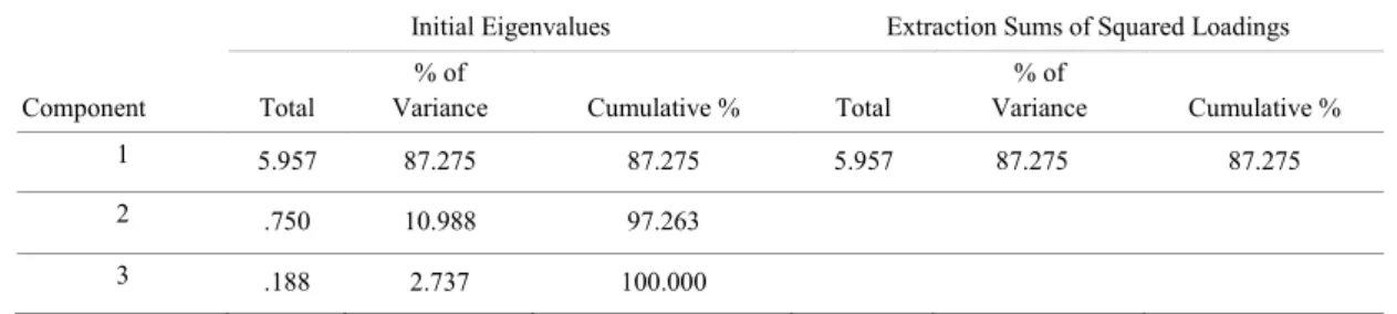
4.1.2 Variance Explanation

Then we do the variance explanation and the results are shown in Table 2. The criterion of selecting principal component’s number is that eigenvalues are greater than 1 and the cumulative proportion of explained variance is greater than 80%. From the table we can see that the factor extracted can explain 87.275% of the variance, so we think one factor is appropriate.

Table 2. Explained Variance

Component

Initial Eigenvalues Extraction Sums of Squared Loadings Total

% of

Variance Cumulative % Total

% of Variance Cumulative % 1 _{5.957 87.275 87.275 5.957 87.275 87.275} 2 _{.750 10.988 97.263} 3 _{.188 2.737 100.000} 4.1.3 Component Score

We also obtain the component score coefficient matrix as reported in Table 3. From the table we can get the systematic factor:

Systematic factor=0.388*

'

V

₁+0.462*

'

V

₂+0.466*

'

V

₃ (4) Table 3.Component Score Coefficient Matrix

Component 1

V1 .388

V2 .462

V3 .466

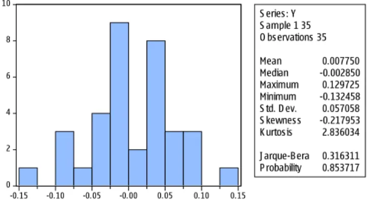
Then we can get the descriptive statistics of the systematic factor as shown in Figure 1, from which we can see that we cannot refuse that the systematic factor has normal distribution.

Fig 1 Descriptive statistics of the systematic factor

4.2 Pricing First-to-Default swaps based on single-factor copula model

The factor copula model above is based on the hypothesis that both systematic factor and the individual factor have normal distributions which leads the tail dependence problem. Now we suppose that individual factor has inverse Gaussian distribution NIG (2,1,4,6) while systematic factor has normal distribution N(0,0.05) as above.

We consider a BDS in which the underlying assets are corporate bonds issued by ten Chinese companies. The premium will be paid at the end of each year. The BDS is described as follows:

Table4. Items of the BDS

Maturity 2 years

Number of assets (N) 10

Face value of each asset (A) 10 million

Hazard function˄˄O˅˅ 0.01 Correlation coefficient (

U

) 0.3 0 2 4 6 8 10 -0.15 -0.10 -0.05 -0.00 0.05 0.10 0.15 S eries : Y S ample 1 35 O bs ervations 35 Mean 0.007750 Median -0.002850 Maximum 0.129725 Minimum -0.132458 S td. D ev. 0.057058 S kewnes s -0.217953 K urtos is 2.836034 J arque-Bera 0.316311 P robability 0.853717

Recovery rate (R) 0.4

Risk-free rate 0.05

Then we can calculate the fair spread of the BDS as follows:

1) Calculate each asset’s default distribution function ( )Q t and survival function ( )S t ; ( ) 1 exp( ) 1 exp( 0.01 1) 0.01, ( ) exp( ) 0.99 i i Q t t S t t

O

O

u

2) Obtain the default distribution fuction’s inverse value: x F Q t1[ ( )]i

1_[0.01_] 1_{(0.2) 0.5793}

0.05 x _{) )}

3) Calculate the conditional default probability under systematic factor Y and correlation coefficient

U

1 2 2 ( ) ( | ) ( | ) ( ) 1 1 i i i i i i i i i i H Y G p y P V H Y y PH U Y y H U U U d 0.5793 0 (0 | ) ( ) (0.6924) 0.0012 1 0.3 p Y H H

4) Using conditional default probability to calculate the probability distribution of default loss: 0, (0 | ) 1 (1| ) (1 0.0012)10 0.988 n i i K p Y

–

S Y 1

1

(1| )

0.0012

1, (1| )

(0 | )

0.988 10

0.012

(1| )

0.9988

n _i i i

S

Y

K

p

Y

p

Y

S

Y

u u

¦

where K is the number of assets in the basket which defaults. 5) Get the unconditional default distribution of K assets at time T: ( ) ( | ) ( ) ( ) p K

³

p K Y f Y d Y

( |

2) (

(

, 2])

...

( |

2) (

[ 1, 2])

( |

2) (

[ 2,

))

p K Y

f Y

Y

p K Y

f Y

Y

p K Y

f Y

Y

|

f '

'

f '

0.0017*0.0061*1 0.0047*0.1631*1 0.988*0.3019*1 0.0003*0.3019 0.0000*0.7240*1 0.2688

6) Get the probability distribution of K assets at t=1 Table 5 Distribution of K assets

K 0 1 2 3 4 5 6 7 …

t=1 0.27 0.19 0.05 0.04 0.02 0.01 0.0 * *

7) Calculate the expected loss (EL) of each tranche: Table 6 Expected loss (EL)

Number of default assets˄K˅ Loss L=K*A*(1-R) EL˄t=1˅ 0 0 0 1 0.6 0.1179 2 1.2 0.06384 3 1.8 0.088 4 2.4 0.03792 5 3 0.0252 6 3.6 0.00324 7 4.2 0.0004 … … … 10 6 * total 0.3365

8) DL can be obtained by discounting the expected loss:

B t( ,0) (1 r)1 (1 0.05)1

DL B

(0, )

t EL

0.3365 /1.05 0.3205

9) Calculate the premium leg (PL):

k j 1 {τ t } (0, ) *40( ( 1)*1 ( 2)*2 ... ( 10)*10) /1.05 *2.134 [ ] k n k k j j PL S A B t E l S p K p K p K S ! '

¦

10) Get the fair spread by assuming PL=DL 0.3205 0.1502 15.02% 2.134 k S 4.3 Sensitivity analysis

In this section we further analyze how BDS’ spread changes with respect to the model parameters such as the correlation coefficient rho, recovery rate R and default function. We take normal one factor copula model for example, and results are shown in Figure 2-4.

Ping Li et al / Procedia Computer Science 00 (2015) 000–000

Fig 2 Correlation’s impact on BDS’s fair spreads

Fig 3 Impact of recovery rate on BDS’s fair spreads

Fig 4 Impact of default function on BDS’s spread

From above figures we can see that the impact of correlation on BDS’s spreads is obvious. The more assets are correlated, the portfolio will behave more like a single credit asset. Higher default correlation means higher losses are more likely to happen, which weakens the risk diversification effect and raise BDS’s spread. When default recovery rate increases, the fair spread tends to decrease. When hazard rate increases, BDS’s spreads have a tendency to increase.

5. Conclusion

In this paper we describe the assets’ joint distribution using a factor copula model and then verify the assumptions for systematic factor and individual factor’s distributions using the real data. In the numerical example we obtain the fair spreads of a BDS under the risk-neutral arbitrage theory. Then we relax the assumption for the distributions in the factor copula model and apply Gaussian-NIG distribution and single factor copula model to price the BDS and then make sensitivity analysis.

The main contribution of this paper lies in the using of factor copula model to describe the correlation between the underlying assets in the BDS, and using conditional default probability to calculate the spreads of the BDS, thus provides a different way for BDS pricing.

References

[1] Burtschell, X., Gregory, J. and J. P. Laurent. Beyond the Gaussian Copula: stochastic and local correlation. Working Paper, 2005. [2] Engle, R. F. and K. F. Kroner. Multivariate simulataneous generalized ARCH. Econometrc Theory, 1995, 11: 122-150.

[3] Gregory, J. and J.P. Laurent. In the core of correlation. 2002. Working Paper.

[4] Gregory, J. and J. P. Laurent. Analytical approaches to the pricing and risk management of basket credit derivatives and CDOs. 2004, working paper.

[5] Hull, J. and A. White. Valuing credit default swaps II: modeling default correlations. Journal of Derivatives, 2001, 8(3): 12-22. [6] Hull J. and A. White. Valuing credit default swaps I˖no counterparty default risk. Journal of Derivatives, 2000, 8(1): 29-40. [7] Li, D.. On default correlation:a Copula function approach. Journal of Fixed Income, 2000, 9: 43-54.

[8] Lin Y., Chen W., Wang Y.M. and Huang X. Study on Dependency Structure of Financial Markets Based on the Stylized Facts and Mixed Copula Function. Chinese Journal of Management Science, 2015 (04).

[9] Longstaff, F. and E. Sehwartz. A simple approach to valuing risky fixed and floating rate debt. Journal of Finance, 1995, 50: 789-819. [10] Vasicek, O.. Probability of loss on loan portfolio. Working Paper, 1987, KMV.

[11] Zhou, C.. The term structure of credit spreads with jump risk. Journal of Banking and Finance, 2001, 25: 2015-2040.