Contents lists available atScienceDirect
International Journal of Forecasting
journal homepage:www.elsevier.com/locate/ijforecast
Forecasting with Bayesian multivariate vintage-based VARs
Andrea Carriero
a,
Michael P. Clements
b,c,
Ana Beatriz Galvão
d,∗aQueen Mary University of London, UK bICMA Centre, University of Reading, UK
cInstitute for New Economic Thinking, Oxford Martin School, University of Oxford, UK dUniversity of Warwick, UK a r t i c l e i n f o Keywords: Bayesian VARs Multiple-vintage models Forecasting Output growth Inflation
a b s t r a c t
We consider the forecasting of macroeconomic variables that are subject to revisions, using Bayesian vintage-based vector autoregressions. The prior incorporates the belief that, after the first few data releases, subsequent ones are likely to consist of revisions that are largely unpredictable. The Bayesian approach allows the joint modelling of the data revisions of more than one variable, while keeping the concomitant increase in parameter estimation uncertainty manageable. Our model provides markedly more accurate forecasts of post-revision values of inflation than do other models in the literature.
©2014 The Authors. Published by Elsevier B.V. on behalf of International Institute of Forecasters. This is an open access article under the CC BY license (http://creativecommons.org/licenses/by/3.0/).
1. Introduction
Economists who are asked to compute forecasts of macroeconomic variables such as output growth and in-flation at a given point in time have to do so using data which they know will subsequently be revised.1 The fact
that data are subject to revisions raises issues in relation to the appropriate criterion to use for assessing forecast accuracy. A researcher may choose subsequently to eval-uate the accuracy of these forecasts against post-revision or fully-revised actual values, or against an earlier release of the ‘actual’ values. A justification for the former is that the post-revision data will typically provide the most accu-rate estimates of the true values of the variables, whereas the latter acknowledges that these values may contain the effects of methodological changes in the measurement sys-tem which could not reasonably have been foreseen. Ar-guably, a question which is more important than the issue
∗Corresponding author.
E-mail address:[email protected](A.B. Galvão).
1 Landefeld, Seskin, and Fraumeni(2008) describe the way in which US national accounts data are revised over time.
of forecast evaluation is the impact of data revisions on model specification and estimation. At any forecast origin, the more recent observations are only lightly revised rela-tive to the earlier, more heavily-revised data, andClements and Galvão(2013b) andKoenig, Dolmas, and Piger(2003), among others, have shown that the traditional approach to real-time forecasting ignores this aspect, to its detriment, and have suggested alternative approaches.
The recent academic literature has proposed consid-ering the multiple vintages of data that the forecaster has access to at any point in time explicitly, in order to model the data revisions process, see, e.g.,Cunningham, Eklund, Jeffery, Kapetanios, and Labhard(2012), Garratt, Lee, Mise, and Shields (2008, 2009), Kishor and Koenig
(2012) andPatterson(2003). Some of the leading multiple-vintage models have been evaluated by Clements and Galvão(2012b). For our purposes, they present two key findings. Firstly, vintage-based VARs (henceforth VB-VARs, described fully below) provide competitive forecasts of the post-revision values of data for which the forecaster has al-ready observed an earlier release; that is, they are able to forecast revisions topastdata better than natural compara-tors (such as assuming that revisions to already-released http://dx.doi.org/10.1016/j.ijforecast.2014.05.007
0169-2070/©2014 The Authors. Published by Elsevier B.V. on behalf of International Institute of Forecasters. This is an open access article under the CC BY license (http://creativecommons.org/licenses/by/3.0/).
data will be zero). Secondly, vintage-based VARs are not able to forecast post-revision values offutureobservations any more accurately than simple autoregressive models.
Two potential reasons for this failure to improve the forecasts of future observations are addressed in this pa-per. The first is that the vintage-based VARs typically used in the literature (Clements & Galvão, 2012b, 2013a;Garratt et al.,2008) are univariate: they only model the revisions to a single variable. This may be overly restrictive. For exam-ple, if we are interested in modelling inflation, the Phillips Curve suggests a role for activity variables (Stock & Wat-son, 2007, 2009, 2010). Restricting the analysis to a single variable avoids the issue of parameter proliferation from modelling two or more variables and their data revisions jointly, but may be costly in terms of forecasting future ob-servations. The second reason is that, even if we restrict the number of variables to one, as is the case with the univari-ate multiple-vintage models that are typical in the litera-ture, the effects of parameter-estimation uncertainty are likely to be large, and may detract seriously from the fore-casting performance. To capture the nature of the Bureau of Economic Analysis revisions process,Clements and Galvão
(2012b) model a vector of 14 elements, so that, even for a single-variable first-order VAR, there are 142slope param-eters to estimate.
In this paper, we employ a Bayesian approach which offers a solution to both of these problems, thus per-mitting multiple-variable multiple-vintage models. On the one hand, the coefficients are shrunk towards prior values, reducing the ‘curse of dimensionality’ issue that afflicts classical VARs when the number of variables increases be-yond a handful. In this way, it is possible to summarize the information contained in a large number of successive releases of data revisions efficiently. On the other hand, the nature of revisions lends itself to the specification of an economically meaningful prior, which is tailored so as to accommodate the joint modelling of the data revision process and the process for the revised values. In particu-lar, the proposed Bayesian Vintage-based VAR (BVB-VAR) model has a prior for the VAR coefficients that incorporates the assumption that earlier revisions are predictable while later revisions are not because they primarily add new in-formation.
We design a real-time forecasting exercise to address two issues. First, we look at the potential improvements from using a bivariate BVB-VAR relative to a univariate un-restricted VB-VAR. The forecasting exercise is formulated so as to allow one to disentangle the gains from the use of an extra explanatory variable in addition to those re-sulting from the adoption of a Bayesian approach. Second, we assess the forecasting improvements from modelling the data revision process when forecasting in real time. We compare the forecasting performance of BVB-VAR with that of a benchmark Bayesian VAR (as perBańbura, Gi-annone, & Reichlin, 2010, Carriero, Clark, & Marcellino, in press,Kadiyala & Karlsson, 1997, andSims & Zha, 1998). The Bayesian VAR is estimated with (only) the latest-available vintage at each forecast origin, essentially disre-garding the data revision process. An autoregressive model estimated with real-time data is also included in the com-parison, since it represents a simple forecasting model that
takes into account the nature of real-time data, follow-ingClements and Galvão(2013b) andKoenig et al.(2003). The plan of the rest of the paper is as follows. Section2
describes the vintage-based VAR forecasting models. Sec-tion3describes the Bayesian approach we adopt in this pa-per, including the specification of priors and the treatment of the error-variance matrix. Next, Section4describes the results of the real-time empirical forecasting exercises for US output growth and inflation. Finally, Section5 offers some concluding remarks.
2. The forecasting model
2.1. Univariate vintage-based VAR
This section describes the univariate VB-VAR of
Clements and Galvão(2012b).2The approaches described
in this section do not aim to measure the true unobserved values of a time series subject to revision, as perJacobs and van Norden (2011) and Aruoba, Diebold, Nalewaik, Schorfheide, and Song (2013), nor to identify news and noise revisions as perJacobs, Sarferaz, Sturm, and van Nor-den(2013), but to use multiple vintages of data to improve the forecasts of revised values.
The models are based on the quarterly data vintages made available in the Real-Time Dataset for Macroe-conomists (Stark & Croushore, 2002). We write the first re-lease of the value of the variableYin periodt(the level of GDP, or the GDP deflator) asYtt+1. The superscript onY de-notes the data vintage, and the subscript is the time period to which the observation refers. Thus,Ytt+1is the estimate ofYt available around the 15th day of the middle month of the following quarter (quartert
+
1). We work in terms of growth rates defined by log-differences, so thatyt+t 1=
log
(
Ytt+1/
Yt−t+11)
, where we use natural logarithms. Then, ytt+2=
log(
Ytt+2/
Yt−t+12)
is the estimate of the quarterly growth rate (or inflation) available around the 15th day of the middle month of quartert+
2, and so on. Suppose that there are revisions for the nextq−
1 quarters after the first release, but that the observation is unrevised thereafter (i.e.,yt+q+it=
yt+qt fori>
0). Then, we can model the vin-taget+
1 values of observationst−
q+
1 totas a VB-VAR:yt+1
=
c+
p
i=1 0iyt+1−i+
ε
t+1,
(1) whereyt+1−i=
yt−it+1−i
,
yt+t−11−i−i, . . . ,yt−q+t+1−i1−i′
,
i=
0,
1,
. . . ,
p,cisq×
1, andε
t+1isq×
1. The variance–covariance matrix of the disturbances (6ε=
E(
ε
t+1ε
t+1′)
) captures the correlations between data of the same vintage.The VB-VAR models thet
+
1-vintage values of growth rates at periodt,t−
1, . . . etc. Some authors have suggested modelling the vector of different vintage values for a given period. This is described byHecq and Jacobs(2009) and labelled the observation-balanced (OB-)VAR. Suppose that we model a vector of three elements; then, for the OB-VAR, the vector would be
yt+t−12,
yt t−2
,
y t−1 t−2
. From a forecasting perspective, the VB-VAR has a clear advantage. Suppose that the latest data we have are of the vintaget+
1. The 2 As was explained byClements and Galvão(2012b), this model is closely related to those ofGarratt et al.(2008) andHecq and Jacobs(2009).VB-VAR makes use of data on periodstandt
−
1, whereas the most recent data used in the OB-VAR are for period t−
2, and this is exacerbated whenqis larger than three, as is the case in our empirical applications.A closely related model is suggested byGarratt et al.
(2008), followingPatterson(1995). Their model is in terms of the level (of the log) of output (Y), which is taken to be integrated of order one (I
(
1)
), and they assume that different vintage estimates are cointegrated such that data revisions areI(
0)
. The model is:Zt+1
=
c+
81Zt+
82Zt−1+
ε
t,
(2)whereZt+1−i
=
(
Yt−it+1−i−
Yt−t−i1−i,Yt−t+11−i−i−
Yt−t−i1−i,Yt−t+21−i−i−
Yt−t−i2−i)′fori=
0,
1,
2, and where the8i are 3×
3 matrices of coefficients, where the third columns consist solely of zeros. The first element of Zt+1 is a difference across vintages and observations, and subsequent terms are revisions to past data. The inclusion of two revisions reflects the view that a ‘revision horizon’ of two is appropriate: the vectorZt+1can be extended to include additional revisions as necessary. Clements and Galvão(2012b) compare the VB-VAR with models such as that in Eq.(2). Based on their findings, our forecasting exercises are based on the VB-VAR.
Notice that even whenp
=
1 in Eq.(1), as perClements and Galvão(2012b), there are still a large number of pa-rameters to estimate whenq=
14. A restricted VB-VAR model imposes a large number of restrictions, based on the belief that, after a small number of revisions, further revisions are unpredictable. Suppose that aftern−
1 re-visions, the next estimateyt+n+t 1 is an efficient forecast, in the sense that the revision fromyt+nt toyt+n+t 1 is un-predictable, i.e.,E
yt+n+t 1−
yt+nt
|
yt+n
=
0, whereas E
yt+i+t 1
−
yt+it
|
yt+i
̸=
0 fori<
n. We can impose this restriction on the VAR withp=
1, where it translates toE
yt+t−n1|
ytt−n
=
ytt−n. This is achieved by specifying01 in Eq.(1)as:
01=
γ
n×q 0(q−n)×(n−1) I(q−n)×(q−n) 0(q−n)×1
.
(3)In our empirical work, we setn
=
2, so that values after the first revision are assumed to be efficient forecasts (i.e., the estimate published two quarters after the period to which it refers is an efficient forecast). An unrestricted intercept is included in each equation, to accommodate non-zero mean revisions. We refer to this model as the restricted vintage-based VAR, RV-VAR.2.2. Multivariate vintage-based VAR
In Eq.(1), we model thet
+
1-vintage estimates ofyt−q+1 throughytof the same variable (e.g., for output growth, or for inflation). Suppose that we now havemvariables, and define:xt+1
= [
yt+1 1′, . . . ,
yt+m1′]
′,
(4) which is a vector of lengthmq. The multivariate vintage-based VAR assumingp=
1 is:xt+1
=
c+
9xt+
vt+1,
(5)wherecand9aremq
×
1 andmq×
mqrespectively, andvt+1
= [
ε
t+1 1′, . . . ,
ε
t+m1′]
′is a vector of length mq. Thedisturbances have variance6v
=
E[
vt+1vt+1′]
, which is generally full. It measures the correlations in the distur-bances to the estimates of a given variable, and to the esti-mates across variables, published in the same vintage.
3. Bayesian vintage-based VARs (BVB-VARs)
When we consider multiple-vintage, multiple-variable models, restrictions such as those in Eq. (3)reduce the overparameterization problem that would otherwise arise in such high-dimensional models. The restrictions given in Eq.(3)are economically meaningful, and are tailored to ac-commodate the joint modelling of the data revision pro-cess and the propro-cess for the revised values. Nonetheless, such restrictions might be too stringent, and can introduce mis-specification into the model.
One way to reduce the risk of incurring such mis-specifications is to impose the restrictions in Eq.(3) in an approximate manner, that is, subject to some random noise around them. To do this, we propose to use a Bayesian vintage-based VAR. The main difference between this and the approach of Eq.(5)is that the coefficient matrix9is modelled as a random variable, for which a prior distribu-tion consistent with Eq.(3)can be specified.
Our baseline specification is closely related to the Minnesota prior ofDoan, Litterman, and Sims(1984) and
Litterman (1986). The matrix 9 has a normal prior distribution, while the error variance matrix6vis assumed to be non-random, and is estimated in a preliminary step. Treating the matrix6v as fixed has the advantage that a closed form solution is available for the joint posterior of the model coefficients as well as for the marginal likelihood (which is needed in order to select the degree of precision on a given prior optimally).3A BVB-VAR with a
fixed6valso has a straightforward interpretation in terms of sampling theory, because it is possible to show that the Bayesian estimation of this model coincides with the mixed estimator ofTheil and Goldberger (1961), which is in turn equivalent to the Generalized Least Squares estimation of a VAR estimated under a set of uncertain restrictions.
For these reasons, treating 6v as fixed may be an attractive option. Nevertheless, we also estimate a version of the model with6vtreated as random, in order to assess the potential benefits of allowing a non-random6v. 3.1. The prior
In this subsection, we describe the prior we use for the Bayesian vintage-based VAR. The prior is centered on the economically meaningful restrictions given by Eq.(3), while allowing for noise around them.
The element9(ij)in rowiand columnjof the matrix of coefficients 9 appearing in Eq. (5) is assumed to be independent of any other element 9(ij) and to have a
3 Closed form solutions for the joint posteriors are also available in the case of the random error variance, but only under the natural-conjugate Normal Inverse-Wishart prior. However, such a prior requires a Kronecker structure for the prior variance of the coefficients, and it cannot be implemented for non-symmetric priors (i.e., priors that are not the same, up to multiplicative constants, in each equation of the VAR). As we discuss below, the prior used in this paper does not have this characteristic.
Gaussian distribution with prior expectationE
[
9(ij)]
and prior varianceVar[
9(ij)]
. A diffuse prior with mean 0 and varianceφ
0=
1 is set for the intercepts inc.We calibrate the prior means E
[
9(ij)]
so that the estimates are shrunk towards the RV-VAR model described in Section2. In our empirical applications, we haveq=
14 and at most two variables (output growth and inflation), so thatm=
2. For simplification, we use these dimensions to present our prior matrices, but our approach can be extended easily to generic values ofmand q. The prior expectations can be collected in the following matrix:E[9] = ˆ g11 gˆ12 · · · gˆ1q fˆ11 ˆf12 · · · ˆf1q 1 gˆ22 gˆ23 · · · gˆ2q fˆ21 ˆf22 · · · ˆf2q 0 1 0 · · · 0 0 0 · · · 0 .. . ... ... ... ... ... ... ... ... ... 0 0 0 1 ... 0 0 · · · ... · · · ˆ h11 hˆ12 · · · ˆh1q ˆl11 ˆl12 · · · ˆl1q ˆ h21 hˆ22 · · · ˆh2q 1 ˆl22 ˆl23 · · · ˆl2q 0 0 0 0 0 0 1 · · · · .. . ... ... ... ... ... ... ... · · · · 0 0 0 0 0 0 0 · · · 1 . (6)
The prior meansg
ˆ
ij,hˆ
ij,ˆ
lijandˆ
fijfori=
1,
2 andj=
1, . . . ,
qare set equal to the OLS estimates in the following models: yt+1,t1=
c1+
g110y t 1,t−1+
f 0 11y t 2,t−1+
error (7) yt+2,t1=
c2+
h011y t 1,t−1+
l 0 11y t 2,t−1+
l 0 12y t 2,t−2+
l013yt2,t−3+
l014yt2,t−4+
error (8) yt+1,t−11−
yt1,t−1=
c3+
g220yt1,t−2+
error (9) yt+2,t−11−
yt2,t−1=
c4+
l022y t 2,t−2+
error.
(10) These are estimated using real-time vintage data on a pre-sample period consisting of the first 20 observations in the data set. The prior variances on these coefficients are set to twice the standard deviation estimated on the pre-sample period. The prior means not estimated by these regressions are set to 0. Note that Eq.(7) applies to an equation for output growth, and Eq.(8)to an equation for inflation, with the differences between the two reflecting the belief that output growth can be modelled by an AR(
1)
whereas inflation requires a higher order autoregression. On the coefficients with priors of zero, we set variances equal toφ
1/
i2andφ
2/
i2. This structure of prior variances resembles that of the Minnesota prior, as the variance of the coefficients on lagged variables decreases with the lag with quadratic decay. We setφ
1=
0.
02 andφ
2=
0.
01, since the variation of output growth is twice as large as that of inflation.The prior variances on the cross-dynamic coefficients
ˆ
f11 andh
ˆ
11are set to twice the estimated standard devi-ation on the pre-sample period. On the remaining cross coefficientshˆ
ijandfˆ
ij, we set a prior mean of 0, with prior variances equal toκφ
1/
i2andκφ
2/
i2, wherei=
2, . . . ,
q−
1,
andκ
=
0.
5. Again, this is in accordance with the Min-nesota prior: the variance of the coefficients on own lagsdecreases with the lag by quadratic decay, and on cross lags there is additional shrinkage measured by the parameter
κ
. As Eqs. (6), (9) and (10) indicate, the equations for the second estimates restrictgˆ
21= ˆ
l21=
1, and use pre-sample estimates to obtain prior valuesgˆ
22andˆ
l22. This is compatible with the support in the literature for the pre-dictability of initial revisions (Clements & Galvão, 2012a). Subsequent elements are set to zero,gˆ
2j= ˆ
l2j=
0 forj
=
3, . . . ,
q. These zero restrictions, and the unit restric-tions appearing in all of the remaining equarestric-tions, are given a very informative prior with a variance ofφ
3=
0.
0012, and of 2φ
3for the cross terms.Finally, the hyperparameters
λi
,i=
1,
2, rescale the overall variances for the equations for each of the two variables which include intercepts. As we shall discuss below, they will be chosen optimally by maximizing the marginal data density. In this respect, our specification is more flexible than that of the traditional Minnesota prior, in which the same overall tightness is given to all variables in the system. Instead, we have two separate hyperparameters, each of which corresponds to a different block of variables (those related to output and those related to inflation). This increase in flexibility allows the use of an appropriate level of shrinkage for each variable of interest in the VAR.Eq. (11)in Box I summarises how we set the prior varianceVar
[
9]
.3.2. Posterior distribution: baseline specification
In this subsection, we consider the baseline specifica-tion of our model, characterized by the prior moments in Eqs.(6)and(11)and by a fixed error variance matrix6v. Consider all vintagest
=
1, . . . ,
T, and rewrite the system in Eq.(5)as:x+
=
XA+
v+,
(12)withx+
= [
x1. . .
xT]
′andv+= [
v1. . .
vT]
′, whereX=
[
i x+−]
contains an intercept (iis aT-dimensional vector of ones), as well as the lags ofx+.A= [
c9]
′, that is, a(
mq+
1)
×
mqmatrix. Then, we vectorize the system as follows:x
=
4α
+
v,
(13)withx
=
v
ec(
x+)
,4=
I⊗
X,
α
=
v
ec(
A),
andv=
v
ec(
v+)
. Given a sample of sizeT,xandvareqmT
×
1 vectors, and4is theqmT×
(
qm+
1)
matrix of regressors. The vectorvof disturbances of the vectorized model has a multivariate normal distribution with variance0=
6v⊗
IT, where6vis the variance–covariance matrix of the disturbances of Eq.(5). Note that the variance matrix 0, conditional on the knowledge of6v, is not a random variable. The value 0 is derived by setting 6v to the OLS estimates obtained from VAR(1) over the full sample.44 Strictly speaking, using likelihood information to elicit the prior is not in line with a Bayesian approach. However, the approach used here for specifying priors on the error variance matrix has been used extensively in many empirical implementations of this model (more often in a variation involving a diagonal variance matrix calibrated using univariate autoregressions), including those ofBańbura et al.(2010),Doan et al. (1984),Kadiyala and Karlsson(1997),Koop(2013) andLitterman(1986).
λ1(2sd(gˆ11))2 λ1φ121 · · · λ1(q−φ11)2 λ1(2sd(fˆ11))2 λ1κφ112 · · · λ1κ(q−φ11)2 λ1φ3 λ1(2sd(gˆ22))2 λ1φ1 12 · · · φ1 (q−2)2 λ12φ3 λ1κ φ1 12 · · · λ1κ φ1 (q−1)2 λ1φ3 λ1φ3 · · · λ1φ3 λ12φ3 λ12φ3 · · · λ12φ3 .. . ... ... ... ... ... ... ... λ1φ3 λ1φ3 · · · λ1φ3 λ12φ3 λ12φ3 · · · λ12φ3 λ2(2sd(ˆh11))2 λ2κφ2 12 · · · λ2κ φ2 (q−1)2 λ2(2sd(ˆl11)) 2 · · · λ 2(2sd(ˆl14))2 · · · λ2 φ2 (q−4)2 λ22φ3 λ2κφ2 12 · · · λ2κ φ2 (q−1)2 λ2φ3 λ2(2sd( ˆ l22))2 λ2φ2 12 · · · λ2 φ2 (q−2)2 λ22φ3 λ22φ3 · · · λ22φ3 λ2φ3 λ2φ3 · · · λ2φ3 .. . ... ... ... ... ... ... ... λ22φ3 λ22φ3 · · · λ22φ3 λ2φ3 λ2φ3 · · · λ2φ3 . (11) Box I.
The vector of coefficients
α
has the following distribu-tion:α
∼
N(
α
0,
6α0(λi)),
(14)where
α
0 and 6α0 are such that Eqs. (6) and (11) aresatisfied. In particular,
α
0 is a vector containing the expectations in Eq.(6), while6α0is a diagonal matrix and depends on the hyperparametersλi
withi=
1, . . . ,
m.5The parameters
λi
measure the overall degree of precision of the prior. Asλi
→
0, the variances of a specific block in Eq.(11)would be multiplied by an increasingly small scalar, meaning that the expectations in Eq. (6) would be imposed on the system with less and less noise, and would eventually become a set of sharp restrictions. On the other hand, asλi
→
∞
, the overall variance of the prior will increase, and the prior beliefs expressed in Eq.(6)will become very loose, and eventually not influence the estimates at all.In the following discussion, we denote the complete set of data on which posterior inference is based byy. Under the prior in Eq.(14), it is possible to show (Geweke, 2005) that the posterior distribution of
α
is given by:α
|
y∼
N(
α
¯
,
6α¯),
(15) with: 6α¯=
6−1 α0(λi)
+
4 ′ −1 0 4
−1 (16)¯
α
=
6α¯
6−1 α0(λi)
α
0+
4 ′ −1 0 x
.
(17)Note that, by recognizing that 4′−014
=
6−v1⊗
X′Xand 4′−10 x
=
6v⊗
X′x
=
6−1v
⊗
X′Xα
ˆ
, whereˆ
α
=
(
X′X)
−1X′xis the OLS estimator, the posterior mean can be written as follows:¯
α
=
6−α1 0(λi)
+
6 −1 v⊗
X′X−
1×
6−α1 0(λi)
α
0+
6 −1 v⊗
X′Xα
ˆ
.
(18)5 Note that the vectorization of the matrices of moments in Eqs.(6)and (11)is such that, for example, the first row of Eqs.(6)and(11)consists of the firstNqelements inα0and on the diagonal of6α0, representing the priors on the first equation. The vectorα0and the matrix6α0 also contain, in the appropriate positions, the prior mean and variances of the intercept.6α0 is diagonal due to the assumption of prior independence among the coefficients.
Eq. (18) shows that the posterior mean is a weighted average of the prior mean (
α
0) and the mean implied by the likelihood (i.e., the OLS estimatorα
ˆ
), each rescaled with weights that are proportional to the inverse of the respective variances (6−1α0
(λi
)
and 6−1
v
⊗
X′X). The parametersλi
measure the overall tightness of the prior, and we discuss below how they can be selected optimally by means of a data-driven procedure. As is clear from Eq.(18), whenλi
→ ∞
, the posterior meanα
¯
tends to the OLS estimate,α
¯
→ ˆ
α
, while withλi
→
0, the posterior mean tends to the prior mean, i.e.,α
¯
→
α
0.Another interesting feature of the prior distribution in Eq.(14)is that it can be interpreted as a set of uncertain restrictions on the system in Eq. (13). If we define the variable v+ as
α
0
−
α
, which under Eq. (14) will be distributed as:v+
∼
N(
0,
6α0(λi)),
(19)and stack it at the end of the VAR in Eq.(13), we have:
x∗
=
4∗α
+
v∗ (20) x∗=
xα
0
,
4∗=
4 I
,
v
∗=
v v+
.
(21)This new system has an error term
v
∗=
(v
′, v
+′)
′, which has a covariance matrixΩ∗=
E
v
∗v
∗′
given by: ∗=
0 0 0 6α0(λi)
.
(22)Therefore, the coefficient vector
α
can be estimated by Generalized Least Squares:α
GLS=
4∗∗−14∗
−
14∗∗−1x∗.
(23) It is possible to show algebraically that Eq.(23)is equiva-lent to Eq.(17).
3.3. Choice of the tightness
Before employing the prior described in Section3.1, we need to set the values of the hyperparameters
λi
. To do so, we select the hyperparameters to maximize the marginaldata density of the model:6
{
λ
∗i}
mi=1=
arg max λip
(
y|
λi
).
(24)Let2denote all of the coefficients of the model; then, the marginal data density can be obtained by integrating2out of the likelihood function:
p
(
y|
λi)
=
p
(
y|
2, λi)
p(
2|
λi)
d2.
(25) The densityp(
y|
λi)
, being a function ofλi
, can be viewed as the marginal likelihood ofλi
, andλ
∗i is the value maximizing it.In our baseline specification, the integral in Eq.(25)can be obtained easily in closed form (see for exampleGeweke, 2005): p
(
y|
λi)
=
(
2π)
−T|
|
−1/2|
6α¯|
1/2×
6α0
−1/2 exp(
−
Q/
2) ,
(26) whereQ=
x′−1x+
α
0′6−α01α
0− ¯
α
′6−α¯1α
¯
.3.4. Posterior distribution: random error variance
One shortcoming of the baseline specification is that the variance matrix of the errors is assumed to be fixed to6v. Therefore, we also consider an alternative prior specifica-tion in which the variance matrix of the errors is treated as random. In particular, we label the random variance matrix 6∗
vand assume that it has, a priori, an Inverse Wishart dis-tribution with the scale and shape parameter calibrated in such a way that its expectation is the fixed diagonal matrix 6vconsidered in the baseline specification:
6∗
v
∼
IW(
6v,
v0),
(27)where
v
0=
mq+
2, and therefore, by construction, E[
6∗v] =
6v. The prior forα
is specified as before, see Eq.(14). In this case, one can derive the following con-ditional posterior distributions (see for exampleGeweke, 2005):α
|
6∗v,
y∼
N(
α
¯
,
6α¯)
(28) 6∗ v|
α
,
y∼
IW(
6¯
∗ v,
v¯
)
(29) with: 6α¯=
6−1 α0(λi)
+
6 ∗−1 v⊗
X′X−
1 (30)¯
α
=
6α¯
6−1 α0(λi
)
α
0+
6 ∗−1 v⊗
X′Xα
ˆ
(31)¯
6∗ v=
6v+
(
x+−
XA)
′(
x+−
XA)
(32)¯
v=
v0+
T.
(33)6 This approach has been used byCarriero(2007),Carriero, Kapetanios, and Marcellino(2012) andCarriero et al.(in press), and corresponds to choosing the model with the highest posterior odds (under a flat prior over a discrete set of values for the tightness parameters).Giannone, Lenza, and Primiceri(2012) propose a similar strategy which assumes a proper (albeit uninformative) prior on a continuum of values for the tightness parameter, and then integrates out the hyperparameters by means of a Metropolis step. However, the latter approach is only applicable to a system which features a closed-form solution for the marginal data density. A similar approach was employed bySchorfheide and Song(2013) using an approximation for the marginal data density of a Mixed Frequency VAR model.
Note that, recalling that 4′−014
=
6∗−v 1⊗
X′X and 4′−10 x
=
6∗−1
v
⊗
X′Xα
ˆ
, Eqs. (30)and(31)resemble Eqs.(16)and(17)closely, with the only difference being that Eqs.(30)and(31)involve the matrix6∗v, which is a random variable with meanE
[
6∗v
] =
6v, while this matrix was fixed to the value6∗v=
6vin Eqs.(16)and(17).The prior defined by Eqs.(14)and(27), known as the independent Normal-Inverse Wishart prior, allows the er-ror variance matrix to be modelled as random, but has the drawback of requiring Gibbs sampling in order to compute the joint posterior distribution.7Draws from the joint
dis-tributionp
(
α
,
6∗v|
Y)
are obtained by drawing in turn from the conditional distributions in Eqs.(28)and(29).The evaluation of the integral for computing the marginal distribution as in Eq.(25)poses problems, be-cause a closed-form solution is not available. For models of limited dimension, this problem is typically solved us-ing the Geweke modified harmonic mean estimator (see
Geweke, 2005, for details) or theChib(1995) estimator. However, these methods encountered numerical problems and generated unstable estimates across different chains when applied to our large VAR ofmq
=
28 variables. For this reason, rather than relying on an unstable estimate forλ
∗i, we chose to use the same optimal tightness as was selected for the fixed variance case. As we will see, the fore-casts produced with either the fixed or random error vari-ance (based on the optimal tightness of the fixed varivari-ance case) are very similar, so that any benefit from using a ran-dom error variance would appear to be outweighed by the extra complexity.
4. Empirical forecasting exercise
The purpose of this section is to evaluate the relative forecasting performances of the BVB-VAR models de-scribed in Section3. We assume that at each forecast ori-gint
+
1, the aim is to forecast the fully-revised values of data. These will comprise both future time-periods for which no estimates have been published, and past periods for which estimates have been published by the statisti-cal agency. We require forecasts of the fully-revised values of the future observations{
yt+h}
forh=
1, . . . ,
8, that is,{
yt+1, . . . ,
yt+8}
. These are future observations in the sense that, att+
1, the most recent point for which a first esti-mate is available isyt. Relative to a forecast origin oft+
1, the past periods for which we have fully-revised data are{
yt+h}
withh= −
13,
−
14, . . . ,
and we will be generating forecasts of{
yt−12, . . . ,
yt}
. These are past observations in the sense that, att+
1, an earlier vintage estimate will be available for these observations. Forh=
0, for example, we forecast the fully-revised value ofytafter having observed the first estimate,yt+t 1. At the other end of the spectrum, h= −
12, a forecast of the fully-revised value requires a forecast of the 13th (last) revision after having observed the 13th estimate,yt+t−112.7 Simulation could be avoided by using a natural conjugate N-IW prior, but this requires a symmetric treatment of the prior of each VAR equation. The prior described in Section3.1does not have this symmetry. See Kadiyala and Karlsson(1997) for details.
Forecasts for the VB-VAR models are computed by iteration, where yt+1+τ|t+1 denotes the
τ
-step-ahead forecast of thet+
1+
τ
-vintage of data. The forecast of the post-revision value of the next quarter’s observation (yt+t+11+q|t+1) is the last element of the forecast vectoryt+1+τ|t+1with
τ
=
q. To forecast the fully-revised value of output growth one year ahead, say, we seth=
4 andτ
=
q−
1+
h, and use theqth element of the vectoryt+1+τ|t+1(in the case of the bivariate VAR, assuming that data on output are the first block).
We use quarterly data vintages of US real GDP and the GDP deflator, taken from the Philadelphia Fed real-time dataset. At the real-time of writing, the latest vintage is 2012:Q2. In our empirical analysis we useq
=
14, that is, we model 14 estimates (or maturities) of each observa-tion. The data revision process of national accounts data published by the US statistical agency, the Bureau of Eco-nomic Analysis (BEA), is such that data are typically re-vised one quarter after the first estimate (yt+t 1), so that yt+t 2̸=
yt+t 1, then the data are only revised in the third-quarter data releases for each of the next three years. Set-tingq=
14 means that we capture the three rounds of annual revisions for each observation, irrespective of the quarter of the year to which is belongs. In addition, there are also periodic benchmark revisions reflecting base year changes, among other things, although working in growth rates lessens their impact: in-depth analyses are provided byFixler and Grimm (2005, 2008),inter alia.We consider a 20-year out-of-sample period compris-ing vintages from 1989:Q2 to 2009:Q1. We use data from the latest available vintage, 2012:Q2, as actual values for computing forecast errors, and the end of the out-of-sample period is set such that all of the actuals have been revised at least 13 times.
4.1. Comparing the BVB-VAR with the univariate VB-VAR The first question we address is the forecasting accuracy of the BVB-VAR relative to the other non-Bayesian vintage-based VAR models—the unrestricted VB-VAR and the RV-VAR described in Section 2. We use both univariate and bivariate specifications to forecast quarterly growth rates at annual rates of real GDP and the GDP deflator (where the suffixes ‘_un’ and ‘_bi’ in the tables indicate the univariate and bivariate models respectively). At each forecast origin during the out-of-sample period, we add one more vintage to the estimation; that is, we use a recursive forecasting scheme. We use root mean squared forecast errors (RMSFE) to measure forecast accuracies in
Table 1. The first column (VB-VAR_un) entries are RMSFEs, and the results in the remaining columns are RMSFE ratios to the univariate VB-VAR benchmark.
Consider first the rows of the table that pertain to fore-casting past observations (the rows h
= −
12, . . . ,
0). For both output growth (Table 1, panel A) and inflation (Table 1, panel B), none of the models improve on the benchmark: virtually none of the entries are less than one. This is true of both the univariate and bivariate Bayesian vintage-based VARs estimated with a fixed error-variance matrix (columns headed BVB-VAR_un and BVB-VAR_bi), and also when a random error variance matrix is allowed(the last column, with the suffix ‘_G’). In fact, the differ-ences between the fixed and random error-variance matrix Bayesian specifications for the same values of prior tight-ness are generally small, and we do not comment on these further.
Secondly, the rows reporting RMSFEs for future obser-vations show that the BVB-VAR models produce better forecasts than the benchmark at all horizons for inflation, but not for output growth. For inflation, there are RMSFE reductions of up to 30% at long horizons. This is in sharp contrast to the results obtained when restrictions are im-posed (the RV-VAR model), which are generally worse than the benchmark results. The bivariate BVB-VAR registers small improvements over the univariate for inflation.
In summary, the Bayesian vintage-based VAR clearly provides more accurate forecasts than the univariate vintage-based VAR model for forecasting future obser-vations of inflation, but not for output growth.8 This
benchmark was, by and large, the most successful multiple-vintage model evaluated byClements and Galvão(2012b).
4.2. Comparing the BVB-VAR with other forecasting models The second question we address is the benefit of modelling the data revision process when forecasting future values of output growth and inflation. To address this question, we use an autoregressive model estimated with real-time-vintage data as a benchmark, as suggested byClements and Galvão(2013b). This model recognizes that more recent observations are revised lightly relative to earlier, more heavily revised data, and that mixing the two may not be desirable, and also allows for the possibility that data revisions may have a non-zero mean; seeClements and Galvão(2013b) for details.
We also consider two alternative VAR models of output growth and inflation, estimated using the latest-available vintage at each forecast origin, which is the traditional ap-proach to real-time forecasting. The first is a VAR model estimated with growth rates of order 4. The second fol-lowsBańbura et al.(2010),Carriero et al.(in press), Car-riero, Kapetanios, and Marcellino (2009), Carriero et al.
(2012), Kadiyala and Karlsson(1997) andSims and Zha
(1998). It is a Bayesian VAR of output and the price level of order 4, and is estimated by imposing both the Minnesota prior and the sum of coefficients prior. The VAR is:
Yt
=
c+
p
k=1
9kYt−k
+
ε
t,
whereYtis am
×
1 vector of macroeconomic variables in log(levels), where all vectors of observations are from the8 The forecasting performance of the BVB-VAR model is robust to our choice of priors because we select the prior tightness optimally based on the data, as was described in Section3.2. Still, we have also checked the sensitivity of our results to the prior by rescaling the prior variances of some of the coefficients. In particular, we have rescaled the prior standard deviations of the first two equations of each block (inflation and output) to represent two alternative priors with the overall standard deviation doubled or halved. These changes have no effect on the forecasting performance of our model.
Table 1
Bayesian VB-VAR versus VB-VAR. Vintages at forecast origin: 1989:Q2–2009:Q1.
yt+h VB-VAR_un VB-VAR_bi RV-VAR_un RV-VAR_bi BVB-VAR_un BVB-VAR_bi BVB-VAR_bi_G
Panel A: Forecasting output growth
−12 1.213 1.00 1.00 1.00 1.00 1.00 1.00 −11 1.263 0.97 1.03 1.03 1.03 1.03 1.03 −10 1.224 0.98 1.04 1.04 1.04 1.04 1.04 −9 1.227 1.00 1.05 1.05 1.05 1.05 1.05 −8 1.181 1.02 1.04 1.04 1.04 1.04 1.04 −7 1.167 1.04 1.04 1.04 1.04 1.04 1.05 −6 1.129 1.07 1.06 1.06 1.06 1.06 1.06 −5 1.088 1.05 1.11 1.11 1.11 1.11 1.11 −4 1.267 1.02 1.07 1.07 1.07 1.07 1.07 −3 1.320 1.03 1.04 1.04 1.04 1.04 1.04 −2 1.362 1.02 1.04 1.04 1.03 1.03 1.03 −1 1.382 1.02 1.04 1.04 1.04 1.04 1.04 0 1.568 1.02 1.01 1.00 1.00 1.00 1.00 1 2.480 1.13 1.00 1.15 0.99 1.00 1.00 2 2.786 1.11 1.01 1.15 0.98 0.99 0.99 3 2.846 1.09 1.01 1.15 0.98 0.98 0.97 4 2.845 1.12 1.00 1.15 0.99 0.99 0.99 5 2.879 1.08 1.01 1.12 0.99 0.99 0.99 6 2.827 1.06 1.01 1.11 1.01 1.00 1.00 7 2.813 1.06 1.01 1.12 1.01 1.00 1.00 8 2.780 1.05 1.01 1.11 1.02 1.01 1.01
Panel B: Forecasting inflation
−12 0.556 0.99 1.01 1.01 1.01 1.01 1.01 −11 0.567 1.00 1.05 1.05 1.05 1.05 1.05 −10 0.539 1.02 1.07 1.07 1.07 1.07 1.08 −9 0.510 1.04 1.11 1.11 1.11 1.11 1.11 −8 0.491 1.07 1.10 1.10 1.11 1.11 1.11 −7 0.504 1.09 1.14 1.14 1.14 1.14 1.14 −6 0.544 1.09 1.11 1.11 1.11 1.11 1.11 −5 0.514 1.07 1.15 1.15 1.15 1.15 1.15 −4 0.530 1.03 1.12 1.12 1.11 1.11 1.11 −3 0.559 1.09 1.13 1.13 1.13 1.13 1.12 −2 0.525 1.07 1.13 1.13 1.13 1.13 1.12 −1 0.546 1.06 1.11 1.11 1.11 1.11 1.11 0 0.584 1.08 1.13 1.13 1.13 1.13 1.13 1 0.944 0.98 1.04 1.00 0.96 0.93 0.93 2 1.092 0.97 1.04 1.01 0.82 0.80 0.79 3 1.203 0.96 1.03 0.98 0.79 0.77 0.76 4 1.282 0.94 1.05 0.95 0.78 0.74 0.73 5 1.316 1.03 1.06 1.06 0.78 0.76 0.75 6 1.438 1.00 1.05 1.04 0.73 0.72 0.70 7 1.543 0.97 1.06 1.01 0.71 0.71 0.69 8 1.586 0.93 1.07 0.96 0.67 0.68 0.66
Notes: The first column reports RMSFEs for the VB-VAR_un, and subsequent columns are RMSFE ratios relative to the VB-VAR_un. The rows headedyt+h
withh<0 indicate forecasts of past data, in the sense that the forecasts are of the final vintage values of data for which an earlier estimate has already been observed.h=0 corresponds to data for which the first estimate is available.h>0 denotes a forecast of a future observation, in the sense that no estimates are available at the time when the forecast is made. The models are estimated using expanding windows of data. BVB-VAR_bi_G is computed using the values of lambda chosen using BVB-VAR_bi (fixed sigma matrix), but using Gibbs sampling (so that the sigma matrix (disturbances variance) is not fixed).
forecast-origin data vintage. For example, for forecasting at T
+
1, the VAR: YT+t 1=
c+
p
k=1 9kYT+t−k1+
ε
t,
(34) is estimated usingt=
1, . . . ,
T. In particular, we consider the following prior moments:E
[
9(kij)] =
Ψ∗ ifi=
j,k=
1 0 otherwise,
Var[
9(kij)] =
ω
2 1κ
2σ
2 iσ
2 j,
k=
1, . . . ,
p,
(35)where9(kij)denotes the element in position
(
i,
j)
in the ma-trix9k. We estimate this specification in levels, and the prior mean9∗is set to 1. To compute forecasts of growth rates, we useyt+h=
400(
Yt+h−
Yt+h−1)
, where the fore-castYt+his computed by iteration. The shrinkage param-eterω
1measures the overall tightness of the prior, and is chosen via optimization of the marginal likelihood, which is available for this case (seeCarriero et al., 2012,Carriero et al., in press, andGiannone et al., 2012) because this prior is symmetric across equations. The parameterκ
im-poses additional shrinkage on higher order lags. To set each scale parameterσi
, we follow common practice (Litterman,1986;Sims & Zha, 1998) and set
σi
equal to the standard deviation of the residuals from a univariate autoregressivemodel. For the intercept we assume an uninformative prior with mean 0. In addition, we add the ‘sum of coefficients’ prior, which expresses the belief that when the average of the lagged values of a variable is at some levelY0i, that same valueY0iis likely to be a good forecast of future ob-servations.9Finally, we add a N-IW prior to the error
vari-ance, such that the expectation of the error variance matrix coincides with the traditional Minnesota prior of a fixed, diagonal error variance matrix (obtained by OLS estimation of univariate AR models for each variable in the VAR, based on the full sample). Therefore our benchmark model is the same as that ofBańbura et al.(2010).
Table 2compares the forecasting performances of these models. The out-of-sample period is the same as inTable 1, and the models are all estimated again on increasing windows of data. For output growth, none of the VAR models offer any improvements over the benchmark, whether they are Bayesian or not. For inflation, the BVB-VAR models provide sizeable improvements relative to both the benchmark and the VAR(4) and BVAR(4) models whenh
>
4. Neglecting data revisions (as in the VAR(4) and BVAR(4) models) leads to notably inferior inflation forecasts at the longer horizons. Any differences in forecast accuracy between the univariate and bivariate models are small.Table 3 presents the results of the same forecasting exercise as in Table 2, but with a rolling rather than a recursive forecasting scheme. The use of rolling windows of data has little effect on the forecast comparisons for output growth, whether in absolute or relative terms. For inflation, the use of rolling windows tends to improve the benchmark relative to the VAR models, although the rankings are unchanged and the BVB-VAR_bi continues to provide the best inflation forecasts.
4.2.1. Assessing bias and variance gains
So far, our results suggest large improvements in forecasting inflation from using the BVB-VAR specification. Both the VAR and the BVAR use real-time data only for the current vintage; that is, they disregard the past data revision process. As a consequence, the results based on RMSFE comparisons indicate that the revisions process has a role if the aim is to forecast post-revision values of inflation. One caveat for using RMSFEs for measuring the forecasting accuracy is that forecast gains may arise from reducing either the bias, which could be particularly important if data revisions have a non-zero mean, or forecast-error variance.
Table 4 shows the variances of the forecast errors computed for the benchmark model, and the ratios to these values for the VAR, BVAR, BVB-VAR and VB-VAR models. Ifet+h,jis the forecast error for modeljfor predicting the target variable att
+
h, then we compute the forecast-error variance using the sample counterparts of:v
ar(
et+h,j)=
E
e2t+h,j
−
E
(
et+h,j)
2,
9 Note that the sum of coefficients prior is set here by using the average of the variables over the full sample, as perBańbura et al.(2010), not the average of the firstpobservations in the sample, as in other implementations of this prior, such as that ofSims and Zha(1998).
where the first term on the right-hand-side is the expected squared error and the second term is the squared bias. By comparing Table 4with Table 2, we can assess the relative importances of the bias and variance in the forecast accuracy improvements. When forecasting output growth, there are only small differences across models, in terms of both the RMSFE and variance. When forecasting inflation, the improvements from using VAR and BVAR models rather than the AR benchmark are mainly in terms of bias. The MSFE accuracy improvements from using BVB-VAR models are due largely to reductions in the forecast-error variance, as might have been anticipated. The forecast error variance depends on the parameter estimation uncertainty. We would expect that imposing restric-tions would reduce the variance, possibly at the cost of an increase in bias. Compared to frequentist-estimated VB-VAR models, Bayesian shrinkage yields variance reduc-tions of around 25% for predicting inflation one year ahead. Using reasonable assumptions about the nature of data re-visions as a prior in a Bayesian framework reduces the po-tentially adverse impact on the forecast accuracy of the high dimensionality of the VAR.
4.3. Sub-sample results
The recent literature suggests that the predictive ability of models of output growth and inflation may change over time (Stock & Watson, 2003, 2007). To investigate this, we split the out-of-sample period into two subsamples, each containing 40 observations, with forecast-origin vintages of 1989:Q2–1999:Q1 and 1999:Q2–2009:Q1, respectively. As a benchmark for comparison, we take the VAR(4), which is also the benchmark used byBańbura et al.(2010), and it is estimated using real-time data in the traditional way. That is, when the latest vintage of data at the time of forecasting is thet
+
1-vintage, we estimate the model and condition the forecast on data from that vintage. Next quarter we have the t+
2-vintage, and the model is estimated and the forecasts are conditioned on thet+
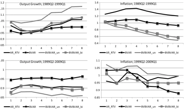
2-vintage values. The model we estimate is of the sort given by Eq.(34), where all of the observations come from the same (the latest) data vintage. This is in contrast to the approach embodied in the VB-VAR, which uses multiple vintages of data to estimate the model.Fig. 1presents the RMSFE ratios to the VAR(4) benchmark forh=
1, . . . ,
8 for both sub-periods and variables.The choice of the out-of-sample period is shown to affect the ranking between the performances of the bivariate and univariate BVB-VARs. In the earlier period (1989–99), the bivariate model improves the forecasts of output growth, but it does not do so in the later period. In contrast, the bivariate model yields superior inflation forecasts in the later period (1999–2009), but not when the forecast period consists of the 1990s. We also consider whether the modelling of data revisions has the same effect across the two periods; seeFig. 1. For output growth, the BVB-VAR clearly provides more accurate forecasts than the traditional BVAR for the second subsample. For inflation, the BVB-VAR is superior at all forecast horizons in the first subsample, and similarly in the second subsample, except at the longer horizons. In summary, we find some evidence of instability in the relative forecasting performances of the BVB-VAR specifications.
Table 2
Bayesian VB-VAR versus other forecasting models: RMSFE, recursive forecasting scheme. Forecasting vintages: 1989:Q2–2009:Q1.
yt+h AR_RTV VAR(4) BVAR(4) BVB-VAR_un BVB-VAR_bi VB-VAR_un VB-VAR_bi
Forecasting output growth
1 2.482 1.07 1.02 0.99 1.00 1.00 1.13 2 2.742 1.08 1.03 0.99 1.00 1.02 1.13 3 2.795 1.07 1.02 0.99 1.00 1.02 1.11 4 2.825 1.08 1.03 1.00 1.00 1.01 1.12 5 2.837 1.07 1.03 1.00 1.00 1.01 1.09 6 2.842 1.06 1.02 1.00 0.99 0.99 1.06 7 2.838 1.05 1.02 1.00 0.99 0.99 1.05 8 2.818 1.05 1.02 1.01 1.00 0.99 1.04 Forecasting inflation 1 0.921 0.94 0.97 0.98 0.95 1.02 1.00 2 1.023 0.90 0.94 0.88 0.85 1.07 1.04 3 1.143 0.85 0.89 0.83 0.81 1.05 1.01 4 1.243 0.84 0.86 0.80 0.77 1.03 0.97 5 1.321 0.88 0.85 0.77 0.76 1.00 1.03 6 1.427 0.88 0.84 0.74 0.73 1.01 1.01 7 1.537 0.90 0.83 0.71 0.71 1.00 0.98 8 1.599 0.89 0.81 0.67 0.68 0.99 0.92
Notes: The first column reports RMSFEs for the benchmark model, the AR_RTV. Subsequent columns give RMSFEs as ratios of the benchmark, where a value less than 1 indicates that the model in question has a smaller RMSFE than the benchmark. The BVAR(4) model is estimated in levels of the variables (all other models are estimated in growth rates) with the ‘sum of coefficients’ prior. The models are estimated using expanding windows of data.
Fig. 1. Consistency of relative forecasting performances.
5. Conclusions
In this paper we propose modelling and forecasting macroeconomic variables that are subject to revisions using a Bayesian vintage-based VAR. The vintage-based VAR models in the literature are typically univariate; that is, they model the relationships between different
maturities of data of a single variable. While such ap-proaches have shown promise in forecasting revisions of data for which initial estimates have been published, they are less successful at forecasting post-revision values of fu-ture observations. The use of a Bayesian approach allows us to build multivariate multiple-vintage models. In our em-pirical work, these models are estimated for output growth
Table 3
Bayesian VB-VAR versus other forecasting models, rolling forecasting scheme. Vintages at forecast origin: 1989:Q2–2009:Q1.
yt+h AR_RTV VAR(4) BVAR(4) BVB-VAR_un BVB-VAR_bi
Forecasting output growth
1 2.458 1.08 1.03 1.00 1.01 2 2.724 1.08 1.03 1.00 1.00 3 2.782 1.10 1.03 1.00 0.99 4 2.814 1.10 1.04 1.00 0.99 5 2.825 1.08 1.04 1.00 1.00 6 2.830 1.06 1.02 1.01 0.99 7 2.832 1.04 1.02 1.01 0.99 8 2.812 1.05 1.02 1.01 0.99 Forecasting inflation 1 0.861 0.99 1.01 1.04 1.00 2 0.956 0.96 0.99 0.93 0.89 3 1.049 0.90 0.96 0.90 0.86 4 1.120 0.90 0.93 0.89 0.83 5 1.167 0.93 0.93 0.88 0.83 6 1.253 0.93 0.92 0.85 0.81 7 1.332 0.95 0.92 0.84 0.80 8 1.368 0.94 0.91 0.81 0.76
Notes: See the notes toTable 2, except that the estimation uses rolling windows of data.
Table 4
Bayesian VB-VAR versus other forecasting models: variance, recursive forecasting scheme. Forecasting vintages 1989:Q2–2009:Q1.
yt+h AR_RTV VAR(4) BVAR(4) BVB-VAR_un BVB-VAR_bi VB-VAR_un VB-VAR_bi
Forecasting output growth
1 2.456 1.02 0.99 1.00 1.00 1.01 1.13 2 2.707 1.01 0.98 1.01 1.01 1.02 1.11 3 2.757 0.99 0.97 1.01 1.00 1.03 1.09 4 2.787 1.00 0.98 1.01 1.00 1.02 1.10 5 2.806 0.99 0.99 1.01 1.01 1.02 1.07 6 2.810 0.99 0.97 1.01 1.00 1.00 1.04 7 2.810 0.98 0.98 1.01 1.00 1.00 1.03 8 2.795 0.99 0.99 1.01 1.00 0.99 1.03 Forecasting inflation 1 0.872 0.99 1.02 1.04 1.01 1.06 1.05 2 0.925 0.99 1.03 0.97 0.94 1.14 1.13 3 1.003 0.95 1.00 0.94 0.91 1.12 1.13 4 1.048 0.97 1.00 0.95 0.89 1.11 1.12 5 1.074 1.02 1.00 0.95 0.92 1.07 1.23 6 1.124 1.02 1.00 0.93 0.89 1.09 1.22 7 1.180 1.04 1.00 0.92 0.89 1.10 1.19 8 1.184 1.03 1.01 0.90 0.87 1.10 1.13
Notes: Entries in the first column are the square root of the forecast error variance, computed as the square root of the difference between the MSFE and the squared average bias (which is the square of the average of the difference between actuals and forecasts). Subsequent columns are forecast error standard deviations as ratios of the benchmark, where a value less than 1 indicates that the model in question has a smaller variance than the benchmark. See also the notes toTable 2.
and inflation, and are shown to provide competitive fore-casts of the post-revision (or fully-revised) values of future inflation.
We show that the nature of data revisions suggests a prior for the Bayesian approach. Specifically, the prior captures the fact that data releases after the first few are likely to be efficient, in the sense of being largely unpre-dictable. This information is incorporated in a way thatde factoresults in more accurate forecasts than simply impos-ing sharp zero restrictions, as in the RV-VAR (compare the RV-VAR and BVB-VAR results inTable 1). This enhances the benefits of including other variables, but without a large penalty from increasing the parameter uncertainty.
We find that the VB-VAR, in conjunction with Bayesian estimation, delivers the most sizeable improvements for inflation forecasting. For the full 20-year out-of-sample pe-riod, the bivariate model is no better than the univariate model. However, for the more recent period (1999–2009), the bivariate VB-VAR is markedly better than the unviari-ate VB-VAR. We find that our implementation10 of the
Bayesian approach ofBańbura et al.(2010), which does not model multiple vintages, is far less successful for forecast-ing inflation than the VB-VAR.
10 Note that our implementation of their model is based only on output growth and inflation, whereas their framework allows for a large number of variables.
Acknowledgments
We would like to thank Fashid Vahid and two anony-mous referees of this journal for very useful comments and suggestions. Carriero and Galvão acknowledge support for this work from the Economics and Social Research Coun-cil [ES/K010611/1].
References
Aruoba, B., Diebold, F. X., Nalewaik, J., Schorfheide, F., & Song, D. (2013).Improving GDP measurement: A measurement-error perspec-tive. Mimeo: University of Pennsylvannia.
Bańbura, M., Giannone, D., & Reichlin, L.(2010). Large Bayesian vector autoregressions.Journal of Applied Econometrics,25(1), 71–92. Carriero, A. (2007).A Bayesian framework for the expectations hypothesis:
How to extract additional information from the term structure of interest rates. Working Papers 591, Queen Mary, University of London, School of Economics and Finance.http://ideas.repec.org/p/qmw/qmwecw/ wp591.html.
Carriero, A., Clark, T., & Marcellino, M.(2013). Bayesian VARs: specifica-tion choices and forecast accuracy.Journal of Applied Econometrics, in press.
Carriero, A., Kapetanios, G., & Marcellino, M.(2009). Forecasting exchange rates with a large Bayesian VAR.International Journal of Forecasting, 25(2), 400–417.
Carriero, A., Kapetanios, G., & Marcellino, M. (2012). Forecasting government bond yields with large Bayesian vector autoregressions. Journal of Banking and Finance,36(7), 2026–2047.
Chib, S.(1995). Marginal likelihood from the Gibbs output.Journal of the American Statistical Association,90(432), 1313–1321.
Clements, M. P., & Galvão, A. B.(2012a).Anticipating early data revisions to US output growth. Mimeo: University of Warwick and Queen Mary University of London.
Clements, M. P., & Galvão, A. B.(2012b). Improving real-time estimates of output gaps and inflation trends with multiple-vintage VAR models. Journal of Business and Economic Statistics,30(4), 554–562. Clements, M. P., & Galvão, A. B. (2013a). Forecasting with vector
autoregressive models of data vintages: US output growth and inflation.International Journal of Forecasting,29(4), 698–714. Clements, M. P., & Galvão, A. B.(2013b). Real-time forecasting of inflation
and output growth with autoregressive models in the presence of data revisions.Journal of Applied Econometrics,28, 458–477. Cunningham, A., Eklund, J., Jeffery, C., Kapetanios, G., & Labhard, V.(2012).
A state space approach to extracting the signal from uncertain data. Journal of Business and Economic Statistics,30, 173–180.
Doan, T., Litterman, R., & Sims, C. A.(1984). Forecasting and conditional projection using realistic prior distributions.Econometric Reviews,3, 1–100.
Fixler, D. J., & Grimm, B. T.(2005). Reliability of the NIPA estimates of U.S. economic activity.Survey of Current Business,85, 9–19.
Fixler, D. J., & Grimm, B. T.(2008). The reliability of the GDP and GDI estimates.Survey of Current Business,88, 16–32.
Garratt, A., Lee, K., Mise, E., & Shields, K.(2008). Real time representations of the output gap.Review of Economics and Statistics,90, 792–804. Garratt, A., Lee, K., Mise, E., & Shields, K.(2009). Real time representations
of the UK output gap in the presence of model uncertainty. International Journal of Forecasting,25, 81–102.
Geweke, J.(2005).Contemporary Bayesian econometrics and statistics. New Jersey: John Wiley & Sons, Wiley.
Giannone, D., Lenza, M., & Primiceri, G. E. (2012).Prior selection for vector autoregressions. CEPR Discussion Papers 8755, C.E.P.R. Discussion Papers.
Hecq, A., & Jacobs, J.P.A.M. (2009).On the VAR-VECM representation of real time data. Technical report. Mimeo: University of Maastricht, Department of Quantitative Economics.
Jacobs, J. P. A. M., Sarferaz, S., Sturm, J., & van Norden, S. (2013).Modelling multivariate data revisions.CIRANO—Scientific Publication N. 2013/44. Jacobs, J. P. A. M., & van Norden, S.(2011). Modeling data revisions: Measurement error and dynamics of ‘true’ values. Journal of Econometrics,161, 101–109.
Kadiyala, K. R., & Karlsson, S.(1997). Numerical methods for estimation and inference in Bayesian VAR-models.Journal of Applied Economet-rics,12(2), 99–132.
Kishor, N. K., & Koenig, E. F.(2012). VAR estimation and forecasting when data are subject to revision.Journal of Business and Economic Statistics, 30, 181–190.
Koenig, E. F., Dolmas, S., & Piger, J.(2003). The use and abuse of real-time data in economic forecasting.The Review of Economics and Statistics, 85(3), 618–628.
Koop, G.(2013). Forecasting with medium and large Bayesian VARs. Journal of Applied Econometrics,28, 177–203.
Landefeld, J. S., Seskin, E. P., & Fraumeni, B. M.(2008). Taking the pulse of the economy.Journal of Economic Perspectives,22, 193–216. Litterman, R.(1986). Forecasting with Bayesian vector autoregressions
-five years of experience.Journal of Business and Economic Statistics,4, 25–38.
Patterson, K. D.(1995). An integrated model of the data measurement and data generation processes with an application to consumers’ expenditure.Economic Journal,105, 54–76.
Patterson, K. D.(2003). Exploiting information in vintages of time-series data.International Journal of Forecasting,19, 177–197.
Schorfheide, F., & Song, D. (2013).Real-time forecasting with a mixed-frequency VAR. NBER working paper no. 19712.
Sims, C. A., & Zha, T.(1998). Bayesian methods for dynamic multivariate models.International Economic Review,39(4), 949–968.
Stark, T., & Croushore, D.(2002). Forecasting with a real-time data set for macroeconomists.Journal of Macroeconomics,24, 507–531. Stock, J. H., & Watson, M. W.(2003). Forecasting output and inflation: The
role of asset prices.Journal of Economic Literature,41, 788–829. Stock, J. H., & Watson, M. W.(2007). Why has U.S. inflation become harder
to forecast?Journal of Money, Credit and Banking,Supplement to Vol. 39, 3–33.
Stock, J. H., & Watson, M. W. (2009). Phillips curve inflation forecasts, understanding inflation and implications for monetary policy. Federal Reserve Bank of Boston.
Stock, J. H., & Watson, M. W. (2010).Modelling inflation after the crisis, NBER Working Paper Series 16488.
Theil, H., & Goldberger, A. S. (1961). On pure and mixed statistical estimation in economics.International Economic Review,2(1), 65–78.
Andrea Carrierois Professor of Economics at the School of Economics and Finance, Queen Mary University of London.
Michael P. Clements is Professor of Econometrics at ICMA Centre, University of Reading, and associate member of the Institute for New Economic Thinking, Oxford Martin School, University of Oxford.
Ana Beatriz Galvãois Associate Professor of Economic Modelling and Forecasting at Warwick Business School, University of Warwick.