3
Detecting spatial and temporal house price diffusion
in the Netherlands: A Bayesian network approach
Published as: Teye, A.L., Ahelegbey, D. F. (2017). “Detecting spatial and temporal house price diffusion in the Netherlands: A Bayesian network approach”. Regional Science and Urban Economics, Volume 65(4), pp. 56-64.
Abstract
Following the 2007-08 Global Financial Crisis, there have been a growing research interest on the spatial interrelationships between house prices in many countries. This paper examines the spatio-temporal relationship between house prices in the twelve provinces of the Netherlands using a recently proposed econometric modelling technique called Bayesian graphical vector autoregression (BG-VAR). This network approach enables a data driven identification of the most dominant provinces where house price shocks may largely diffuse through the housing market and it is suitable for analysing the complex spatial interactions between house prices. Using temporal house price volatilities for owner-occupied dwellings, the results show evidence of house price diffusion pattern in distinct sub-periods from different provincial housing sub-markets in the Netherlands. We observed particularly prior to the crisis, diffusion of temporal house price volatilities from Noord-Holland.
Keywords:Graphical models, House price diffusion, Spatial dependence, Spillover effect
...
§ 3.1
Introduction
...
The collapse of house prices during the 2007-08 Global Financial Crisis (GFC) slowed down economic growth in many countries. After the GFC, researchers and governments alike have been seeking to understand the dynamics of house price development in order to resuscitate the stagnating housing market and the general economy. This has consequently led to a new research agenda that specifically seeks insights into spatial interactions and diffusion between the regional housing markets. House prices vary over space and time, but developments of house prices across regions may not be entirely independent of each other. As explained byGong et al.(2016b), there are significant variations in regional house prices. However, house prices interrelate spatially over time, and it is paramount for governments to understand these interrelationships so as to formulate policies to regulate the overall functioning of the housing market.
Spatial interrelationships between regional house prices may take the form of a long-run convergence or a temporal diffusion mechanism. Long-run convergent
property markets equilibrate and remain integrated over a long period of time (Holmes and Grimes,2008;Cook,2005;Cotter et al.,2011). Temporal house price diffusion is also sometimes known in the literature as ripple or spillover effect (seeMeen,1999). This market phenomenon depicts the situation where house price shocks in one region is believed to propagate to house prices in other regions with a transitory or permanent effect (Balcilar et al.,2013;Canarella et al.,2012;Pollakowski and Ray,1997). Empirical evidence in support of this temporal house price diffusion mechanism exists in the context of the US (Canarella et al.,2012;Holly et al.,2010;Pollakowski and Ray,
1997) and the UK (Meen,1999,1996;Holly et al.,2011). More recent results from China and other developing countries also lend support to the house price diffusion hypothesis (seeGong et al.,2016b;Lee and Chien,2011;Nanda and Yeh,2014;
Balcilar et al.,2013). However, in most of these previous studies, the hypothesis is tested for a lead-lag relationship where it is assumeda priorithat the diffusion will start from some economically “superior region”.
In this paper, we shed light on the spatial and temporal house price diffusion in the case of the Netherlands. The focus is specifically as follows. First, we investigate if there is a spatial dependence of temporal house price volatilities and a diffusion pattern between provinces in the Netherlands. Secondly, we are interested in identifying from the data the provinces which may serve as the dominant sources of house price shocks. Lastly, we investigate if these spatio-temporal relationships vary over time.
We employ a graphical network approach for studying these spatio-temporal house price dynamics. Graphical modelling is a class of multivariate analysis that uses graphs consisting of nodes and edges to study the interaction and path dependence between variables. The nodes of this graph represent the variables while the edges (or links) denote their interactions and dependence structure (seeLauritzen,1996;Eichler,
2007). The graphical modelling approach has become popular as a more natural way to discover hidden and complex interactions among multiple variables. It is applied mostly in the study of contagion and systemic risk analysis in the financial sector where there is complicated and non-linear relationships between variables (seeAhelegbey,
2016, for a more comprehensive review). Like most financial variables, one indeed expects a complex interrelationships between regional house prices which can easily be handled by the graphical network approach.
This paper specifically adopts the graphical method recently proposed byAhelegbey et al.(2016a) called the Bayesian Graphical Vector Autoregression (BG-VAR). The BG-VAR is a data-driven approach where the directed edges of the network represent causal relationships. The empirical application in this paper uses quarterly data (1995:Q1 - 2016:Q1) on temporal house price volatilities for second-hand
owner-occupied dwellings from the twelve provinces of the Netherlands. The results establish a temporal dependence and diffusion dynamics existing between the provincial housing markets. These spatial relationships, however, vary over time in terms of the degree of dependence and the centrally dominant sub-markets. In particular, between 1995Q1 and 2005Q2, Noord-Holland was most predominant, whereas the central regional housing market in the period 2005Q3–2016Q1 was Drenthe.
We organised the remaining sections of the paper as follows. A brief overview of the related literature is provided in Section 3.2. Section 3.3 describes the BG-VAR model.
The description of the data is presented in Section 3.4 while Section 3.5 discusses the empirical results. The entire paper is concluded in Section 3.6.
...
§ 3.2
Extant literature
...
Many scholars have been working on the spatio-temporal house price diffusion or the so-called ripple effect and a vast literature now exist. An extensive review of the literature is provided byBalcilar et al.(2013) and most recently byNanda and Yeh
(2014) andGong et al.(2016b). We only provide a brief summary here. The study of this ripple effect hypothesis actually began from the UK when English researchers observed that house prices rise, during an upswing, first from the South-East (mostly London) and then spread out to other parts of the country (Giussani and
Hadjimatheou,1991;Meen,1996,1999). According toPollakowski and Ray(1997) house price diffusion will not necessarily occur between neighbouring housing markets, but may require some form of economic interrelationship.Meen(1999) likewise shared the view ofPollakowski and Ray(1997), and noted that spatial dependence may not be necessary for explaining the ripple effect.Meen(1999) then suggested four probable mechanisms through which rising house prices from one region may later manifest in other parts of the UK. These channels according to the author include: migration, equity transfer, spatial arbitrage and spatial patterns in house price determinants. As also noted later byCanarella et al.(2012), migration particularly may lead to house price ripple effect if households relocate in response to changes in the spatial distribution in house prices.
Meen(1999) also provided an empirical framework for testing the ripple effect by assuming that regional house prices will react to shocks at different rates. The author’s approach was equivalent to testing the stationarity of the regional to national house price ratios. AlthoughMeen(1999) was unsuccessful in confirming the ripple effect with the Augmented Dickey-Fuller test, the author’s empirical framework became the basis for other scholars who later found empirical evidence using more sophisticated stationarity test procedures.Cook(2003), for instance adopted the Threshold Autoregressive (TAR) and Momentum Threshold Autoregressive (MTAR) test
procedures whileHolmes and Grimes(2008) used a combination of unit root test and Principal Component Analysis (PCA) to confirm the spillover effect in the UK.Canarella et al.(2012) similarly studied the house price diffusion effect in the US by using a combination of the Generalised Least Squares (GLS) version of the Dickey-Fuller, non-linear unit root tests and other test procedures that control for structural breaks.
Balcilar et al.(2013) also adopted a Bayesian and non-linear unit root tests, with and without structural breaks to investigate the ripple effect in the South African housing market. The Panel Seemingly Unrelated Regressions Augmented Dickey-Fuller (SURADF) has equally been employed by other scholars (e.g.Lee and Chien,2011;
Holmes,2007).
Recently, tremendous effort, relying on the advances in the econometric literature, has also been channelled into refining the methodology for testing the ripple effect hypothesis beside the “Meen framework”.Holly et al.(2011), for example proposed a dynamic modelling approach where they allowed shocks from the dominant region to propagate to other regions and then echo back. The authors found support for the ripple effect using this approach for the UK with London as the dominant region.Gong
et al.(2016b) adopted similar method in their study of ripple effect for 10 regions in the Pan-Pearl river of China.Nanda and Yeh(2014), in a related study also suggested using a dynamic panel-spatial model. Some studies equally advocated formulating a Spatial Vector Autoregressive (SPVAR) model and subsequently testing for Granger Causality (GC) and/or performing Impulse Response Analysis (IRA) to examine the ripple effect hypothesis.Brady(2014), for example captured the spatial diffusion between regional housing prices in the US with impulse response functions estimated from a Spatial Autoregressive (SAR) model.
Pinkse and Slade(2010) as well asGibbons and Overman(2012), however, argued that the SAR model and many other spatial models (seeLeSage and Pace,2009;Florax and Folmer,1992;Dubin,1992) may suffer generally from mis-specification because the spatial weighting matrices which are central to those models are constructed in an ad-hoc manner. Other authors entirely avoid constructing the spatial weighting matrix by estimating traditional VAR to perform GC and IRA. For instance,Vansteenkiste and Hiebert(2011) adopted a global VAR model and IRA to study the house price spillover effects across countries in the euro area.Gupta and Miller(2012a), similarly
formulated traditional VAR model after which they tested for GC and performed IRA to verify the spatial diffusion phenomenon between Los Angeles, Las Vegas, and Phoenix in the US.
The VAR based models, similarly suffer from mis-specification or over-parametrisation, which may render the impulse response function and GC test inaccurate (seeKoop and Korobilis,2010;Vega and Elhorst,2013;George et al.,2008). To eliminate the problem of mis-specification and over-parametrisation,Ahelegbey et al.(2016a) recently proposed the Bayesian graphical network vector autoregressive (BG-VAR) method which provides a better approach to specify and estimate a parsimonious VAR model. The novelty of the BG-VAR is that, we can identify the temporal dependence structure between the variables without having to estimate the structural (VAR) parameters.
In addition, the method could be used to identify the direction of dependence between the variables and it is somewhat related to the concept of GC. The GC, however adopts a pairwise (or conditional pairwise) analysis to identify the dependence patterns without accounting for the structural uncertainties. On the other hand, the BG-VAR employs a Bayesian technique which incorporates necessary prior information to explore the structure and to apply model averaging.Ahelegbey(2016) provided empirical evidence that support the superior efficiency of the BG-VAR over the GC in producing
dependence patterns that are more suitable for capturing complex interdependencies. Investigating the dependence structure between multiple time series with the BG-VAR model is generally more convenient for researchers and policy makers to understand directional or causal relationships.
...
§ 3.3
The Bayesian graphical vector autoregressive (BG-VAR) model
...
This section presents the formulation of the BG-VAR model adopted in this paper. Assume for a moment that temporal house price volatilities in one region is a result of earlier shock to house prices in other regions. We can formulate a vector autoregressive process of orderp(VAR(p)) to capture these interdependencies. As mentioned earlier,
some authors study the spatial and temporal house price dynamics by testing for Granger causality (GC) and performing IRA from this underlying VAR model. LetYtdenote the vector of house price volatilities at the timetfromnregions which
are demeaned. We can write the VAR(p) process forYtfollowing the equation Yt=
p
∑
i=1
BiYt−i+ut=BXt+ut, ut∼ N(0,Σu) (3.1)
wheret = p + 1, . . . , T;pis the maximum lag order to be chosen and
Xt = (Yt′−1, . . . , Yt′−p)′isnp×1stacked matrices of the lagged regional house price
volatilities.B = (B1, . . . , Bp), whereBi,1≤i≤pis ann×nmatrix of coefficients,
which determine the dependence of the house price volatilities on their lags. The set of equations in (3.1) captures the structure of the interactions between the regional house price volatilities andAhelegbey et al.(2016a) showed that the temporal dependencies between them could be inferred fromB. For example, when the volatility of house prices in one region depends only on a subset but not on earlier shock to house prices in all the regions, there are components ofBthat become zero. In general,Bijmeasures the anticipated effect of changes in thej-th predictor (Xj,t)
on the house price development in thei-th region (Yi,t).
Ahelegbey et al.(2016a) demonstrated that the VAR model (3.1) can be
operationalised as a graphical model using the relationB = (G◦Φ), whereGis a binary (0/1) matrix,Φis a coefficients matrix, both of dimensionn×np, and(◦)is the element-by-element product. The elements ofGrepresent the presence or absence of an edge (interaction) between volatility of house prices in pairs of regions. A
one-to-one correspondence betweenBandΦconditional onGcan be identified. That is,Bij= Φij̸= 0, ifGij= 1; andBij= 0, ifGij= 0.
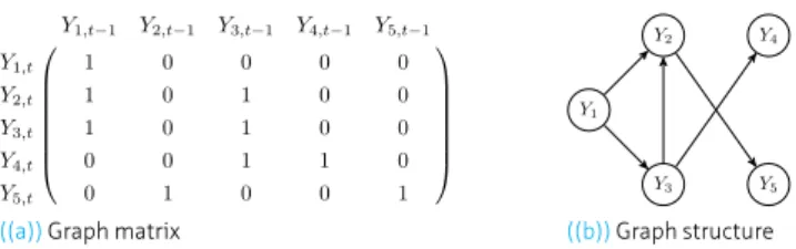
As an example, consider an arbitrary five-dimensional VAR(1) with coefficients matrix
B= β11 0 0 0 0 β21 0 β23 0 0 β31 0 β33 0 0 0 0 β43 β44 0 0 β52 0 0 β55 (3.2)
where the non-zero elements ofBare real numbers. The network that depicts the temporal dependence among the variables associated with (3.2) can be visualised in Figure3.1. The nodes of this network are specifically the five variables:Y1t, Y2t, Y3t, Y4t
andY5t. Sinceβ21 ̸= 0,Y1,t−1has a significant impact onY2,t. This also means that an
edge exists betweenY1andY2which is denoted asY1 →Y2. The edges of the network indicate the lagged dependencies between the variables without self lag effects, which are the indirect effects.
Elhorst(2014) andLeSage and Pace(2009) discussed the direct and the indirect (or spillover) effects between spatial variables. Figure3.1shows that the two effects may be easily distinguished with the BG-VAR approach. The direct effect are represented in the diagonal of the graph matrix G, while its off-diagonals describe the indirect interactions depicted by the Figure3.1(b). For the diffusion dynamics, it suffices to estimate only the network structure captured byG. LetDt = (Xt′, Yt′)′be ad×1
Y1,t−1 Y2,t−1 Y3,t−1 Y4,t−1 Y5,t−1 Y1,t 1 0 0 0 0 Y2,t 1 0 1 0 0 Y3,t 1 0 1 0 0 Y4,t 0 0 1 1 0 Y5,t 0 1 0 0 1
((a))Graph matrix
Y2 Y1 Y3 Y4 Y5 ((b))Graph structure
FIGURE 3.1 Network matrix and diagram associated with the temporal dependence in the five-dimensional VAR(1) process in (3.2).
vector, whered=n+npand assumeDt ∼ N(0,Ω−1), whereΩis ad×dprecision
matrix. The joint distribution for all the variables inDtcan be summarised with a
graphical model and represented by the pair(G,Ω) ∈ (G ×Θ). Here,Gis a directed acyclic graph (DAG) of the relationships among the variables inDt,Ωconsists of the
VAR model parameters,GandΘare the graph and parameter space respectively. The triple (Ω,Σu, B)are mathematical related. SupposeXt ∼ N(0,Σxx)and
Yt|Xt∼ N(BXt,Σu),BandΣucan be obtained from the covariance matrix ofDt(i.e.
Σ = Ω−1) by
B= ΣyxΣ−xx1, Σu= Σyy−ΣyxΣ−xx1Σxy (3.3)
whereΣyxisn×npcovariances betweenYtandXt,Σxxisnp×npcovariances among XtandΣyyisn×ncovariances amongYt. GivenB,ΣuandΣxx,Ωcan equally be
obtained using the well-known Sherman-Morrison-Woodbury formula (Woodbury,
1950), Ω = Σ−1= ( Σ−xx1+B′Σ− 1 u B −B′Σ− 1 u −Σ−1 u B Σ−u1 ) , where Σ = ( Σxx Σxy Σyx Σyy ) (3.4) By definingB = (G◦Φ), equation (3.4) shows howΩrelates toGthroughB. The specification of the BG-VAR model is completed with the choice of a hierarchical prior on the lag orderp, the graph structureGand the parameterΩ.
We now focus on the estimation procedure for the graph structure (G) associated with the temporal dependence between the regional house prices. In the Bayesian framework, the joint prior distribution of (p, G,Ω) is given by
P r(p, G,Ω) =P r(p)P r(G|p)P r(Ω|p, G). It is important to first select the optimal lag order for the VAR model. FollowingAhelegbey et al.(2016b), we choosepin the range 0 < pmin < pmax < ∞, for some lower boundpminand upper boundpmax. More specifically, we assumepfollows a discrete uniform prior on{pmin, . . . , pmax}with a distribution
P r(p) = 1
pmax−pmin+ 1
(3.5) Since we seek to estimate the regional market that is central in the spread of house price volatility from the data, it is more reasonable to assume a priori that any region is equally likely to play this role. This implies that the graph structure can be represented
as a product of local sub-graphs of each equation of the model and may be written as P r(G|p) = n ∏ i=1 P r(πi|p) (3.6)
whereπi={j= 1, . . . , np:Gij= 1}is the set of price volatilities of thei-th equation
predictors.
We formulate in what follows, the standard techniques for estimatingGalso described byAhelegbey et al.(2016a,b). We assume for each edgeGij, an independent Bernoulli
trial with conditional prior probability
P r(πi|p, γ) =γ|πi|(1−γ)np−|πi| (3.7)
where|πi|is the cardinality ofπiandγ ∈ (0,1)is the Bernoulli parameter. We use
a uniform graph prior by choosingγ = 0.5so thatP r(πi|p, γ = 0.5) = 2−npand P r(G|p)∝1.
Following standard Bayesian paradigm, we also assume thatΩconditional onpand a complete graphGis Wishart distributed,Ω∼ W(ν, S−1), with density
P r(Ω|p, G) = 1 Kd(ν, S) |Ω|(ν−d2−1)exp { −1 2⟨Ω, S⟩ } (3.8) where⟨A, B⟩=tr(A′B)is the trace inner product,νis the degree of freedom,Sis the prior sum of squared matrix andKd(ν, S)is the normalizing constant. The likelihood
of a random sampleD= (D1, . . . , DT)is multivariate Gaussian with density P r(D|p,Ω, G) = (2π)−12dT|Ω| 1 2Texp { −1 2⟨Ω,Sˆ⟩ } (3.9) whereSˆ=∑Tt=1DtDt′is ad×dsample sum of squared matrix.
Given thatGis unknown, a standard Bayesian approach for determining the graph structure is to integrate outΩfrom (3.9) with respect to its prior given by
P r(D|p, G) =
∫
P r(D|p,Ω, G)P r(Ω|p, G)dΩ =Kd(ν+T, S+ ˆS) (2π)12dTKd(ν, S)
(3.10) whereS + ˆSis the posterior sum of squared matrix. The expression (3.10) is the marginal likelihood function expressed as ratio of the normalising constants of the Wishart posterior and prior. Following standard application, the marginal likelihood factorises into the product of local terms, each involvingYi,tand its set of selected
predictors,Xπi,t, given by P r(D|p, G) = n ∏ i=1 P r(D|p, Gi,πi) = n ∏ i=1 P r(D(i,πi)|p, G) P r(D(πi)|p, G) (3.11) whereD(i,πi)andD(πi)are sub-matrices ofDconsisting of(Y
i,t, Xπi,t)andXπi,t respectively. Letwi ∈({i} ∪πi). The closed-form expression for the left-hand side of
(3.11) is given by P r(Dwi|p, G) = π −1 2T|wi|ν12ν|wi| (ν+T)12(ν+T)|wi| |Σwi|12ν |Σ¯ wi| 1 2(ν+T) |∏wi| s=1 Γ(ν+T+12 −s) Γ(ν+12−s) (3.12) where|wi|is the cardinality ofwi,Σwiand
¯
Σwiare the prior and posterior covariance matrices ofDwi.
Again, we follow standard practice and setΣwi = I|wi|, whereI|wi|is a
|wi|-dimensional identity matrix.1By definition, (3.12) consists of a component that is
independent ofΣ¯w
i. We can reduce the computational time by expressing this independent component as a functionQν(|wi|, p, T)given by
Qν(|wi|, p, T) = π−12T|wi|ν12ν|wi| (ν+T)12(ν+T)|wi| |∏wi| s=1 Γ(ν+T+12 −s) Γ(ν+12−s) (3.13)
Since for each equation, we havenpnumber of explanatory variables,|wi|will be
bounded below by1and above bynp+ 1. Thus, we can setν=np+ 2. Givenν,Tand
p, Qν(|wi|, p, T)does not directly depend on the variables inwibut on
|wi| ∈ {1, . . . , np+ 1}. Hence, (3.12) may be expressed as P r(Dwi|p, G) =Q
ν(|wi|, p, T) |Σ¯wi| −1
2(ν+T) (3.14)
The posterior covariance matrix ofDis also given by ¯ Σ = 1 ν+T ( νId+ T ∑ t=1 DtD′t ) (3.15) Thus,Σ¯w
iin (3.14) can be obtained as a sub-matrix ofΣ¯which corresponds to the elements inwi. Pre-computingΣ¯andQν(|wi|, p, T)for|wi|givenν,Tandp, before
sampling the network matrix reduces the computational complexity and makes the algorithm efficient. The details of sampling the network structure is provided in the
Appendix to Chapter 3.
...
§ 3.4
Description of data
...
This section gives a brief background to the regional housing market in the Netherlands and describes the data. The spatial units for our analysis include the twelve official Dutch provinces.2These are, namely Drenthe (DR), Flevoland (FL), Friesland (FR), Gelderland (GE), Groningen (GR), Limburg (LI), Noord-Brabant (NB), Noord-Holland (NH), Overijssel (OV), Zuid-Holland (ZH), Utrecht (UT) and Zeeland (ZE) (see map in Figure3.2). According to Statistic Netherlands (CBS), Zuid-Holland is the largest in terms of GDP (141.758 billion Euros in 2014), followed by Noord-Holland (133.358
1 For anyn×nidentity matrixA, we have|A|= 1. 2 In this paper, we use region and province interchangeably.
FIGURE 3.2 Map of the twelve provinces of the Netherlands.
Source:d-maps.com
billion Euros in 2014). Zeeland is the smallest with estimated GDP of 11.429 billion Euros in 2014. The capital Amsterdam is hosted by Noord-Holland while the
government seat (The Hague) is located in Zuid-Holland. The extant literature suggest a higher tendency of house price shocks to diffuse from some “mega economic districts” to peripheral regions (seeGong et al.,2016b;Holly et al.,2011). Thus, our initial expectation is that Noord-Holland or Zuid-Holland may be central in the house price diffusion mechanism in the Netherlands within certain periods.
We use quarterly house price indexes spanning the period 1995Q1 to 2016Q1 for second-hand owner-occupied dwellings in this paper. The data is obtained from Statistic Netherlands (CBS). CBS is the Dutch official agency which publishes statistics on housing and other sectors of the economy. The indexes are constructed adopting the sale price appraisal ratio (SPAR) method (seede Haan et al.,2009). By using official annual appraised values for the dwellings and chaining the ratios, CBS adjusts for appraisal bias in the SPAR index but is unable to control for quality changes. Given available house transaction data, CBS’ SPAR index is the most reliable in the Netherlands (De Vries et al.,2009).
A simple plot of the house price indexes (Figure3.3) shows a common trend in the growth of house prices in all the twelve regional markets before and after the GFC. The periods prior to 2009 show a relatively faster house price appreciation which may be attributed to many factors. For instance, the Dutch government promoted home ownership forcefully during those periods with the National Mortgage Guarantee scheme and through an income tax structure that offered generous rebates on the
Time/Quarter Inde x 1995 2000 2005 2010 2015 40 60 80 100 DR FL FR GE GR LI NB NH OV UT ZE ZH
FIGURE 3.3 Dutch regional house price indexes.
Note:DR= Drenthe,F L= Flevoland,F R= Friesland,GE= Gelderland,GR= Groningen,LI= Limburg,N B
= Noord-Brabant,N H= Noord-Holland,OV= Overijssel,U T= Utrecht,ZE= Zeeland,ZH= Zuid-Holland. Source:Statistics Netherlands.
mortgage interest rates (see,Toussaint and Elsinga,2007;Boelhouwer et al.,2004;
Elsinga,2003;Boelhouwer,2002). These incentive packages generally made it cheaper for individual households to purchase their own dwellings, which consequently led to increase in demand and rise in house prices before the crisis.
As in other countries, financial institutions in the Netherlands were also hit by the 2007-08 GFC. The impact of the crisis on house prices however started in the last quarter of 2008 as seen in Figure3.3. Following the GFC, average house prices in the Netherlands declined by almost 25% between 2009 and 2013.Teulings(2014), attributed the collapse in the Dutch property values with the higher unemployment and redundancy rates during the meltdown. Other scholars however blamed the collapse on the Dutch financial institutions who tightened up mortgage accessibility and impeded new home buyers from the market (Elsinga et al.,2016;Boelhouwer,
2014;Bardhan et al.,2011). Since the beginning of 2014, there has been gradual recovery of Dutch house prices, somewhat faster in Zuid-Holland and Noord-Holland. In this paper, we study the temporal diffusion pattern of house price volatilities in the Netherlands. We followMartens and Van Dijk(2007) to define the house price volatilities for each region as the squared returns given by
SRt= [100(logIt−logIt−1)]2 (3.16)
whereItis the house price index at the timet. Figure3.4summarises the temporal
regional house price volatilities. It shows that house prices were more volatile in most regions from 1995 until the early 2000s, and gradually decline afterwards.
Time/Quarter Squared Retur ns 1995 2000 2005 2010 2015 0 10 20 30 40 DR FL FR GE GR LI NB NH OV UT ZE ZH
FIGURE 3.4 Regional house price volatilities.
...
§ 3.5
Spatio-temporal house price dynamics
...
We estimate the temporal dependencies from the network structure described in Section 3.3 using the (demeaned) regional house price volatilities. We set the
minimum and maximum lag order top= 1andp= 4respectively. The estimation first follow a twenty-quarter rolling window and the result is summarised with the network density to examine the extent of interdependencies between the regional house prices over time. The network density is a simple aggregate index for the degree of
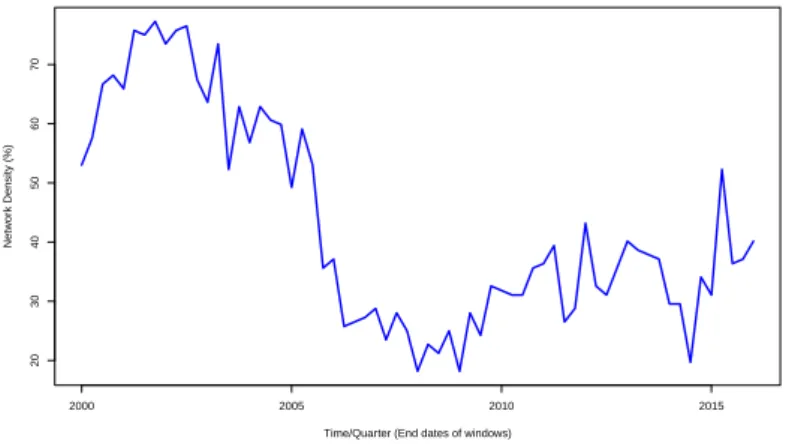
interdependence. It is defined for each estimation window as the percentage of the regions whose temporal house price volatilities are dependent on earlier price movements in other regions. More specifically, the network density is the number of identified edges in the network divided by the total possible edges. Fornnumber of regions or variables, there aren(n−1)possible edges indicating the indirect effects. Figure3.5presents the network density associated with the temporal regional house price volatility interdependencies. The average network density over the study period is about 43%, which gives evidence of temporal interdependence and diffusion between the regional house price volatilities. Figure3.5also shows that the degree of
interdependence varies over time. It was higher particularly between 1995 and 2005, then began to decrease until 2008, after which it has been on the rise again.
The above sub-periods somewhat coincide with recognisable stages in the development of house prices in the Netherlands. It is recognised by most Dutch researchers that the period 1995–2005 is one during which house prices increased legitimately because of the rise in household disposable income and government stimulation of the housing market (De Vries,2010;Toussaint and Elsinga,2007;
Boelhouwer et al.,2004;Boelhouwer,2002). On the other hand, some analysts argued that the Dutch house price development from 2005–2008 was mostly due to
over-valuation and speculative investment activities which also precipitated the crisis that started in the last quarter of 2008 (Xu-Doeve,2010;Aalbers,2009a,b).
Time/Quarter (End dates of windows) Netw or k Density (%) 2000 2005 2010 2015 20 30 40 50 60 70
FIGURE 3.5 Network density estimated with rolling window over the period 1995Q2 – 2016Q1.
§ 3.5.1 Sub-period dynamics
...
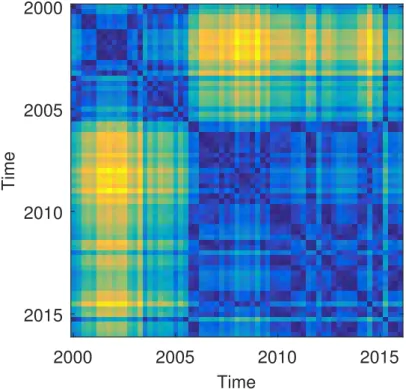
To ascertain if the central regions in the house price diffusion dynamics vary with time, we study in details the network structure within sub-periods. It is appropriate to identify if there are structural shifts in the network density and delineate the sub-periods along them. A simple recurrent plot (Marwan et al.,2007) in Figure3.6
shows a significant period of structural change in the network density, occurring between 2005 and 2006.3Using the sequential method ofBai and Perron(2003,
1998), we also test for the structural shift and the break date. The sequential test assumes no knowledge of the break date but requires that a model for the series and maximum likely breaks are specified. FollowingBrady(2014), we model the series for the network density as an AR(1) process. We allow up to 3 breaks, however the BIC suggests only one significant structural shift, occurring at 2005Q2. This confirms the recurrent plot also suggesting one structural shift.
We re-estimate the network structure for the two sub-periods: 1995Q1–2005Q2 and 2005Q3–2016Q1. The summary statistics and optimal lag order associated with the network structure for each specific sub-period are presented in Tables3.1and3.2. The average path length, for example, represents the average graph-distance between all pair of nodes, where interconnected nodes have graph distance of 1. In general, the higher the graph distance the slower it takes house price shocks in one region to cascade systemically. Table3.1also indicates the total links and average degree which are important for the network analysis.
The interest here is to identify the regions with temporal house price volatilities that are predominately interdependent and their specific direction of interconnection with the others. These regions are interesting because they play important role in the transmission of house price shocks. In the network terminology, these regions are the
3 A recurrence plot is a way to visualise and study the dynamics of phase space by a two- dimensional plot (Marwan et al.,2007).
2000
2005
2010
2015
Time
2000
2005
2010
2015
Time
FIGURE 3.6 Recurrent plot indicating the patterns in the network density over time.
hub-centralities (see,Benzi et al.,2013). The network structures for the two sub-periods are presented in Figure3.7. The figure shows the explicit nature and degree to which the regional house price volatilities are temporarily dependent on one another. For example, it indicates a direct temporal dependence of house price volatilities in Nord-Brabant on Noord-Holland between 1995Q1 and 2005Q2 but not during the period 2005Q3–2016Q1. As with Figure3.5, Figure3.7similarly reveals that there is heavier dependency between the regional house prices before 2005 than it was afterwards. Again, this may indicate the shift in the developments of Dutch house prices.
TABLE 3.1 The network statistics for the sub-period graphs.
Edges/Links Density Average Degree Average Path Length
1995Q1–2005Q2 94 0.71 15.67 1.29
2005Q3–2016Q1 39 0.30 6.50 1.73
TABLE 3.2 Equation-specific lag order of each equation for the sub-periods.
Period DR FL FR GE GR LI NB NH OV UT ZE ZH
1995Q1–2005Q2 3 2 1 2 4 2 2 2 2 2 1 2
FL FR GE GR LI NB NH OV UT ZE ZH DR ((a))1995Q1 – 2005Q2 GR NB OV UT ZH DR LI NH FR GE FL ZE ((b))2005Q3 – 2016Q1
FIGURE 3.7 Network diagrams showing the temporal dependence between house price volatilities of the 12 Dutch regional markets during sub-periods.
Note:The sizes of the nodes are proportional to the degrees (number of other regions to which the specified region at the node is connected to).
To determine the hub-centrality, we use the Katz measure (Katz,1953). The Katz measure scores the centrality of a region by considering its direct and indirect
interdependences with other regions. Table3.3presents the centralities and the ranks associated with the network structure in Figure3.7for each region. The table indicates Noord-Holland as the most central during the period 1995Q1–2015Q2, while Drenthe ranks the most central for the sub-period 2005Q3–2016Q1. As one of the largest economic regions (mainly due to influence of the national capital, Amsterdam), it is not surprising that Noord-Holland is central in the temporal house price diffusion pattern. Earlier studies (e.g.Holly et al.,2011;Giussani and Hadjimatheou,1991) similarly found that house prices diffusion in the UK exists from the economic hub, London. On the other hand, the result of Table3.3shows that economically smaller regions such as Drenthe may equally be pivotal in diffusion of house prices during certain periods. Although it is unclear why smaller regions will be that central, suburbanisation and recent trend of urban to rural migration of certain class of people in the Netherlands, majority who are seniors, may play some role (seeDe Jong et al.,2016;Accetturo et al.,
2014;Van Ommeren et al.,1999).
The network distance in Table3.3may be used to further examine the diffusion dynamics of temporal house price volatilities from the central regions. The network distance is by definition the length of the shortest path between two nodes in the network. A network distance of 1 denotes a direct interdependence, while a distance of 2 indicates the interdependence between two nodes that is mediated by another node. In tandem with this description, the results of Table3.3may be interpreted to mean that, temporal house price volatility from Noord-Holland in the period
1995Q1–2005Q2 had a direct causal relationship with the volatility of house prices in the other regions, except Friesland and Zeeland where this was mediated. Similarly, we find that temporal causal relationships exist between house price volatility in Drenthe and the rest of the regions during the period 2005Q3–2016Q1, except Zeeland for which this was mediated.
TABLE 3.3 Hub centrality, rank and distance associated with the network for the sub-periods.
1995Q1 – 2005Q2 2005Q3 – 2016Q1
Centrality Rank Distance Centrality Rank Distance
Drenthe 54.55 12 1 23.65 1 0 Flevoland 212.72 3 1 1.00 12 1 Friesland 139.46 9 2 1.78 9 1 Gelderland 136.25 10 1 1.66 10 1 Groningen 163.18 6 1 17.59 2 1 Limburg 179.52 5 1 11.68 3 1 Noord-Brabant 212.98 2 1 1.80 8 1 Noord-Holland 228.85 1 0 2.96 6 1 Overijssel 122.96 11 1 5.25 5 1 Utrecht 142.55 8 1 7.18 4 1 Zeeland 151.88 7 2 1.00 11 2 Zuid-Holland 207.51 4 1 1.80 7 1
The bold values indicate the hubs.
...
§ 3.6
Summary and concluding remarks
...
In an effort to revive the housing markets that have collapsed in many countries following the 2007–2008 Global Financial Crisis (GFC), there is an ongoing research agenda that seeks understanding into the spatio-temporal dynamics of house prices. This paper makes three main contributions to this new research area. Firstly, the paper studied the spatio-temporal house price dynamics in the unique context of the Netherlands, which is first of its kind. Here, the paper specifically asked if there is temporal spatial dependence of house prices in the Netherlands. It then investigated the diffusion pattern and identified the specific regions where temporal house price volatilities are likely to spread.
For the second contribution, the paper demonstrated the usefulness of graphical and network techniques in analysing the spatio-temporal house price dynamics.
Particularly, the paper adopted the newly proposed Bayesian graphical vector autoregression (BG-VAR) model which is in general more efficient in identifying dependence patterns between multiple variables than the traditional concept of Granger Causality (seeAhelegbey et al.,2016a). As a third contribution, the paper proposed a simple data driven techniques to identify the regional housing sub-market where diffusion of temporal house price volatilities may predominately start. This approach deviates from previous studies which assumeda priorisome “bigger cities” as most central in investigating the house price diffusion process (e.g.Holly et al.,
2011). The potential selection bias is avoided in our approach because the central region can be easily inferred from the network using statistical measures for the centrality.
In the empirical analysis, the paper used temporal volatilities constructed from quarterly house price indexes for owner-occupied dwelling between 1995Q1 and 2016Q1. The results, based on the BG-VAR model and various network statistics, support a temporal dependence and diffusion of house prices in the Netherlands. We also observed that the degree of temporal interdependence varies over time. Especially, we found that the Dutch regional house prices were highly interdependent between 1995 and 2005. After 2005, the degree of interdependence weakened until 2008 and again increased from 2008 to 2016 (Figure3.5). We performed formal empirical break tests, which suggest that a structural shift in the temporal dependence actually exists
at 2005Q2 (see Figure3.6). The break may reflect some experts’ believe of Dutch housing investments shifting to more speculative activities which also precipitated the severe decline of house prices after 2008 (seeXu-Doeve,2010;Aalbers,2009a). Studying in more detail the resulting sub-periods 1995Q1–2005Q2 and
2005Q3–2016Q1, we identified Noord-Holland and Drenthe as the respective regional housing markets that are most central in a temporal diffusion of house price volatility. One key lesson from our findings is that, contrary to the extant literature (e.g.Meen,
1999;Holly et al.,2011;Gong et al.,2016b) which posit that temporal house price volatility spread from some economically “mega city”, there exists the possibility that the diffusion may equally start from an “economically smaller” region (like Drenthe in the Dutch case under study here). The results of the paper also suggest that the central region where the house price diffusion predominantly starts may change over time depending on the economic conditions.
Previous literature also suggest that temporal house price volatility diffuse from the central region and slowly through to the remote peripheral areas. We analyse this diffusion pattern in this paper with the network distance. The network distance yields literally the number of regions to which temporal house price volatilities may diffuse having started from the central region. This however augments the graphical aids provided by the results of the BG-VAR detailed in the main text. For the Netherlands, we identified that the diffusion trajectory is limited to at most 2 regions, following a maximum network distance of 2 in the respective sub-periods studied.
In sum, the BG-VAR provides an effective approach for analysing the complex spatial interactions between the regional house prices. It builds on the traditional VAR model by adopting an efficient identification strategy which avoids estimation of the
structural parameters. The method also could easily distinguish the direct and indirect interaction between spatial variables as discussed byLeSage and Pace(2009). By transforming the conventional spatial (autoregressive) models into the structural VAR framework, the BG-VAR may equally be applicable. Furthermore, because the method avoids estimation of the structural parameters, the BG-VAR promises a better approach to avoid the ad-hoc and mis-specification of the spatial weighting matrix inherent in most spatial analysis (see e.g.Gibbons and Overman,2012;Pinkse and Slade,2010). We leave this however for further investigation and future research.