Measuring Risk Aversion and the Wealth Effect

Sonderforschungsbereich/Transregio 15 · www.gesy.uni-mannheim.de

Universität Mannheim · Freie Universität Berlin · Humboldt-Universität zu Berlin · Ludwig-Maximilians-Universität München Rheinische Friedrich-Wilhelms-Universität Bonn · Zentrum für Europäische Wirtschaftsforschung Mannheim

September 2005

*Frank Heinemann, Technische Universität Berlin, Sekretariat H 52 Strasse des 17. Juni 135, 10623 Berlin [email protected]

Financial support from the Deutsche Forschungsgemeinschaft through SFB/TR 15 is gratefully acknowledged.

Discussion Paper No. 156

Measuring Risk Aversion and the

Wealth Effect

Measuring Risk Aversion and the Wealth Effect

Frank Heinemann•

September 2, 2005

Abstract:

Measuring risk aversion is sensitive to assumptions about the wealth in subjects’ utility functions. Data from the same subjects in low- and high-stake lottery decisions allow estimating the wealth in a pre-specified one-parameter utility function simultaneously with risk aversion. This paper first shows how wealth estimates can be identified assuming constant relative risk aversion (CRRA). Using the data from a recent experiment by Holt and Laury (2002), it is shown that most subjects’ behavior is consistent with CRRA at some wealth level. However, for realistic wealth levels most subjects’ behavior implies a decreasing relative risk aversion. An alternative explanation is that subjects do not fully integrate their wealth with income from the experiment. Within-subject data do not allow discriminating between the two hypotheses. Using between-subject data, maximum-likelihood estimates of a hybrid utility function indicate that aggregate behavior can be described by expected utility from income rather than expected utility from final wealth and partial relative risk aversion is increasing in the scale of payoffs.

Keywords: lottery choice, risk aversion, myopic risk aversion

JEL Classification: C 81, C 91, D 81

Measuring Risk Aversion and the Wealth Effect

1 - Introduction

It is an open question, whether subjects integrate their wealth with the potential income from laboratory experiments when deciding between lotteries. Most theoretical economists assume that agents evaluate decisions under uncertainty by the expected utility that they achieve from consuming the prospective final wealth that is associated with potential gains and losses from their decisions. This requires that agents fully integrate income from all sources in every decision. The well-known examples provided by Samuelson (1963) and Rabin (2000) raise serious doubts on such behavior. As Rabin points out, a person, who rejects to participate in a lottery that has a 50-50 chance of winning $105 or losing $100 at all initial wealth levels up to $300,000, should also turn down a 50-50 bet of losing $10,000 and gaining $5.5 million at a wealth level of 290,000. People invest in far less promising assets on financial markets and still turn down small-stake lotteries like the one mentioned above. More generally, Arrow (1971) has already observed that maximizing expected utility from final wealth implies an almost risk neutral behavior towards decisions that have a small impact on final wealth, while many subjects behave risk averse in experiments.

There is a long tradition in distinguishing two versions of expected utility theory: expected utility from wealth (EUW) versus expected utility from income (EUI). EUW assumes full integration of income from all sources in each decision, while EUI assumes that agents decide by evaluating the prospective gains and losses associated with the current decision, independent from initial wealth. They isolate risky decisions of an experiment from other decisions in their lives. Markowitz (1952) has already demonstrated that EUI may explain some puzzles like people buying insurance and lottery tickets at the same time. Prospect theory, introduced by Kahnemann and Tversky (1979) is in the tradition of EUI, by stating that people evaluate prospective gains and losses in relation to a status quo. Cox and Sadiraj (2004) provide an example showing that maximizing EUI is consistent with observable behavior in small- and large-stake lottery decisions. Using data from medium-scale lottery decisions in low-income countries, Binswanger (1981) and Schechter (2005) argue that the evidence is consistent with EUI, but inconsistent with EUW, because asset integration implies absurdly high levels of risk aversion.

However, it is hard to imagine that people strictly behave according to EUI: consider, for example, a person deciding on whether to invest in a certain industry or buy a risky bond. If the investor has a given utility function defined over prospective gains and losses independent from status quo, then the decision would be independent from her or his initial portfolio, which seems implausible and betrays all theories of optimal portfolio composition1.

Cox and Sadiraj (2004) suggest a broader model of expected utility depending on two variables, initial wealth and prospective gains from lottery decisions, which may enter the utility function without being fully integrated. One way to test this is a two-parameter approach to measuring utility functions: one parameter determines the local curvature of the utility function (like traditional risk aversion) and a second parameter determines the degree to which a subject integrates wealth with potential gains and losses from a lottery.

Holt and Laury (2002) report an experiment designed to measure how risk aversion is affected by an increase in the scale of payoffs. In this experiment each subject participates in two treatments that are distinguished by the scale of payoffs. Holt and Laury observe that most subjects increase the number of safe choices with an increasing payoff scale and conclude that relative risk aversion (RRA) must be rising in scales.

In this paper, we show that within-subject data from subjects who participate in small- and large-stake lottery decisions can be used for a simultaneous estimation of constant relative risk aversion (CRRA) and the degree to which subjects integrate their wealth. The wealth effect is identified only if there is a substantial difference in the scales. The experiment by Holt and Laury (2002) and a follow-up study by Harrison et al. (2005) satisfy this requirement. We use their data and show:

1. For 90% of all subjects whose behavior is consistent with expected utility maximization the hypothesis of a CRRA cannot be rejected.

2. If subjects integrate their true wealth, then most subjects have a decreasing RRA. 3. If subjects have a non-decreasing RRA, the degree to which most subjects integrate

initial wealth with lottery income is extremely small.

4. Combining the ideas of Holt and Laury (2002) with Cox and Sadiraj (2004), we construct an error-response model with a three-parameter hybrid utility function generalizing CRRA and constant absolute risk aversion (CARA) and containing a

1

parameter that measures the integration of initial wealth. A maximum-likelihood estimate based on between-subject data yields the result that subjects fail to integrate initial wealth in their decisions at all. Thus, it confirms EUI. For the estimated utility function partial RRA is increasing in the scale of payoffs.

In the next section, we explain how the degree to which subjects integrate their wealth in laboratory decisions can be measured by within-subject data from small- and large-stake lottery decisions. Section 3 applies this idea to the data obtained by Holt and Laury (2002) and Harrison et al. (2005). Section 4 uses the data from their experiments to estimate a three-parameter hybrid utility function. Section 5 concludes.

2 –Theoretical Considerations

Let us first consider the traditional approach of EUW, which assumes that decisions are based on comparisons of utility from consumption that can be financed with the financial resources available to a decision maker. Let U(y) be the indirect utility, i.e. the utility that an agent obtains from spending an amount y, and assume U'(y)>0.

Consider a subject asked to decide between two lotteries R and S. Lottery R (risky) yields a high payoff of xRH with probability p and a low payoff

L R

x with probability 1− p. Lottery S (safe) yields x_SH with probability p and x_SL with probability 1− p, where x_RH >x_SH > x_SL > x_RL. Let p vary from zero to one continuously and ask the subject for the preferred lottery for different values of p. An expected utility maximizer should choose S for low probabilities p of gaining the high payoff and switch to R at some level p₁ that depends on the person’s

utility function. At p₁ the subject may be thought of as being indifferent between both

lotteries, i.e. ) ( ) 1 ( ) ( ) ( ) 1 ( ) ( 1 1 1 1 L s H S L R H R p U W x p U W x p U W x x W U p + + − + = + + − + , (1)

where W is the wealth of this subject from other sources.

Now, assume that the utility function has just one free parameter r determining the degree of risk aversion. If W is known, this free parameter is identified by p₁. For example, if we

x x

U( )=ln for r=1, where r is the Arrow-Pratt measure of relative risk aversion (RRA)2. The unknown parameter r is identified by the probability p1 at which the subject is

indifferent and can be obtained by solving equation (1) for r.

However, if W is not known, equation (1) has two unknowns and the degree of risk aversion is not identified. Here, we can solve (1) for a function r1(W).

Let us now ask the subject to choose between lotteries R’ and S’ that yield s-times the payoffs of lotteries R and S, where the scaling factor s differs from 1. Again, the subject should choose S’ for low values of p and R’ otherwise. Denote the switching point by p_s. Now, we have a second equation

) ( ) 1 ( ) ( ) ( ) 1 ( ) ( _RH _{s R}L _{s S}H _{s s}L sU W sx p U W sx p U W sx p U W sx p + + − + = + + − + , (2)

and the two equations (1) and (2) may yield a unique solution for both unknowns W and r. Assuming CRRA, the solution to this second equation is characterized by a function rs(W). If the subject is an expected utility maximizer with a CRRA r≠0, then the two functions r₁

and r_s have a unique intersection. Thereby, the simultaneous solution to equations (1) and (2) identifies the wealth level and the degree of risk aversion. Denote this solution by (Wˆ,rˆ). If the subject is risk neutral, then r₁(W)=r_s(W)=0 for all W. Risk aversion is still identified (rˆ=0), but not the wealth level. If the two functions do not intersect at any W, then the model is mis-specified. Either the subject does not have a CRRA or she is not an expected utility maximizer.

Simulations show that for s close to 1, the difference r₁(W)−r_s(W) is very flat at Wˆ . This implies that small errors in the observations have a large impact on the estimated values Wˆ

and rˆ . Reliable estimates require that the scaling factor s is sufficiently different from 1 (at least 10 or at most 0.1). Obviously, one could also identify W and r by different pairs of lotteries in the same payoff scale. Unfortunately, this leads to the same problem as having a low scaling factor: measurement errors have an extremely large impact on Wˆ and rˆ . Figure 1 below shows functions r₁ (dashed curves) and r_s (solid curves) for a particular example. The

2

An alternative notion of CRRA utility re-scales the function by 1/|1-r| for r≠1, which does not affect the results.

difference in slopes between dashed and solid curves identifies W. This difference is due to the scaling factor and diminishes for scaling factors s close to 1.

The bottom line to these considerations is that we may estimate individual degrees of risk aversion and the wealth effect simultaneously from small- and large-stake lottery decisions of the same subjects.

3 – Analyzing Individual Data from the Experiment by Holt and Laury

Holt and Laury (2002) present a carefully designed experiment in which subjects first participate in low-scale lottery decisions and then in large-scale lottery decisions. Both treatments are designed as multiple-price lists, where probabilities vary by 0.1. This leaves a range for all estimates that may be in the order of measurement errors. Before participating in the large-scale lottery, subjects must give up their earnings from the previous low-scale treatment. Thereby, subjects’ initial wealth is the same in both treatments3.

In the experiment, subjects make ten choices between paired lotteries as laid out in Table 1. In the low stake treatment payoffs for Option S are x_SH= $2.00 with probability p and x_SL= $1.60 with probability 1− p. Payoffs for Option R are x_RH= $3.85 with probability p and

L R

x = $0.10 with probability 1− p. Probabilities vary for the ten pairs from p=0.1 to p=1.0 with increments of 0.1 for p. The difference in expected payoffs for Option S versus Option R decreases with rising p. For p≤0.4, Option S has a higher expected payoff than Option R. For p≥0.5 the order is reversed. In the high-stake treatments, payoffs are scaled up by a factor s which is either 20, 50, or 90 in different sessions. Harrison et al. (2005) repeated the experiment with a scaling factor s = 10. Comparing results from these two samples will show how robust our conclusions are.

3

Before participating in lottery choices, subjects participated in another unrelated experiment. It cannot be ruled out that previous earnings affected behavior in lottery choices.

The ten paired lottery-choice decisions with low payoffs

Option S Option R Expected Payoff Difference

1/10 of $2.00, 9/10 of $1.60 1/10 of $3.85, 9/10 of $0.10 $1.17 2/10 of $2.00, 8/10 of $1.60 2/10 of $3.85, 8/10 of $0.10 $0.83 3/10 of $2.00, 7/10 of $1.60 3/10 of $3.85, 7/10 of $0.10 $0.50 4/10 of $2.00, 6/10 of $1.60 4/10 of $3.85, 6/10 of $0.10 $0.16 5/10 of $2.00, 5/10 of $1.60 5/10 of $3.85, 5/10 of $0.10 -$0.18 6/10 of $2.00, 4/10 of $1.60 6/10 of $3.85, 4/10 of $0.10 -$0.51 7/10 of $2.00, 3/10 of $1.60 7/10 of $3.85, 3/10 of $0.10 -$0.85 8/10 of $2.00, 2/10 of $1.60 8/10 of $3.85, 2/10 of $0.10 -$1.18 9/10 of $2.00, 1/10 of $1.60 9/10 of $3.85, 1/10 of $0.10 -$1.52 10/10 of $2.00, 0/10 of $1.60 10/10 of $3.85, 0/10 of $0.10 -$1.85 Table 1.

Subjects typically choose Option S for low values of p and Option R for high values of p. Most subjects switch at probabilities ranging from 0.4 to 0.9 with the proportion of choices for Option S increasing in the scaling factor. Observing the probabilities, at which subjects switch from S to R, Holt and Laury estimate individual degrees of RRA on the basis of a CRRA utility function U(x), where x is replaced by the gains from the lotteries. Initial wealth W is assumed to be zero.

The median subject chooses S for p≤0.5 and R for p≥0.6 in the treatment with s = 1. For 20

=

s the median subject chooses S for p≤0.6 and R for p≥0.7. Median and average number of safe choices are increasing in the scaling factor. For W =0, RRA is independent from s. Holt and Laury use this property to argue that higher switching probabilities at high stakes are evidence for increasing RRA. For a positive initial wealth, however, the evidence is consistent with constant or even decreasing RRA as will be shown now.

Consider, for example, the behavior of the median subject. In the low-stake treatment, she is switching from S to R at some probability p₁, with 0.5≤ p₁ ≤0.6. Solving Equation (1) for r at p₁ =0.5 gives us a function r₁min(W). Solving Equation (1) for r at p₁ =0.6 yields

) (

max

1 W

r . Combinations of wealth and risk aversion in the area between these two functions are consistent with CRRA. These (W,r)-combinations are illustrated in Figure 1 by the area between the two dashed curves. In the high-stake treatment with s=20, the median subject switches at some probability ps between 0.6 and 0.7. This behavior is consistent with CRRA

The two areas intersect, and for any (W,r)-combination in this intersection her behavior in both treatments is consistent with CRRA. As Figure 1 indicates, the behavior of the median subject is consistent with CRRA if 0≤W ≤7.5. Without knowing her initial wealth, we cannot reject the hypothesis that the median subject has a CRRA.

Figure 1.

Participants of the experiment were US-American students, and their initial wealth is most certainly higher than $7.50. If we impose the restriction W >7.50, then we can reject the hypothesis that the median subject has a constant or even increasing RRA. For any realistic wealth level her RRA must be decreasing. There are 9 subjects who behaved like the median subject. By the same logic we can test whether the behavior of other subjects is consistent with constant, increasing or decreasing RRA and at which wealth levels.

Table 2 gives an account of the distribution of choices for subjects whose behavior was consistent with expected utility theory, which requires that a subject switches at most once from S to R (for increasing p) and never switches in the other direction. In Holt and Laury

(W,r) Combinations consistent with CRRA of median subject 0 0,2 0,4 0,6 0,8 1 1,2 1,4 0 1 2 3 4 5 6 7 8 W r p = 0.6, s = 1 p = 0.5, s = 1 p = 0.7, s = 20 p = 0.6, s = 20 consistent (W,r) combinations

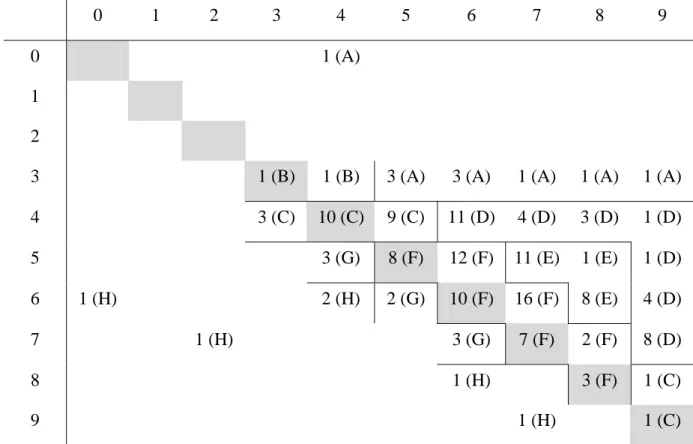
(2002), there were 187 subjects participating in sessions with a low-scale and a real high-scale treatment. 162 of these subjects behaved in a way that is consistent with expected utility theory. For two subjects the original data table reports eleven decisions in one of the treatments, which must be a typo. We exclude these subjects from our analysis.4 This leaves us with 160 subjects for whom we can analyze whether their behavior is consistent with CRRA. In Table 2, rows count the number of safe choices in the low-stake treatment while columns count the number of safe choices in the high-stake treatment. For the purpose of testing whether RRA is constant, increasing or decreasing, we can join the data from sessions with s=20, 50, and 90.5

Distribution of Choices (Data from Holt and Laury, 2002)

0 1 2 3 4 5 6 7 8 9

0 1 (A)

1

2

3 1 (B) 1 (B) 3 (A) 3 (A) 1 (A) 1 (A) 1 (A)

4 3 (C) 10 (C) 9 (C) 11 (D) 4 (D) 3 (D) 1 (D) 5 3 (G) 8 (F) 12 (F) 11 (E) 1 (E) 1 (D) 6 1 (H) 2 (H) 2 (G) 10 (F) 16 (F) 8 (E) 4 (D) 7 1 (H) 3 (G) 7 (F) 2 (F) 8 (D) 8 1 (H) 3 (F) 1 (C) 9 1 (H) 1 (C)

Table 2. Rows indicate the number of safe choices in the low-stake treatment, columns indicate the number of safe choices in the high-stake treatment. Letters in parentheses refer to the groups explained below.

103 subjects are counted in cells above the diagonal. They made more safe choices in the high-stake treatment than in the low-stake treatment. 40 subjects are counted on the diagonal:

4

Instructions and data tables are available from Susan Laury’s website at http://www2.gsu.edu/~ecoskl/. The two subjects excluded from our analysis are H2 and H6.

5

A detailed analysis of the wealth levels, at which observed choices are consistent with constant, increasing or decreasing RRA is available at http://www.sfm.vwl.uni-muenchen.de/heinemann/publics/measuring-ra.htm.

they made the same choices in both treatments. 17 subjects below the diagonal have chosen more of the risky options in the high-stake treatment than for low payoffs.

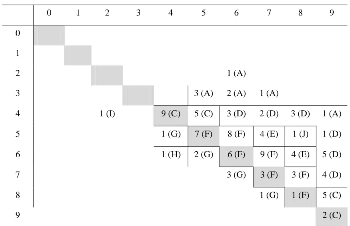
Harrison et al. (2005) had 123 subjects participating in their 1x10x treatment. 102 of these subjects behaved consistent with expected utility maximization, i.e. never switched from R to S for increasing p.

Distribution of Choices (Data from Harrison et al., 2005)

0 1 2 3 4 5 6 7 8 9 0

1

2 1 (A)

3 3 (A) 2 (A) 1 (A)

4 1 (I) 9 (C) 5 (C) 3 (D) 2 (D) 3 (D) 1 (A) 5 1 (G) 7 (F) 8 (F) 4 (E) 1 (J) 1 (D) 6 1 (H) 2 (G) 6 (F) 9 (F) 4 (E) 5 (D) 7 3 (G) 3 (F) 3 (F) 4 (D) 8 1 (G) 1 (F) 5 (C) 9 2 (C)

Table 3. Rows indicate the number of safe choices in the low-stake treatment, columns indicate the number of safe choices in the high-stake treatment. Letters in parentheses refer to the groups explained below.

65 subjects are counted in cells above the diagonal, 28 subjects are counted on the diagonal, and 9 subjects below the diagonal. In the remainder of this section we refer to the data by Holt and Laury (2002) without brackets and to data from Harrison et al (2005) in brackets []. To count how many subjects behave in accordance with CRRA, we sort subjects in 10 groups indicated by letters A to J in Tables 2 and 3. The number of subjects belonging to these groups is given for the data from Holt & Laury.

A. Group A contains 10 [8] subjects. Their behavior implies increasing RRA at all wealth levels.

B. Group B contains 2 [0] subjects. Their behavior is consistent with CRRA at W =0. For W >5 their behavior is consistent only with increasing RRA.

C. Group C contains 24 [21] subjects. Their behavior is consistent with constant, increasing or decreasing RRA at all wealth levels.

D. Group D contains 32 [18] subjects. Their behavior is consistent with increasing RRA at all wealth levels and with constant or decreasing RRA at all wealth levels W >50. It is inconsistent with non-increasing RRA at W =0.

E. Group E contains 20 [8] subjects. Their behavior is consistent with increasing RRA at 0

=

W , with decreasing RRA for W >50, and with CRRA for some wealth level in the range 0<W <50. It is inconsistent with non-increasing RRA at W =0 and with non-decreasing RRA at W >50.

F. Group F contains 58 [37] subjects. Their behavior is consistent with decreasing RRA at all wealth levels and with constant or increasing RRA at W =0. It is inconsistent with non-decreasing RRA at W >15.

G. Group G contains 8 [7] subjects. Their behavior is inconsistent with increasing RRA at all wealth levels. It is consistent with CRRA at W =0. For W >0 their behavior is consistent only with decreasing RRA.

H. Group H contains 6 [1] subjects. Their behavior implies decreasing RRA at all wealth levels.

I. Group I contains 0 [1] subject. Her or his behavior is consistent with constant, increasing and decreasing RRA if W >5. W <5 implies increasing RRA.

J. Group J contains 0 [1] subject. Her or his behavior is consistent with constant, increasing and decreasing RRA for 2<W <1000. W <2 implies decreasing RRA,

1000 >

W implies decreasing RRA.

Summing up, the behavior of 144 [93] out of 160 [102] subjects (90% [91%]) is consistent with CRRA at some wealth level (groups B – G, I – J).

For 62 [35] subjects (39% [34%]) a wealth level of W =0 implies an increasing RRA (groups A, D, E, I), for 6 [2] subjects (4% [2%]) W =0 implies decreasing RRA (groups H, J).

Realistic wealth levels are certainly all above $50. For 92 [53] subjects (57.5% [52%]) 50

>

W implies decreasing RRA (groups E – H), and only for 12 [8] subjects (7.5% [8%]) a realistic wealth level implies increasing RRA (groups A – B).

This analysis shows that the data do not provide firm grounds for the hypothesis that RRA is increasing in the scale of payoffs. There seems to be more evidence for the opposite conclusion: most subjects’ behavior is qualified to reject constant or increasing RRA in favor of decreasing RRA at any realistic wealth level.

Decreasing RRA is a possible explanation for behavior in low-stake and high-stake lottery decisions in the experiment. An alternative explanation is that subjects do not fully integrate their wealth with the prospective income from lotteries. Cox and Sadiraj (2004) suggest a two-parameter utility function

U(W,x)=sgn(1−r)(δW +x)1−r, (3) where W is initial wealth, x is the gain from a lottery, and δ is a parameter thought to be smaller than 1 that rules the degree to which a subject integrates initial wealth with prospective gains from the lottery. Parameter r is the curvature of this function with respect to δW +x. Although the functional form is similar to CRRA, r cannot be interpreted as the Arrow-Pratt measure of RRA, as will be explained below. Cox and Sadiraj (2004) provide an example to show that the puzzle raised by Rabin (2000) can be resolved if δW is close to 1. In the experiment, we do not know subjects’ wealth W. Hence, δ is not identified. But, we can estimate integrated wealth δW by the same method that we applied for analyzing wealth levels at which observed behavior is consistent with CRRA. Each cell in Tables 2 and 3 is associated with a range for integrated wealth δW that is consistent with utility function (3). From the previous analysis we know already that the behavior of 90% of all subjects, who never switch from R to S for increasing p, is consistent with (3) at some level of integrated wealth. Going through all cells and counting at which wealth levels their behavior is consistent with (3), yields the result that the proportion of subjects whose behavior is consistent with (3) has a maximum at δW ≤1.

For δW =0, there are 49 [33] subjects whose behavior is consistent with (3) only for one particular value of r. The median subject shown in Figure 1 is such a case. Her behavior is consistent with (3) at δW =0 if only if r is precisely 0.4115. It is unlikely that more than 30% of all subjects have a degree of risk aversion that comes from a set with measure zero. It is much more likely that these subjects have a positive level of integrated wealth which opens a range for r at which behavior is consistent with (3). The proportion of subjects whose

behavior is robustly consistent with (3) at δW =0 drops to 25% [27%], and we get a unique maximum for this proportion at δW =1.

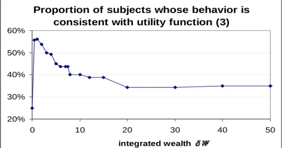
We illustrate this proportion in Figures 2 and 3 for the two data sets. Some subjects’ behavior is consistent with (3) only for sufficiently high levels of δW, while others require δW to be small. For 55% [51%] of all subjects behavior is consistent with (3) if and only if δW <50. Thus, it seems that most subjects integrate initial wealth in their evaluation of lotteries only to a very small degree.

Proportion of subjects whose behavior is consistent with utility function (3)

20% 30% 40% 50% 60% 0 10 20 30 40 50 integrated wealth

Figure 2. Proportion of subjects whose behavior is consistent with utility function (3). Non-robust cases counted as inconsistent. Data from Holt and Laury (2002).

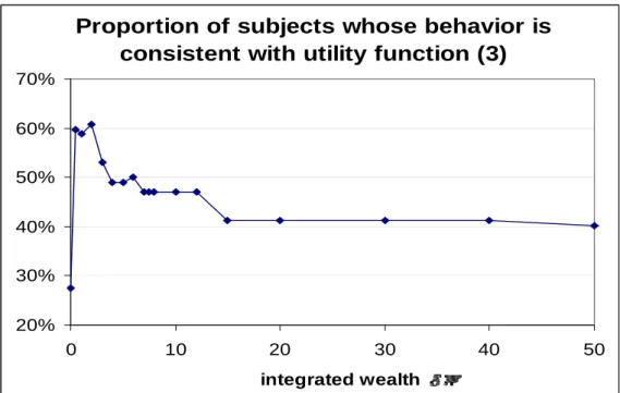
Proportion of subjects whose behavior is consistent with utility function (3)

20% 30% 40% 50% 60% 70% 0 10 20 30 40 50 integrated wealth

Figure 3. Proportion of subjects whose behavior is consistent with utility function (3). Non-robust cases counted as inconsistent. Data from Harrison et al. (2005).

Let us now analyze what this means for the question of whether RRA is increasing or decreasing. The answer may depend on how we define RRA for this utility function. The Arrow-Pratt measure is defined by RRA=−yU ''(y)/U'(y), where y is the single argument in the indirect utility function comprising initial wealth with potential gains from lotteries. Utility function (3) has two arguments, though. Suppose that δ is a positive constant. Then one might define RRA by the derivatives of (3) with respect to W or x.

RRAW = = ∂ ∂ ∂ ∂ − W U W U W / / 2 2 x W W r + δ δ (4)

is increasing in W if r>0 and decreasing if r<0. Thus, increasing wealth increases the curvature of the utility function with respect to wealth.

RRAx = = ∂ ∂ ∂ ∂ − x U x U x / / 2 2 x W x r + δ (5)

is increasing in x if r>0 and decreasing if r<0. Thereby, increasing the scale of lottery payments x increases the absolute value of this measure of RRA for all subjects who are not risk neutral. Following Binswanger (1981), we may call RRAx “partial RRA,” because it

defines the curvature of the utility function with respect to the potential income from the next decision only.

RRAW is the curvature of the utility function with respect to wealth, which is relevant for portfolio choice and all kinds of normative questions. While the absolute value of RRAW is

increasing in W, it is decreasing in x. This means that increasing the scale of lottery payments reduces RRAW. This reconciles the results for utility function (3) with the previous result that

for fully integrated wealth, risk aversion must be decreasing to explain the predominant behavior. On the other hand, the absolute value of partial risk aversion is decreasing in W. Thus, subjects with a higher wealth should (on average) accept more risky bets.

These properties are inherent in utility function (3) and can, therefore, not be rejected without rejecting utility function (3). As we laid out before, 90% of the subjects who never switch from R to S behave in a way that is consistent with (3). It follows that the experiment is not well-suited to discriminate between the two hypotheses: (i) agents fully integrate wealth and RRA is decreasing, and (ii) agents do not fully integrate wealth. Furthermore, if subjects do not fully integrate wealth, an experiment with lotteries of different scales cannot answer the question of whether RRA is increasing or decreasing in the wealth level.

Harrison et al. (2005) have shown that there is an order effect that leads subjects to choose safer actions in a high-scale treatment after participating in a low-scale treatment before than in an experiment that consists of the high-scale treatment only. This order effect may account for a substantial part of the observed increase in the number of safe choices in the high-scale treatments. Although the order effect does not reverse the responses to increasing scale, the numerical estimates are affected. If the increase in safe choices with rising payoff-scale had been smaller, then we would find less subjects in upper-right cells of Table 2 and more in cells, for which consistency with fully integrated wealth requires decreasing RRA. The proportion of subjects, whose behavior is consistent with utility function (3) would be shifted to the left, indicating an even lower level of integrated wealth. We infer that accounting for the order effect strengthens our results.

4 – Estimating a Hybrid Utility Function

Hybrid utility functions with more than two parameters cannot be estimated individually, if within-subject data are only elicited for lotteries of two different scales. In principle, one could do the same exercise with a third parameter, if subjects participate in lottery decisions

of three very distinct scales. However, between-subject data can be used to estimate models with more parameters than lottery scales. The obvious disadvantage of this procedure is that one assumes a representative utility function governing the choices of all subjects. Ideosyncratic differences are then attributed to “errors” and assumed to be random.

Holt and Laury (2002) apply such an error-response model. They assume a representative agent with a probabilistic choice rule, where the individual probability of choosing lottery S is given by μ μ μ / 1 / 1 / 1 )] ( [ )] ( [ )] ( [ R EU S EU S EU + . ) (⋅

EU is the expected utility from the respective lottery and μ is an error term. For μ→0 the agent chooses the option with higher expected utility almost certainly (rational choice). For μ→∞, the behavior approaches a 50:50 random choice. Utility is defined by a “power-expo” utility function

a x a x U r ) exp( 1 ) ( 1− − − = .

This function converges to CRRA for a→0 and to CARA for r→0. For x Holt and Laury insert the respective gains from lotteries. Again, they assume that initial wealth does not enter the utility function. We extend this approach by including a parameter for integrated wealth, i.e. we use a utility function

a x W a x W U r ) ) ( exp( 1 ) , ( 1− + − − = δ , (6)

where δW is integrated wealth and x is replaced by the respective gains from lotteries. As in the previous analysis, lack of data for personal income prevent an estimation of δ . Instead we may treat δW as a parameter of the utility function that is identified. Following Holt and Laury (2002), we estimate this model using a maximum likelihood procedure.

Table 4 reports the results of these estimates, in the first row for data from all subjects in the Holt-Laury sample, in the second considering only data from subjects, who never switch from R to S for increasing p, in the third row for the data from Harrison et al. (2005). Rows 4 to 6 contain the estimates of Holt’s and Laury’s model, which has the additional restriction of

W

two subjects that we omitted, because of typos in the data table. Numbers in parentheses denote standard errors.

Estimated parameters of the error response model

μ r a δW

Data from Holt and Laury (all subjects) .1161 (.0064) .324 (.0253) .0326 (.00325) .188 (.069) Date from Holt and Laury (subjects

who never switch from R to S for increasing p) .1060 (.0059) .313 (.0251) .0330 (.00315) .052 (.062)

Date from Harrison et al. (subjects who never switch from R to S for increasing p) .1095 (.0091) .0100 (.033) .0505 (.0045) .439 (.227)

Data from Holt and Laury (all subjects) .132 (.0046) .274 (.0174) .0286 (.00246) Date from Holt and Laury (subjects

who never switch from R to S for increasing p) .110 (.0041) .297 (.0167) .0316 (.00260)

Date from Harrison et al. (subjects who never switch from R to S for increasing p) .1266 (.0061) .0040 (.0233) .0492 (.0033) Table 4.

For samples restricted to subjects whose behavior is consistent with maximizing expected utility, we cannot reject the hypothesis δW =0. But, even for the total sample by Holt and Laury, the estimated asset integration is very close to zero (Recall that for full asset integration, δW should be above 100,000). Thereby, Holt’s and Laury’s assumption that a representative individual does not integrate wealth (δ =0) is obtained as a result.

Note that for δW =0, utility function (6) implies that partial RRA is increasing in x. On the other hand, partial RRA is decreasing in W if 0 < r < 1 and δ >0. We may conclude that partial RRA is increasing in the scale of lottery payments but not in wealth.

RRAW is zero for δ =0. This seems to imply a CRRA with respect to wealth. This conclusion is rash, though. Since subjects do not integrate wealth at all, the experiment is inappropriate to measure how risk aversion depends on wealth.

It is worth noting that the data from Harrison et al. (2005) do not support the hybrid utility function. The estimated value of r is not significantly different from 0. Thus, their data are consistent with constant partial absolute risk aversion.

5 – Conclusion

The extent to which subjects integrate wealth with potential income from lottery decisions in laboratory experiments is identified if subjects participate in lottery decisions with small and large payoffs and enter both decisions with the same wealth. To avoid order effects, these decisions should be made simultaneously, for example by using two multiple-price lists with different scaling factors and then randomly selecting one situation for payoffs. Although the experiment by Holt and Laury (2002) suffers from an order effect, their within-subject data indicate that most subjects either have a decreasing RRA or integrate their wealth only to a very small extent.

Within-subject data do not allow us to discriminate between these two hypotheses. However, the calibrations provided by Rabin (2000) do not rely on any assumptions about increasing or decreasing risk aversion. Behavior in low and medium-stake lotteries (as employed in experiments) can be reconciled with observed behavior on financial markets only, if initial wealth is not fully integrated in laboratory decisions.

One possible explanation for the disintegration of wealth with laboratory income can be found in mental accounting6: subjects treat an experiment and each decision situation as one entity for which they have an aspiration level that they try to achieve with low risk. This kind of "myopic risk aversion" has found strong support in an experiment by Gneezy and Potters (1997). The dark side of this explanation, however, is that mental accounting opens a Pandora-box to providing context-specific explanations for all kinds of behavior and severely limits the outside validity of experiments.

Subjects who do not integrate wealth treat each decision situation as being to some degree independent from other (previous) decisions, even though the budget constraint connects all economic decisions. They behave as if wealth from other sources is small in comparison to

6

Thaler (1999) and Rabin and Thaler (2001) provide nice surveys of these arguments. Schechter (2005, Footnote 2) provides anecdotal evidence for mental accounting.

the amounts under consideration in a particular decision situation. We have formalized this by assuming that a subject considers only a fraction δ of wealth from other sources in each decision. In our analysis, we have assumed that δ is a constant parameter. However, it seems perfectly reasonable that δ might be higher, if a subject has more reasons to consider her wealth in a particular decision. For example, Holt and Laury (2002) observe that the number of safe choices in high-stake treatments with hypothetical earnings was significantly lower than in high-stake treatments with real earnings. This may be explained by δ being higher in situations with real earnings.

Myopic risk aversion has interesting consequences for behavior in financial markets: with myopic risk aversion, people do not integrate their wealth with the potential income from financial assets that they decide to buy or sell. A person who does not integrate income from other sources in any particular decision has no reason to consider the correlation between the payoffs of different assets and evaluates each asset only by the moments of the distribution of this asset’s returns. Her decision is independent from the distribution of returns from other assets. There are some observations that point into this direction: for example the fact that many employees hold shares from the company that employs them. But, we also observe the desire to spread risks by holding a diversified portfolio. This indicates that in “very-large-scale” lotteries δ is positive.

It is an interesting question for future research under which circumstances subjects consider a substantial part of their wealth in decisions. Gneezy and Potters (1997) have gone so far as to draw practical conclusions for fund managers from the observed disintegration or “myopic behavior” as they call it. However, it is an open question whether and to what extend the framing of a decision situation raises the awareness that decisions affect final wealth. This awareness might be systematically higher for decisions in financial market than for lottery choices in laboratory experiments. A worthwhile study could compare lottery decisions with decisions for an equal payoff structure where lotteries are phrased as financial assets.

Another possible explanation for disintegration of wealth in laboratory decisions is the high evaluation that humans have for immediate rewards. Decisions in a laboratory have immediate consequences: subjects get money at the end of a session or at least they get to know how much money they will receive. The positive or negative feedback (depending on outcome and aspiration level) affects personal happiness, although the absolute amount of money is rather small (for s=90 they win at most $346.50). By introspection, I would suggest that this feeling is much smaller for an unexpected increase in the value of a portfolio

by the same amount. People know that immediate rewards evoke emotions and the high degree of risk aversion exhibited in the lab may be a consequence of this foresight.7 Subjects try to maximize a myopic utility arising from immediate feedback. To test this hypothesis, one might compare behavior in sessions, where the outcome of a lottery is announced immediately after the decision, with sessions in which the outcome is announced much later. In both treatments, payments would have to be delayed for avoiding that time preference for cash exerts an overlaying effect.

References

Arrow, Kenneth (1971), Essays in the Theory of Risk-Bearing. Chicago, IL, Markham Publishing Company.

Binswanger, Hans P, (1981), “Attitudes Toward Risk: Theoretical Implications of an Experiment in Rural India,” The Economic Journal 91, 867-890.

Cox, James C., and Vjollca Sadiraj (2004), “Implications of Small- and Large-Stakes Risk Aversion for Decision Theory,” mimeo, available at

http://www.cebr.dk/Events%20submenu/2004/Spring/Conference%202004.aspx. Gneezy, Uri, and Jan Potters (1997), “An Experiment on Risk Taking and Evaluation Periods,” Quarterly Journal of Economics 112, 631-645.

Harrison, Glenn W., Eric Johnson, Melayne M. McInnes, and E. Elisabet Rutström (2005), “Risk Aversion and Incentive Effects: Comment,” American Economic Review 95, 897-901. Holt, Charles A., and Susan K. Laury (2002), “Risk Aversion and Incentive Effects,”

American Economic Review 92, 1644-1655.

Kahneman, Daniel and Amos Tversky (1979), ”Prospect Theory: An Analysis of Decision und Risk,” Econometrica 47, 263-291.

Kreps, David M. and Evan L. Porteus (1978), “Temporal Resolution of Uncertainty and Dynamic Choice Theory,” Econometrica 46, 185-200

Markowitz, Harry (1952), “The Utility of Wealth,” Journal of Political Economy 60, 151-158. Rabin, Matthew (2000), “Risk Aversion and Expected-Utility Theory: A Calibration

Theorem,” Econometrica 68, 1281-1292.

7

Rabin, Matthew, and Richard H. Thaler (2001), “Anomalies: Risk Aversion,” Journal of Economic Perspectives 15, 219-232.

Samuelson, Paul (1963), “Risk and Uncertainty: A Fallacy of Large Numbers,” Scientia 98, 108-113.

Schechter, Laura (2005) “Risk Aversion and Expected.Utility Theory: A Calibration Exercise,” mimeo.

Thaler, Richard H. (1999), “Mental Accounting Matters,” Journal of Behavioral Decision Making 12, 183-206.