Convolutional Neural Network based Malignancy Detection of Pulmonary Nodule on Computer Tomography

(1)

Convolutional Neural Network based

Malignancy Detection of Pulmonary

Nodule on Computer Tomography

A Thesis Submitted to the

College of Graduate and Postdoctoral Studies

in Partial Fulfillment of the Requirements

For the degree of Master of Science

in the Department of Electrical and Computer Engineering

University of Saskatchewan

Saskatoon, Saskatchewan

By

Yi Wang

c

(2)

Permission to Use

In presenting this thesis in partial fulfilment of the requirements for a Postgraduate degree from the University of Saskatchewan, I agree that the Libraries of this University may make it freely available for inspection. I further agree that permission for copying of this thesis in any manner, in whole or in part, for scholarly purposes may be granted by the professor or professors who supervised my thesis work or, in their absence, by the Head of the Department or the Dean of the College in which my thesis work was done. It is understood that any copying or publication or use of this thesis or parts thereof for financial gain shall not be allowed without my written permission. It is also understood that due recognition shall be given to me and to the University of Saskatchewan in any scholarly use which may be made of any material in my thesis.

Requests for permission to copy or to make other use of material in this thesis in whole or part should be addressed to:

Head of the Department of Electrical and Computer Engineering, 57 Campus Drive

University of Saskatchewan

Saskatoon, Saskatchewan S7N 5A9 Canada

OR Dean

College of Graduate and Postdoctoral Studies, Room 116 Thorvaldson Building, 110 Science Place, Saskatoon, Saskatchewan S7N 5C9

(3)

Abstract

Without performing biopsy that could lead physical damages to nerves and vessels, Com-puterized Tomography (CT) is widely used to diagnose the lung cancer due to the high sensitivity of pulmonary nodule detection. However, distinguishing pulmonary nodule in-between malignant and benign is still not an easy task. As the CT scans are mostly in relatively low resolution, it is not easy for radiologists to read the details of the scan image. In the past few years, the continuing rapid growth of CT scan analysis system has generated a pressing need for advanced computational tools to extract useful features to assist the radi-ologist in reading progress. Computer-aided detection (CAD) systems have been developed to reduce observational oversights by identifying the suspicious features that a radiologist looks for during case review.

Most previous CAD systems rely on low-level non-texture imaging features such as inten-sity, shape, size or volume of the pulmonary nodules. However, the pulmonary nodules have a wide variety in shapes and sizes, and also the high visual similarities between benign and malignant patterns, so relying on non-texture imaging features is difficult for diagnosis of the nodule types. To overcome the problem of non-texture imaging features, more recent CAD systems adopted the supervised or unsupervised learning scheme to translate the content of the nodules into discriminative features. Such features enable high-level imaging features highly correlated with shape and texture.

Convolutional neural networks (ConvNets), supervised methods related to deep learning, have been improved rapidly in recent years. Due to their great success in computer vision tasks, they are also expected to be helpful in medical imaging. In this thesis, a CAD based on a deep convolutional neural network (ConvNet) is designed and evaluated for malignant pulmonary nodules on computerized tomography. The proposed ConvNet, which is the core component of the proposed CAD system, is trained on the LUNGx challenge database to classify benign and malignant pulmonary nodules on CT. The architecture of the proposed ConvNet consists of 3 convolutional layers with maximum pooling operations and rectified linear units (ReLU) activations, followed by 2 denser layers with full-connectivities, and the architecture is carefully tailored for pulmonary nodule classification by considering the

(4)

problems of over-fitting, receptive field, and imbalanced data.

The proposed CAD system achieved the sensitivity of 0.896 and specificity of 8.78 at the optimal cut-off point of the receiver operating characteristic curve (ROC) with the area under the curve (AUC) of 0.920. The testing results showed that the proposed ConvNet achieves 10% higher AUC compared to the state-of-the-art work related to the unsupervised method. By integrating the proposed highly accurate ConvNet, the proposed CAD system also outperformed the other state-of-the-art ConvNets explicitly designed for diagnosis of pulmonary nodules detection or classification.

(5)

Acknowledgements

I would first like to express my deep sense of thanks and gratitude to my supervisor Dr. Seokbum Ko of the Department of Electrical and Computer Engineering at the University of Saskatchewan. I was extremely lucky to have a supervisor who always willing to help me in all the time of research and writing of this thesis. Without his patience and knowledge, I would not have been accomplished the work presented in the thesis.

I also would like to thank my lab members, Hao Zhang, Zhexin Jiang, Juan Yepez and Suganthi Venkatachalam who helped me throughout my experiments. In particular, I am grateful to Hao Zhang for providing precious comments on this work.

Last but not the least, I would like to thank my parents for their continuous supports and encouragements throughout the period of writing this thesis.

(6)

List of Tables

2.1 Characteristics of the pulmonary nodules in LUNGx Challenge database . . 7

4.1 Receptive field of each learnable layer in proposed ConvNet . . . 37

4.2 Dataset distribution . . . 43

5.1 Performance of the ConvNets with Different Configurations . . . 46

5.2 Comparison of the proposed CAD system with the previous work . . . 50

5.3 Comparison with other ConvNet architectures . . . 50

5.4 Data distribution for original database and further augmented database . . . 55

(9)

List of Figures

1.1 A lung CT scan from a 64-year-old female. . . 2

1.2 A typical CAD system to detect malignant pulmonary nodule from CT scan. 4 2.1 Description of the spatial coordinate of a malignant nodule labeled by the six radiologists from LUNGx group. . . 8

2.2 A mathematical model of artificial neuron with three input nodes, x0, x1 and x2. . . 10

2.3 A 3-layer artificial neural network which consists of one input layer with two neurons, one hidden layer with three neurons and one output layer with a single neuron. . . 12

2.4 Classification performance on the different number of layers. . . 13

2.5 An example of convolutional layer to extract features within local region of the cropped image. . . 15

2.6 An example of max pooling operation. . . 17

3.1 Visual representations of the pulmonary nodule patches in axial view. . . 24

3.2 Schematic of the Shallow ConvNet. . . 25

3.3 Schematic of the ConvNet with two convolutional layers. . . 26

3.4 Schematic of the ConvNet with two grouped convolutional layers. . . 28

3.5 Schematic of the ConvNet with three convolutional layers. . . 29

3.6 Schematic of the AlexNet. . . 30

4.1 Overview of the proposed CAD system. . . 32

4.2 Extracted ROIs from LUNGx Challenge database. . . 34

4.3 Example of the receptive fields in a network with two convolutional layers. . 38

4.4 Architecture of proposed ConvNet. . . 39

4.5 Network with three fully-connected layers applies dropout with a ratio of 0.5. 40 4.6 Dataset distribution for the training-validation-test scheme of the proposed ConvNet compared to the LUNGx Challenge training-test scheme. . . 42

5.1 Training losses and validation accuracies during the training of the proposed system. . . 48

5.2 Example of ROIs that were classified or misclassified by the proposed ConvNet. 49 5.3 ROC curves for different ConvNet architectures. . . 59

(10)

List of Abbreviations

AUC Area Under the Curve

ANN Artificial Neural Network

CAD Computer-Aided Detection

CT Computerized Tomography

ConvNet Convolutional Neural Network

DNN Deep Neural Network

DICOM Digital Imaging and Communication in Medicine

HOG Histogram of Gradient

kNN K-nearest Neighbors

LBP Local Binary Pattern

LD Linear Discriminant

ILD Interstitial Lung Disease

PCA Principle Component Analysis

RBM Restricted Boltzmann Machine

ReLU Rectified Linear Unit

ROC Receiver Operating Characteristi

ROI Region of Interest

SIFT Scale-invariant Feature Transform

SVM Support Vector Machine

(11)

Chapter 1 Introduction

Lung cancer is becoming the most common cancer disease in the world. According to the statistical data published by the American Cancer Society [1], lung cancer is the leading cause of cancer death. Early detection and diagnosis is a meaningful way to increase the survival rate of cancer. In the field of lung cancer diagnosis, a patient who is suspected of having lung cancer is recommended to perform a chest X-ray at first because of low cost and simplicity to take. Lung cancer comes from the pulmonary nodule described as masses of abnormal tissue inside the lung. When the pulmonary nodule projects into X-ray image, the mass have different areas of density compared to the healthy tissues. By noticing the changing of the area of the density, the radiologist can find the location of lung cancer. However, a chest X-ray is a 2-dimensional projection of the lung, and the size of the pulmonary nodule is usually less than 10 mm. Therefore, it is difficult for the radiologist to confirm the types of the nodule (i.e., benign or malignant) and the exact nodule location to perform a further medical treatment. If the radiologist notices any suspicious finding in the chest X-ray, a further computerized tomography examination is suggested to finalize the diagnosis.

1.1 Pulmonary Nodule on Computer Tomography

Computerized Tomography (CT) scan, due to its high sensitivity to detect pulmonary nod-ules, is widely used by radiologists. It shows a higher detection rate compared to other chest radiography methods and is thus helpful in reducing the lung cancer mortality [59]. To over-come the problem of the chest X-ray, CT scanner analyzes the patient’s lung by performing many X-ray measurements with various angles and produces cross-sectional images of the lung. By combining the scanned CT images, the radiologist reviews the patient’s lung in

(12)

3-dimensional space. In contrast of X-ray image, CT images have a sophisticated metric (as referring to Hounsfield Units) to help radiologist distinguish patterns in-between abnormal and normal tissues.

In order to perform a completed CT scan, the CT scanner slowly slides along the axial axis from the patient’s head to the feet. As indicated in Figure 1.1(a), one CT scan gener-ates a series of cross-sectional images where start from the top to the bottom of the lung. Each acquired cross-sectional image from CT scanner is called a slice. Figure 1.1(b) and Figure 1.1(c) show two different slices acquired at different axial positions from a 64-year-old female patient, who has lung cancer, respectively.

C T S ca n D ir ec ti on Top of Lung Bottom of Lung (b) Normal Slice (c) Abnormal Slice (a) A CT Scan

Figure 1.1: A lung CT scan from a 64-year-old female [26]. (a) direction of acquiring slices. (b) one normal slice. (c) one abnormal slice which contains a malignant nodule on the right top of the right lobe.

1.2 Computerized diagnosis of pulmonary nodule

In practice, although the CT scans have high sensitivity in the pulmonary nodule detection [60], it is still not easy for a radiologist to determine whether the nodule belongs to benign or

(13)

malignant. When the amount of patient cases is significant, it takes time for the radiologist to make the diagnosis. The seminal National Lung Screening Trial [60] reported mortality from lung cancer was reduced 20% by screening low-dose CT scans. However, the rate of positive low-dose CT scans was 24.2%, while a total of 96.4% of positive screenings showed a false positive. According to [60], a false positive diagnosis will lead to unnecessary follow up medical examinations which will delay the diagnosis while increased radiation exposure causes further damage to the patient.

Computer-Aided Detection (CAD) systems have been developed to reduce observational oversights by identifying suspicious features that a radiologist looks for during case review. Because the CAD system improves the accuracy of diagnosis by radiologists, the CAD system becomes a good choice for preliminary diagnosis [27, 44, 45, 11, 18, 4, 50, 31, 22, 69, 46, 2, 41, 25].

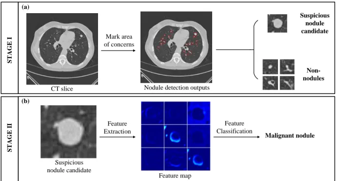
A typical CAD system for a lung CT scan consists of two stages: 1) nodule detection and 2) lung disease classification. The first stage refers to marked areas of concern which highlight suspicious nodule candidates. To generate marks, general approaches are applied through image processing methodologies such as double threshold metrics or morphology operations [27],[44]. However, marks generated by CAD systems generally have high sensitivities and false positive rates [11]. Therefore, the second stage aims to reduce false positive rates for marked areas of concern, while providing the capability of clinical diagnostic decision making. Typically, features from marked areas of concern are extracted, and machine learning schemes are used for nodule classification [27, 44, 45]. Figure 1.2 illustrates a completed CAD system to help clinical radiologist for diagnosis of pulmonary nodules.

1.3 Motivation

A computer-aided diagnosis tool related to malignancy grading of pulmonary nodule belongs to the second stage of the CAD system and focuses on reducing the false positive rate by distinguishing the nodule types in-between benign and malignant cases. Pulmonary nodules have a wide variety of shapes and sizes, as well as high visual similarities between benign and malignant patterns, so analyzing low-level non-textual characteristics such as shapes or

(14)

Mark area of concerns Suspicious nodule candidate Non-nodules

CT slice Nodule detection outputs

Feature Extraction Suspicious nodule candidate Feature map Feature Classification Malignant nodule S T A GE I S T AGE I I (a) (b)

Figure 1.2: A typical CAD system to detect malignant pulmonary nodule from CT scan. (a) overview of stage 1 on nodule detection. (a) overview of stage 2 on lung disease classification.

sizes of the nodules always fail to provide a promising diagnostic performance. Early devel-oped CAD system for pulmonary nodule detection applied conventional imaging processing methods to describe the low-level features of the pulmonary nodule in the higher dimensional spaces [18, 4, 50, 31]. However, such features had limited generalizations when new nodule patterns appeared due to low discriminative power [47].

In recent years, deep learning has achieved great success in image classification, objective detection, image segmentation, and natural language processing. In many of these fields, deep learning can achieve near human performance [53]. Convolutional neural network (ConvNet), the most popular deep learning architecture to perform image classification, has the ability to extract high-level discriminative features. In addition to clinical usage for pulmonary nodule detection, ConvNet uses the patch-based raw image without any additional information such as nodule segmentation or volume of the nodule, and the ConvNet is trained automatically end-to-end in a supervised manner without any additional feature extractor or classifier. Thus, ConvNet is expected to be helpful in improving the performance of CAD systems. Many research works have been done to utilize deep learning in medical field [36, 39, 13, 55,

(15)

37, 68] to achieve higher accuracy of diagnosis.

1.4 Aim of Thesis

This thesis aims to design a CAD system based on a ConvNet for diagnosis of the malignant pulmonary nodule on CT scan. The designed ConvNet is able to distinguish pulmonary nodules in-between benign or malignant through raw input image without the need of ad-ditional segmentation. To achieve the aim of this thesis, the designed ConvNet is carefully tailored for pulmonary nodule classification task by: 1) exploring optimal hyper-parameters including filter size, receptive field, and optimizer. 2) investigating the performance im-pact of the imbalanced training dataset. 3) comparing the classification performance with the state-of-the-art work without interference of ConvNet [46] and other related solutions [36, 37, 55, 68, 58].

1.5 Thesis Outline

The rest of the thesis is organized as follows: Chapter 2 introduces the LUNGx Challenge public database used to train and evaluate the proposed CAD system, followed by the theories of the ConvNet including layer operations and training optimization. Chapter 3 presents the current state-of-the-art works for malignancy detection of the pulmonary nodule on CT scan. Chapter 4 introduces the methodologies of the proposed CAD system for pulmonary nodule detection. Chapter 5 presents requirements to set up the experiments and the evaluation comparisons of unsupervised learning method and other ConvNet architectures from previous studies, followed by an analysis of imbalanced data problem that is commonly occurred in the medical imaging database. Finally, Chapter 6 concludes the thesis.

(16)

Chapter 2 Background

The purpose of this chapter is to introduce the lung CT database used to train and evaluate the proposed ConvNet, followed by relevant theories about the proposed convolu-tional neural network. The definition of the input database and ConvNet provide a better understanding regarding the implementation of the proposed CAD system.

2.1 LUNGx Challenge Database

LUNGx Challenge database [26] was used for LUNGx Challenge [3], which was a challenge to seek novel CAD systems for classification of pulmonary nodules on diagnostic computerized tomography scans as benign and malignant. During the LUNGx Challenge event, six expe-rienced radiologists attended the event by manually performing nodule malignancy ratings. As reported in [3], the diagnostic area under the curve (AUC) from the six radiologists is ranged from 0.70 to 0.85 with a mean AUC of 0.79, and three of the six radiologists have statically better performance on malignancy detection compared to the submitted CAD sys-tems during the LUNGx challenge event. Although LUNGx challenge was ended in 2016, malignancy detection of the pulmonary nodule on LUNGx database is still challenging.

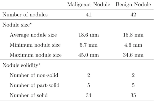
The characteristics of the pulmonary nodules in LUNGx Challenge database is shown in Table. 2.1. The LUNGx Challenge database collect 41 malignant nodules, and the size of the malignant nodule is in the range between 5.7 mm and 45.0 mm with the average size of 18.6 mm. In addition to nodule solidity, 34 malignant nodules are categorized into the group of the solid nodules which its Hounsfield Units (HU) on CT are above -450. 2 malignant nodules demonstrate the characteristic of the non-solid nodule with lower HU intensity which has a range from -750 to -300. There have 5 malignant nodules which belong to part-solid nodules,

(17)

and the part-solid nodule consists of a solid and a non-solid part. On the other hand, in the LUNGx Challenge database, 42 nodules belongs to benign cases. The smallest benign nodule is 4.6 mm, and the largest one has the size of 34.6 mm. Among the entire benign cases, there are 35 solid, 2 non-solid and 5 part-solid nodules.

Table 2.1: Characteristics of the pulmonary nodules in LUNGx Challenge database

Malignant Nodule Benign Nodule

Number of nodules 41 42

Nodule size?

Average nodule size 18.6 mm 15.8 mm

Minimum nodule size 5.7 mm 4.6 mm

Maximum nodule size 45.0 mm 34.6 mm

Nodule solidity?

Number of non-solid 2 2

Number of part-solid 5 5

Number of solid 34 35

? _{All the data of nodule sizes and nodule solidities is provided by}

LUNGx organizers [3], and the nodule size is measured by follow-ing the Response Evaluation Criteria in Solid Tumors (RECIST) guidelines [61].

Each CT scan from the LUNGx Challenge database is obtained under 120kV or 140kV tube peak potential energy with tube current in the range from 240 to 500 mA and tube current-exposure time product of 200-325 mA. The CT scans are reconstructed to the digital

imaging and communication in medicine (DICOM) format having the spatial size of 512 ×

512 pixels. The DICOM files of each CT scan are reconstructed with no gap and consists of approximated 250 slices with the slice thickness of 1 mm.

The proposed CAD system is trained and evaluated by using LUNGx Challenge database. The database provides 60 test sets of full thoracic coverage CT scans with 10 calibration sets. The purpose of the calibration sets is to train the CAD systems designated for detecting

(18)

Axial axis (Slice Number) _{512 pixels}

512

p

ixe

ls

Central mass of the nodule at (X,Y,Z)

Central mass of the nodule at Z slice

(X,Y)

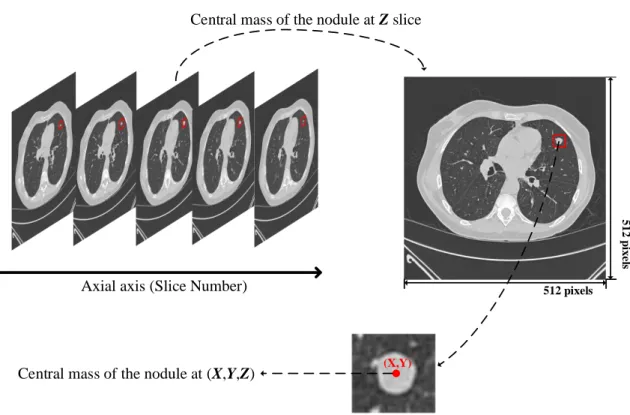
Figure 2.1: Description of the spatial coordinate of a malignant nodule labeled by the six radiologists from LUNGx group. The central coordinate of the malignant nodule in

the volume of CT scan is labeled as (x,y,z).

malignancy of pulmonary nodule, and the performances of the trained CAD systems are evaluated by using the 60 testing dataset as the inputs. Six experienced radiologists confirmed the 83 pulmonary nodules which consist of 42 benign nodules and 41 malignant nodules from the entire LUNGx Challenge database. The reference standard for each confirmed nodule was set via spatial coordinates of the approximate center of each nodule and diagnosis decision between benign and malignant. Figure 2.1 demonstrates the process of how the radiologists label each patient case on CT scan. The malignant nodule as shown in Figure 2.1 is labeled by finding the slice where appeared nodule is located at the center mass of the nodule volume. Because each slice is a cross-sectional image of the CT scan in the axial view, the nodule appears in a series of slice images, so the center mass of the nodule volume has an axial coordinate as referring to the slice number. After locating the slice number, the nodule exhibits as a 2-D image in the slice. By locating the center of the nodule in the slice, the

(19)

mass of the malignant nodule is located at the zth slice image where the nodule appears at

(x,y) in the spatial domain of the zth _{slice. By taking advantage of the labeled data which}

has already provided by LUNGx organizers, the nodule samples can be extracted. The detail of extracting the nodule samples is described in section 4.1.1.

2.2 Neural Networks

The artificial neural system brings the strong interest of emulating human brain with a size and complexity comparable model. Artificial neural network (ANN) has originally been interested in modeling neocortex on the biological nervous system but has recently applied to machine learning tasks such as voice recognition, computer vision, robotic control, and data mining. Deep neural network (DNN) is an improved ANNs model and capable of predicting data as accurate as human performance. DNN model consists of more layers than typical ANN; thus, DNN is able to extract high-level abstraction in data [35]. ConvNet is one type of DNN by employing convolution operations to extract image features. Since ConvNet is introduced in early 1990’s [34], it has demonstrated impressive image recognition on ImageNet [15] benchmark. In 2015, ResNet [24] has classified 1.2 million high-resolution images from ImageNet database that contains 1000 different classes with error rates of 3.57%.

2.2.1 Artificial Neuron

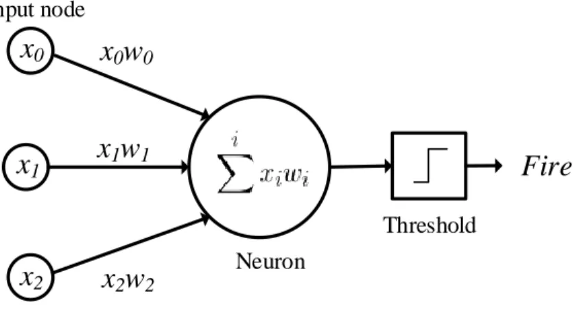
When we see an object via the eye, the light receptors in our eye send biological current through the optic nerve. Neurons in our brains process the biological current and let us know what the eye sees. Figure 2.2 illustrates a simplest artificial neuron which consists of three input nodes and produces a binary output.

Because the computer has different representations of the visual system than human, computer perceives image by constructing the image patterns with pixels. In Figure 2.2,

three image pixels (x0, x1 and x2) through unique synapses paths to generate synapses

current. Each synapse path contains a learnable weight (w0, w1 and w2) which interacts

multiplicatively with the input pixel. When our eye focuses on one object, our eye automati-cally ignores other objects where are surround us. Likely, learnable weights control synapses

(20)

x0

x1

x2

x0w0

x1w1

x2w2

Fire

Input node Threshold Neuron

Figure 2.2: A mathematical model of artificial neuron with three input nodes, x0,x1

and x2.

current to related image patterns. For example, by setting negative weights, inhibitory (neg-ative) synapses currents are generated to ignore unrelated image patterns. When input nodes consist of relating image patterns, excitatory (positive) synapses currents are generated. In the final stage of the model, the neuron receives and sums all synapses currents. If summed value exceeds a certain threshold, the neuron is fired. The output of the artificial neuron can be mathematically expressed as:

y=f(

i

X

xiwi+b) (2.1)

xi is the ith input,wi is the weight corresponding to ith input,bis bias andf is activation

function. Bias is a constant parameter summed before activation function. The idea of bias is that bias allows the cluster of the classifier to fit the data accurately [19]. For example, an output of the neuron cannot be fired regardless of changing learnable weights if the inputs are all zeros. However, most medical images are stored as gray-scale. In the representation of a gray-scale image, a pixel which has zero intensity corresponds to the black color. Therefore, by adding bias, the neuron can be fired even all input pixels are zeros.

Activation function uses to control the firing rate of the neuron by changing the threshold. Because activation function is a non-linear function, it statically compresses the output of the neuron in a finite range regardless of how large or small the output of the neuron is. Most common activation function are: sigmoid function (Eq. 2.2), tanh function (Eq. 2.3) or

(21)

rectified linear unit (Eq. 2.4).

f(x) = 1

1 +e−x (2.2)

f(x) =tanh(x) (2.3)

f(x) =max(x,0) (2.4)

2.2.2 Artificial Neural Networks

A collection of artificial neurons forms the layers of the ANN. The neurons from the previous layer build full-connections to each neuron in the next layer via synapse paths. A typical ANN consists of an input layer in which the size of neurons matches the number of input features, and it has one output layer used to generate scores of different classes. One or two hidden layers are employed in-between the input layer and the output layer to perform feature extraction [65]. The architecture of the DNN is inspired by integrating with deeper and denser hidden layers. Because DNN builds more complex synapse paths compared to ANN, increased capacity of learnable weights enables better learning abilities so that DNN is able to extract more features in higher level abstraction.

Figure 2.3 shows a simple ANN which takes two input features (x0 and x1) and consists

of three neurons (h0,h1 andh2) in the hidden layer. Such a 3-layer ANN structure is capable

of generating a single class score (y). For example, the risk of getting lung canner could

depend on family history of lung cancer and smoking history [43]. To evaluate the risk via ANN, the 3-layer ANN extracts the patient histories as two input features and outputs the score for the risk of getting lung cancer.

The ability to extract input features is that neurons are organized into layers, and the hidden layer uses to extract input features. In Figure 2.3, the hidden layer extracts three features regarding both input features. The extracted features are uncorrelated due to none of the synapse path with each other, but synapse paths build full-connections from two input features to each neuron in the hidden layer, so the extract features are correlated to both

(22)

Input layer Hidden layer Output layer x0 x1 y h0 h1 h2

Figure 2.3: A 3-layer artificial neural network which consists of one input layer with two neurons, one hidden layer with three neurons and one output layer with a single neuron.

input features. Then, neurons from the hidden layer pass the extracted features via synapse paths to the output neuron.

The process of propagating input features from the hidden layer (layers) to output layer is defined as feed-forward propagation [19]. The feed-forward propagation for 3-layer ANN can be defined as:

   hi =f(Pjxjwij1 +bi) y=f(Pi hiwi2+by) (2.5)

wherehi is the ith neuron in the hidden layer, xj is the jth input neuron,w1ij is the weight

in the synapse path where is from jth _{input neuron to i}th _{neuron in the hidden layer, and} _y

is the output neuron. The synapse path, from ith neuron in the hidden layer to the output

neuron, has weight of w2

i. bi and by are the biases for ith neuron in the hidden layer and the

output neuron respectively. f refers to activation function.

Deep Neural Networks

By propagating more stages (hidden layers) before reaching the output layer, such an ANN structure can be expressed as a DNN. Empirically, DNN, employs deeper hidden layers

(23)

com-pared to ANN, has more representational power for feature extraction and better general-ization for feature learning [19]. Figure 2.4 shows increasing the depth and width of each hidden layer yields increased test accuracy, which the experiment data is collected from [19].

Figure 2.4: Classification performance on the different number of layers [19].

Because deeper hidden layers statically increase the number of synapse paths, the deeper hidden layers extract more features via increased learnable parameters. For example, the 3-layer ANN, showed in Figure 2.3, adopts 4 neurons to extract input features, and it builds 9 synapse paths which consist of 9 learnable weight parameters with additional 4 bias param-eters for a total of 13 learnable paramparam-eters. By inserting additional two hidden layers with double size of neurons, the new architecture contains 16 neurons which build up 36 more synapse paths and 12 more bias parameters compared to the original 3-layer ANN. The total number of learnable parameters is increased by approximately 7 times. Therefore, DNN out-performs ANN for the statistical reason because adding and expanding hidden layers increase the number of learnable parameters dramatically.

Problems of Deeper Neural Network

When a shallow DNN with few hidden layers is trained, inserting more hidden layers does indeed to have better classification accuracy on the test dataset. However, the classification

(24)

performance eventually is saturated when the number of hidden layers exceeds a certain threshold (as referring to Figure 2.4).

As DNN consists of deeper hidden layers, such a model builds a more complicated func-tion (connecfunc-tion) in-between input features and outputs. On the other hand, over-fitting [33] occurs when the deeper layers easily accumulate an extensive collection of learnable param-eters. The learnable parameters with high capacity force the model to fit the training data perfectly by tunning the parameters to fit the noises in the training data. As a consequence, the model losses generalization on additional data.

Moreover, DNN builds full connectivities between two adjacent layers. Such a connection scheme forces the network to extract features based on entire input features. Therefore, trained model is lack of generalizing spatial invariance. For instance, trained images which apply rotation transformation result in inferior classification performance because the input features are shuffled via rotation.

2.2.3 Convolutional Neural Network

ConvNet is a particular type of DNN that employs convolution operation to extract features within the local spatial region of the image. Instead of building fully-connectivities in-between hidden layers, ConvNet forces hidden neurons to “see” local information and combine them to form high-level feature. Different features usually appear at various local regions because neighboring pixels are more correlated than faraway pixels. Therefore, ConvNet adopts a collection of local feature detectors to achieve tremendous success in image classification.

ConvNet stacks a sequence of layers to transform input images from pixel values to class scores. General ConvNet has four types of different layers: convolutional layer, activation layer, pooling layer and fully-connected layer.

Convolutional Layer

The convolutional layer adopts learnable filter banks. Each filter convolves full depth of the input volume within fixed-scale of spatial area, depending on filter size along with its width and height. Instead of building full connectivity from whole neurons on input volume to output neuron such as ANNs, the connection of the convolutional layer inspires feature

(25)

extraction within local regions of the input volume. On the other hand, a set of filter banks produce overlapping features extracted from a particular local region due to output depth of each filter. Such overlapping features offer various representations of the particular local region. Therefore, the output of the convolutional layer generates a group of feature maps, and each feature map corresponds to different local regions from input volume.

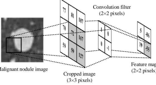
Malignant nodule image

Convolution filter (2×2 pixels) Feature map (2×2 pixels) Cropped image (3×3 pixels)

Figure 2.5: An example of convolutional layer to extract features within local region

of the cropped image. The convolutional layer consists of one filter of size 2×2 and

one output feature map.

Figure 2.5 shows a convolution operation for the cropped image by sliding the convolution

filter along the spatial matrix of size 3×3. For a convolutional layer, hidden neurons are

organized into each feature map. Unlike the DNN connection scheme (as referring to Fig-ure 2.3), each hidden neuron in the convolutional layer builds the connection to a particular local region of the input features. For example, the feature map, in Figure 2.5, consists of

4 hidden neurons to form a 2 ×2 matrix of the feature map, and each matrix element in

the feature map represents the output of each hidden neuron. By convolving the 2×2 filter

without flipping, the highlight area of the input features is extracted to a unique feature which is equal to -55 in the feature map. Hence, a local region of input features with the size

of 2×2 corresponds to one feature in the feature map. In general, the output of each hidden

(26)

yi,j = (x~w)(i,j)+bi,j or equivalently yi,j = X m X n x(i+m, j +n)w(m, n) +bi,j (2.6)

In order to extract the featureyi,j atith row and jth column of the feature map, weights

of the filter w with size of m×n perform dot production on the input features x from ith

row and jth _{column to (}_i₊_m₎th _{row and (}_j₊_n₎th _{column while the result of the dot product}

adds the bias term, bi,j.

Although the feature extraction scheme of the convolutional layer is inspired by the feed-forward propagation in ANN (as referring to Equation 2.5), the learnable parameters are dramatically reduced because a single feature map is generated by convolving the same filter, so each hidden neuron shares the learnable parameters from the same filter. Hence, ConvNet has fewer chances of having over-fitting due to sharing the learnable parameters. Moreover, ConvNet takes advantage of sharing parameters. Instead of relying on a denser hidden layer to extract as many features as possible, the convolutional layer avoids the trained model fit the input noises while learning the invariant relationships within the local spatial region by stacks a series of filters (filter banks).

Activation Layer

The convolutional layer is often followed by an activation layer. Instead of extracting learned features, the activation layer is used to introduce nonlinearity to the ConvNets in order to accelerate convergence during the training phase. Although a large amount of data and high-performance parallel computing solutions spurs ConvNets to integrate more convolutional layers in order to achieve better classification result, long training time is still an important concern. Most modern ConvNets architectures employed activation layer to reduce training time while maintaining similar performance. Typical activation layer produces non-linearity via sigmoid function, tanh function or ReLU.

Pooling Layer

It is common to insert a pooling layer between successive convolutional layers to reduce the spatial dimensionality of each feature map. Full connectivity structure used in ANN requires

(27)

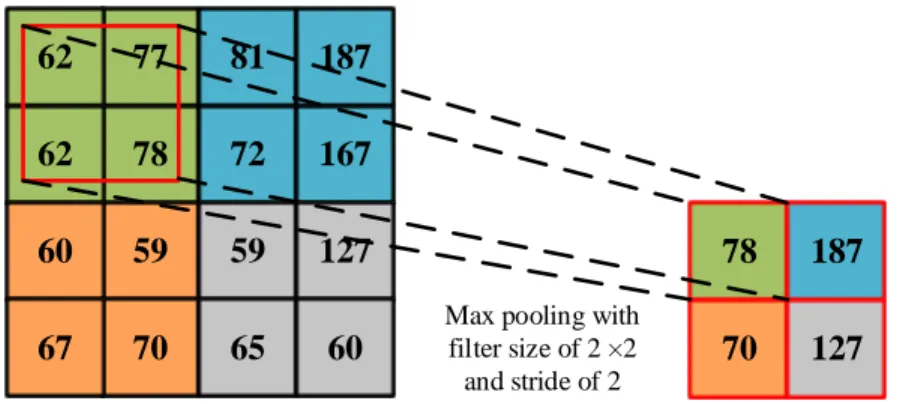
a large number of weight parameters to match high definition input scale which often leads to over-fitting. Also, the convolutional layer still has the chance to produce specific redundant information because the local region still builds full connectivity. Therefore, pooling layer retains the essential information and reduces chances of over-fitting. General pooling opera-tions are max-pooling or average-pooling by replacing input values to maximum or average value. 77 81 187 78 72 167 59 59 127 62 62 60 70 65 60 67

Max pooling with filter size of 2 ×2 and stride of 2

78 187 70 127

Figure 2.6: An example of max pooling operation. The 2×2 filter with a stride of 2 takes 4 inputs and perform down-sampling by retaining the maximum value.

Figure 2.6 illustrates a max pooling layer down-samples the input feature map. The

feature map of size 4×4 is pooled by retaining the maximum value within the pooling filter

which has the size of 2×2 and stride of 2. By keeping the maximum value of neighboring

features, the feed forward path of the ConvNet has less redundancy, and the path having max activation is also retained.

Fully-connected Layer

Fully-connected layer builds full connections to previous pooling layer. The fully-connected layer has a similar structure as ANN which performs classification. After last fully-connected layer, it is common to normalize the output vectors via SoftMax [7] function. The SoftMax can be defined as:

b yi = eyi Pj eyj (2.7)

(28)

where the SoftMax function suppresses the output vector at ith neuron to a value in-between zero and one via an exponential function. Then, by dividing the suppressed output

vector atithneuron with the sum of all suppressed output vectors in the layer, the normalized

output vector at ith _{neuron is generated and referred as}

b

yi. The normalized output vector

represents the probability distribution among all possible categories [7].

2.2.4 Training Convolutional Neural Network

Training the ConvNet corresponds to optimize the learnable parameters in convolutional layers and fully-connected layers so that the trained model fits the training data. Because the output of ConvNet produces the probabilistic distribution of the classes via SoftMax function, the input features that belong to a particular class most likely has the highest probability by feed-forward propagating the well-trained model. A standard optimization method of the ConvNet is to minimize the losses of the loss function.

Loss Function

In order to evaluate the classification performance in the training phase, a loss function is used to measure the errors between prediction scores and ground truths. For example, a malignant nodule image patch is fed into a ConvNet model, but the output of the ConvNet result in a higher score toward the class of benign nodule. To measure the error of the misclas-sification, the loss function intuitively produces a large loss regarding the misclassification. By utilizing the learnable parameters, the loss is gradually reduced while the ConvNet gets more confidence to classify the image patch as malignant. Because the malignancy detection of pulmonary nodule relates to binary classification, the loss function for the malignancy detection can be defined as the binary cross-entropy loss function:

Li =−fxi·log(fbxi)−(1−fxi)·log(1−fbxi) (2.8)

where the cross-entropy loss for ith _{input volume which consists of feature} _x

i is Li. fxi

refers to the ground truth label, andfb_x_i means the class score corresponding to the ith input

(29)

Optimizers

A loss function quantifies the quality of how well the model fits the training data. In order to achieve low losses, it is crucial to apply an appropriate optimizer to fine-tune learnable parameters so that the loss function is minima. A naive way of fitting the training data is to generate a large collection of random values, and the best model is obtained by trial-and-error. Instead of exhaustive searching the best learnable parameters, the gradient of the loss function provides a direction toward to minimal loss. The gradient of the loss function can be expressed as:

θ=θ−µ· ∇θL(θ) (2.9)

where the loss function is minimized with regards of a parameter,θ for an entire training

dataset. By moving θ in a descent direction of the gradient with constant steps, the losses

for the entire training dataset is gradually minimized. ∇θL(θ) refers to the gradient of the

loss function, and µ is the step size as referring to the learning rate.

Because the cross-entropy function is the part of Kullback-Leibler divergence [52] which is a convex function, applying a relatively large learning rate leads to high chances of missing the optimal point of the model. Conversely, a relatively small learning rate leads to a continuous reduction in the loss, but the model takes time to reach the optimal point with regards to convergence.

On the other hand, such a gradient descent algorithm (as referring to Equation 2.9) updates the learnable parameters by calculating the gradients of an entire dataset. When the size of the training data is large, a single update still requires a long time [49].

Stochastic Gradient Descent

Stochastic gradient descent (SGD) updates the gradient of the loss function based on each training sample or batch [8]. In contrast of the conventional gradient descent which performs redundant computations among the entire training dataset, SGD is much faster by performing frequent computations within a limited batch size. Instead of finding the global minimum point of the loss for the entire training dataset, SGD optimizes the model by converging to the local minimum points for each training sample or batch. Because the activation layer

(30)

introduces non-linearity, the cross-entropy loss has a shape of a non-convex surface, and the non-convex surface usually consists of several basins as referring to local minimal points. Thus, frequent updates of the local gradients in SGD leads the model to jump to a new local minima with a better loss, and the model eventually converges to the global minma. SGD

with regard to a parameter update θ can be defined as:

θ=θ−µ· 1

n · ∇θ

X

n

L(θ, xn, yn) (2.10)

where the loss function L computes the average of the cross-entropy losses from n training

samples {x1, ..., xn} with ground truth labels{y1, ..., yn}.

SGD refers to a batch based gradients, and the gradient of a batch loss mathematically represents as a non-convex surface so that the SGD contentiously keep overshooting (SGD fluctuation [49]). It is common to apply a step-down learning rate to control the direction of the gradient. A step-down learning rate applies a relatively large learning rate in the early stage of the training phase, so the speed of the convergence is accelerated. After several training iterations, the learning rate is decreased by order of magnitude. A reduction of the learning rate leads to consistent finding the best local minima which has the lowest loss. In order to have a smooth reduction of the learning rate, an exponential decay algorithm gradually decrease the learning after each epoch, and each epoch refers to the total number of iterations for the model to train the entire training dataset. The exponential decay of the learning rate can be expressed as:

µ=µ·e−γt (2.11)

whereγ is a hyper-parameter that refers to the decay rate. t is the iteration number.

Adaptive Optimizers

The hyper-parameters of the learning rate in SGD has to predefine before the training phase. Hence optimizing the learning rate in SGD is an expensive time cost progress. Adaptive opti-mizers (e.g., Adam [32], AdaGrad [16] or RMSProp [62]) adaptively adjust the learning rate based on the magnitude of the gradients [49]. Adaptive optimizers dynamically change the learning rate to perform more efficient gradient updates compared to non-adaptive optimizer

(31)

such as SGD. However, the adaptive optimizers lead the learning rate to shrink in one of the local minimal points so that the model will never reach the best optimal loss.

Back-propagation

Optimizers such as SGD point out the appropriate direction to achieve minimal loss of the loss function. In order to alter the weights and biases in each layer, a back-propagation provides an efficient way to find the gradients of each layer and recursively computes the gradients from the loss function to the first layer of the ConvNet. The gradient for each layer is estimated via chain rule of the derivation. Algorithm 1 presents the algorithm of back-propagation. The back-propagation is employed after computing the gradient of the loss function through optimizer such as SGD.

Algorithm 1 Back-propagation

whilecurrent iteration<maximum iterationsANDgradient of the loss function<desired

criterion do

for Input sample from training dataset do

Compute the gradient of the loss function through optimizer

for each hidden neurons in the output layer do

Compute gradient as error signal

end for

for each layer flow backward from output layerdo

Compute gradient of the layer Update bias parameter

for each hidden neurons in the layer do

Compute gradient of the hidden neuron Update weight parameter

end for end for end for end while

(32)

Chapter 3 Related works

Pulmonary nodule patterns are generally presented as unique texture inside lung lobe. Before deploying classification schemes, most CAD systems apply feature extraction opera-tions within the marked area of concern. Depending on the input scale of the classifier, the marked area of concern typically is generated as two different modalities: local regions of interest (ROIs) or volumes of interest (VOIs). By sliding fixed-scale of classifier over ROIs or VOIs, the diagnostic decision for pulmonary nodules is made.

3.1 Traditional Feature Extraction Approaches

Early studies demonstrated the usefulness of discriminative features to detect pulmonary nodule over ROIs or VOIs, such as first order gray-level thresholding operations [18, 4], histogram of gray-level [50] and histogram of CT density [31]. Since more modern texture descriptions were implemented, recently proposed CAD systems provided a new perspective of feature extractions in higher dimensional spaces. Such systems employed local binary pattern (LBP) [22], histogram of gradient (HOG) and scale-invariant feature transform (SIFT) [69].

3.2 Unsupervised Learning

The previously presented approaches for feature extractions relied on hand-crafted features which had lack of adaptabilities when new nodule patterns appeared. To achieve promising results against new data, more recent studies agreed with unsupervised feature learning. Such features allowed the systems to discover customized features regardless of input features. Such systems are k-means [13], principal component analysis (PCA) followed by convolution

(33)

and pooling operations [46], and restricted Boltzmann machine (RBM) [25] which is an unsupervised learning scheme adopted architecture of the artificial neural network (ANN).

Regardless of extracted features, it is also crucial to choose an appropriate classifier that optimally translates the features into correct classes. General feature-based classifiers applied for pulmonary nodule detection are linear discriminant (LD) [50, 2], k-nearest neighbors (kNN) [45] and support vector machine (SVM) [46, 69]. Also, ANN is not only able to extract learned features, but also able to perform classification due to output vector transformed from the input dimension to one-dimensional space [4, 41].

A successful attempt for malignancy detection of the pulmonary nodule is adopted by un-supervised learning schemes with linear SVM [46]. Under testing within LUNGx database, the previous work [46] has demonstrated superior performance among other hand-crafted fea-tures, such as histogram of CT density, LBP on the three orthogonal planes (axial, coronal and sagittal CT images) and LBP with random sampling. The feature extraction is done over VOIs, a 3-D cubic bounding box that contains entire pulmonary nodule and surrounding tis-sues. During feature extraction, multiple stages were applied as follows: 1) PCA over VOIs. 2) multiple kernels of 3-D convolution. 3) pooling operations over convolved features. In the first stage, the extracted VOIs were converted into 3-D kernels with high correlated unsu-pervised features by employing PCA. The following stage used 3-D convolution operations over the kernels generated from the previous stage. Higher-level features were extracted on the second stage. The last stage employed the combination of max-pooling and min-pooling which reduced volumes of convolved features into one-dimensional feature vectors while ex-tracted features were maintained via pooling operations. The one-dimensional feature vectors were used to train linear SVM and evaluate malignancy detection of pulmonary nodules over the classifier.

3.3 Supervised Learning

Regarding significant success in large-scale image classification [15], ConvNets outperformed the state-of-the-art in the field of computer vision by taking advantage of supervised learning schemes [33, 54]. To overcome the issue of the unsupervised learning schemes which require

(34)

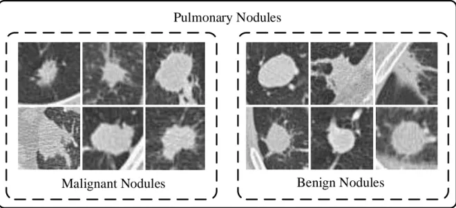
Pulmonary Nodules

Benign Nodules

Malignant Nodules

Figure 3.1: Visual representations of the pulmonary nodule patches in axial view. The pulmonary nodules consists of two main categories: benign and malignant nodule. The nodule images are captured under LUNGx database [26].

to transform representations of input features, ConvNets can learn and extract numerous amount of high-level discriminative features from the raw image at multiple levels of abstrac-tion while whole networks are trained in a supervised manner to perform classificaabstrac-tion due to similar output structure of ANNs. As a consequence, the characteristics of ConvNet are well suited to pulmonary nodule detection when low-level features always resulted in inaccurate prediction and entire classification process should be done in an automatic fashion.

3.3.1 Shallow ConvNet

Early attempts have made to overcome classification of the lung disease patterns via Con-vNets. A shallow ConvNet was proposed to classify patch-based images with interstitial lung disease (ILD) [36]. Like pulmonary nodule patterns as illustrated in Figure 3.1, ILD pat-terns also have high variation texture within the same class while different classes often have similar visual representation. The previous ConvNet [36] showed the remarkable capability of extraction on high-level discriminative features in comparisons of LBP, SIFT, and RBM. However, the previous ConvNet, using single convolutional layer, captures high-level features insufficiently because such shallow structure cannot demonstrate the full potential of feature

(35)

Input Image

32×32

Conv/ReLU

Conv input depth: 1 Conv output depth: 12

Filter size: 7×7

Pooling

Pool input depth: 16 Pool output depth: 16

FC # of hidden neurons: 100 FC # of hidden neurons: 50 FC/SoftMax # of hidden neurons: 2 Pooling FC FC/SoftMax Conv/ReLU Input Image FC

Figure 3.2: Schematic of the Shallow ConvNet [36]. Conv/ReLU, convolutional layer followed by rectified linear unit; pooling, maximum pooling layer; FC, fully-connected layer; FC/SoftMax, fully-connected layer followed by SoftMax.

extraction based on the hierarchy of abstraction which usually requires a deeper structure. The schematic of the Shallow ConvNet is shown in Figure 3.2.

3.3.2 ConvNet with Two Convolutional Layers

In contrast with the shallow ConvNet [36], Song et al. [55] adopted a deep ConvNet struc-ture with two convolutional layers (as shown in Figure 3.3). The ConvNet [55] achieved statically higher precision on malignancy detection of the pulmonary nodule compared to ANN and Stacked Autoencoder [64] which is a neural network based unsupervised learning algorithm. The architecture of ANN and SAE mainly consists of fully-connected layers, so such an architecture with fully-connectives in-between hidden layers always fail to analyze invariant features within the local region, and the pulmonary nodule patterns are usually

(36)

Input Image

28×28

Conv/ReLU

Filter size: 5×5

Pooling

FC

# of hidden neurons: 512

FC/SoftMax

# of hidden neurons: 2

Conv/ReLU

Filter size: 5×5

Pooling

Pooling FC Conv/ReLUPooling FC/SoftMax Conv/ReLU Input Image

Figure 3.3: Schematic of the ConvNet with two convolutional layers [55]. Conv/ReLU, convolutional layer followed by rectified linear unit; pooling, maximum pooling layer; FC, fully-connected layer; FC/SoftMax, fully-connected layer followed by SoftMax.

highly correlated in-between benign and malignant nodule.

3.3.3 ConvNet with Two Grouped Convolutional Layers

A grouped convolution based ConvNet was proposed to detect pulmonary nodule [37]. The grouped convolution was initially introduced in AlexNet model [33] to reduce computation costs when the output depth of convolutional layer is deep. Grouped convolution also im-proves classification accuracy when a deep convolutional layer divides into a group of two light convolutional layer [67]. As shown in Figure 3.4, the grouped ConvNet has two groups of two convolutional layers in a series.

(37)

3.3.4 ConvNet with Three Convolutional Layers

Another recent successful CAD system for malignancy detection of the pulmonary nodule employs three successive convolutional layers [68]. After trained with 1,018 real clinical pulmonary nodules, the trained model achieved diagnosis on malignancy detection of the pulmonary nodule as well as a real radiologist. Figure 3.5 shows the architecture of the ConvNet with three convolutional layers.

3.3.5 Transfer Learning on AlexNet

Instead of training ConvNet model from scratch, using the pre-trained model to train new data has demonstrated nonperformance in the classification of medical image tasks [6, 63]. Training pre-trained weights to adopt new data is defined as progress of transfer learning. Transfer learning reduces risks of over-fitting and issue of convergence. Especially, medi-cal images always have difficulty to optimize clusters of the classifier due to similarities of its features. More recent studies applied pre-trained deeper ConvNet (AlexNet [33]) with transfer learning to classify pulmonary embolism patterns [58]. The AlexNet consists of 5 convolutional layers, and the architecture of the AlexNet is shown in Figure 3.6. By applying transfer learning, the AlexNet inherited capability of feature extraction from the pre-trained model which had shown state-of-the-art performance on the natural image. However, doubt has raised between transfer learning and customized architecture regarding the significant differences between natural images and medical images.

(38)

Input Image

32×32

Conv

Conv input depth: 1 Conv output depth: 8 Filter size: 5×5

Conv

Pooling

Conv

Filter size: 5×5

Pooling

Conv

Filter size: 5×5

Pooling

FC # of hidden neurons: 150 FC # of hidden neurons: 50 FC # of hidden neurons: 100 FC/SoftMax # of hidden neurons: 2 Pooling FC Conv/ReLU Pooling FC/SoftMax Conv/ReLU Input Image Pooling Conv/ReLU Pooling Conv/ReLU FC

Figure 3.4: Schematic of the ConvNet with two grouped convolutional layers [37]. Conv/ReLU, convolutional layer followed by rectified linear unit; pooling, maximum pooling layer; FC, fully-connected layer; FC/SoftMax, fully-connected layer followed by SoftMax.

(39)

Input Image

50×50

Conv

Filter size: 7×7

Pooling

Conv

Filter size: 7×7

Pooling

Conv

Filter size: 7×7

Pooling

Conv/ReLU/SoftMax

Filter size: 1×1 Pooling Conv Pooling Conv Input Image Conv Pooling Conv/ReLu/ SoftMax

Figure 3.5: Schematic of the ConvNet with three convolutional layers [68]. Conv, convolutional layer; pooling, maximum pooling layer; FC, fully-connected layer; Conv/ReLU/SoftMax, convolutional layer followed by rectified linear unit and Soft-Max.

(40)

Input Image

227×227×3

Conv/ReLU/Norm

Filter size: 11×11

Pooling

Conv

Pooling

Conv/ReLU/Norm

Filter size: 5×5

Pooling

Conv

Conv input depth: 384 Conv output depth: 256 Filter size: 3×3 FC/Dropout # of hidden neurons: 4096 FC/Dropout # of hidden neurons: 4096 FC/SoftMax # of hidden neurons: 2 PoolingConv/ReLU/Norm Pooling Conv/ReLU/Norm Input Image

Conv Conv Conv FC/Dropout

FC/SoftMax FC/Dropout

Figure 3.6: Schematic of the AlexNet [33]. Conv/ReLU/Norm, convolutional layer fol-lowed by rectified linear unit and batch normalization; pooling, maximum pooling layer; FC/Dropout, fully-connected layer followed by dropout; FC/SoftMax, fully-connected layer followed by SoftMax.

(41)

Chapter 4 Proposed Method

This chapter aims to provide the detailed definition of the proposed CAD system. Flowchart of the proposed CAD system is shown in Figure 4.1(a). The proposed CAD system is a novel patch-based malignancy detection tool to learn and capture high-level discriminative features of the pulmonary nodule in a supervised manner and learned features are used for nodule diagnosis without any additional classifier. The system consists of two main stages as fol-lows: 1) data preparation aims to provide ROIs in conditions of spatial transformations. 2) ConvNet performs feature extraction and classification by taking advantage of more relevant information provided from the first stage.

4.1 Data Preparation

Common CAD systems for pulmonary nodule detection aim to analyze the marked area of concern. Data preparation is an important stage to enhance texture description on the nodule that improves feature extraction in the following stage. The data preparation stage is shown in Figure 4.1(b). The data preparation stage consists of three steps: 1) extract ROIs from CT images. 2) over-sampling ROIs. 3) contrast normalization.

The extracted ROI presents the pulmonary nodule as a 2-D image patch, and the image patch highlights the pulmonary nodule within a relatively large region compared to the normal CT slice image. Because it is common that medical imaging database usually has limited data size in contrast of natural imaging database, extracted ROIs are over-sampled via spatial transformation, so the increased number of training samples reduce the risk of over-fitting. On the other hand, different CT scanners lead various changes in illumination of the CT slice image. The contrast normalization is used to reduce the illumination effect by

(42)

Axial plane Sagittal plane Extract ROIs 90◦ 180◦ 270◦ Data Augmentation Contrast Normalization Global mean

of intensities Normalized image

Augmented image patch

−

Extracted ROI Augmented image patches

(b) Feature Extraction Classification ConvNet LUNGx Database Extract ROIs Data Augmentation Contrast Normalization Data Preparation Malignant Nodule Detection (a) A patient CT scan Extracted ROIs Subtraction Conv/ReLU Pooling “Malignant” FC/Dropout “Benign” Class scores Feature Extraction Feature Classification (c) Normalized image Conv/ReLU PoolingConv/ReLU Pooling FC/SoftMax

Figure 4.1: Overview of the proposed CAD system. (a) The flowchart of the pro-posed CAD system. (b) Illustration of the data preparation stage. (c) Schematic of the ConvNet. Conv/ReLU, convolutional layer followed by rectified linear unit; pool-ing, maximum pooling layer; FC/Dropout, fully-connected layer followed by dropout; FC/SoftMax, fully-connected layer followed by SoftMax; ConvNet, Convolutional neu-ral network.

(43)

normalizing the intensities of the ROIs. In the following sections, the detailed method of ROI extraction is described in section 4.1.1, followed by the data argumentation (section 4.1.2) and contrast normalization (section 4.1.3).

4.1.1 ROI Extraction

The proposed CAD system extracts ROIs in the axial plane, and the extracted ROIs con-tain the full size of the pulmonary nodules. Typical ROI extraction is done by a manual segmentation [2, 41] or automatic detection via the CAD systems [27, 44, 45]. Since LUNGx Challenge database has already provided approximated central mass of each confirmed nod-ule, ROIs are manually extracted by cropping the axial CT images with bounding boxes. Such bounding boxes have fixed cropping size for each nodule, depending on the visual size of the nodule while keeping the same aspect ratio to prevent information loss when rescaling to match input size of the proposed ConvNet.

Samples of bounding boxes with representations of nodules are shown in Figure 4.2(a) and Figure 4.2(c), and the extracted ROIs demonstrate that the sizes of the pulmonary nodules maintain the major portion of the image patch. If the presence of the pulmonary nodule is in a small region of the ROI, the feature information obtained by the ConvNet is not enough to determine whether there is a pulmonary nodule in the input image patch due to the ConvNet extracts image features within numerous local regions. This can also lead to the decrease in classification accuracy. In addition to the architecture of the proposed ConvNet (as described in section 4.2), three maximum pooling layers are employed to reduce redundant local features by sub-sampling the input feature maps. Therefore, if the size of the pulmonary is too small to be recognized in the ROI, the presence of the pulmonary nodule in the feature maps located in-between the last pooling layer and the first FC layer is too small to provide enough information.

In terms of the ROI size, extracted ROIs are resized to 64×64 pixels to match the input

size of the proposed ConvNet. From the practice of the ConvNet, the ConvNet which has relatively large input size requires a lot more parameters to process the input images. With too many learnable parameters, the classification performance of the ConvNet is degraded because of over-fitting. Also, each ROI is extracted in the axial plane which represents

(44)

a cross-sectional slice of the CT scan, so each nodule generates various numbers of ROIs, depending on the size of the nodule volume. The samples of the ROIs extracted from single benign and malignant nodules are illustrated in Figure 4.2(b) and Figure 4.2(d).

(a)

(c)

(b)

(d)

Figure 4.2: Extracted ROIs from LUNGx Challenge database [26]. Images (a) and (c) show the bounding boxes of the pulmonary nodules. Image (a) shows a malignant nodule from 68-year-old female. Image (b) shows extracted ROIs from the malignant nodule. Image (c) shows a 79-year-old female with benign nodule. Image (d) shows samples of the extracted ROIs from the benign nodule.

4.1.2 Data Augmentation

To achieve promising classification results for the diagnosis of the malignant pulmonary nodule, ConvNets rely on massive numbers of learned parameters. However, deep structures always increase the chance of over-fitting when dataset used to train is limited. Because

(45)

limited training dataset misleads learned parameters to achieve local optima, the correct prediction only occurs when input data is very close or exact as training dataset. To reduce the risk of over-fitting, data augmentation is used to generate spatial invariance on extracted ROIs. Natural images usually contain geometrical information. For example, an image of the residential house consists of the high-level geometrical structure such as the sky. By applying spatial transformation such as rotation or flipping, the transformed natural image fails to demonstrate the geometrical information. In contrast of natural images, geometrical information is trivial to describe nodule. It is still valid to present nodule in any orientation. In this thesis, each extracted ROI is over-sampled to 3 additional artificial image patches by rotating 90, 180 and 270 degrees.

4.1.3 Contrast Normalization

After rotation transformation, contrast normalization is applied to augmented image patches. By subtracting the global average of intensities which is computed from the entire dataset, the augmented image patches achieves zero-centering, and the zero-centering refers to the zero mean of the entire dataset. Thus, the normalized image has fewer sensitives for illumination changes which usually happened when a CT examination is taken on different CT scanner.

For example, a dataset consists of n image patches, and each image presents as an image

tensorxi,j in the spatial domain, so the global mean of the entire dataset (x) can be expressed

as: x= 1 n X i,j xi,j (4.1)

Contrast normalization also improves performance and reduce training time [29]. Because the learnable parameters are optimized by gradient descent algorithm, normalized images have less spatial variance due to zero-centering, so the contrast normalization avoids steeper gradient update which can significantly affect the training performance because a steeper gradient leads a larger number of update in learning parameters. Hence, the training without contrast normalization has the higher risk to miss the global minima of the loss function, and the trained model is easy to over-fitting.

Convolutional Neural Network based Malignancy Detection of Pulmonary Nodule on Computer Tomography