Fermilab
FERMILAB-THESIS-2000-10CDF/THESIS/JET/PUBLIC/5555
Version 1.0
12th February 2001
Calorimetric Measurements in CDF:
A New Algorithm to Improve
The Energy Resolution of Hadronic Jets
A Thesis Submitted
to
the University of Cassino
by
Giuseppe Latino
in Candidacy for the Degree
of
Doctor of Philosophy
Cassino, ITALY
Abstract
Many interesting physics signatures in a collider experiment like CDF are characterized by nal state quarks and gluons which fragment into hadronic jets. An improvement in the jet energy resolution is then very important for many Run II physics analyses and any eort in pursuing such result can be rightly considered as part of the complex CDF II upgrade program.
The jet energy resolution comes from many sources, which can be grouped into two categories: detector and physics eects. In the work exposed in this thesis, detector eects were extensively treated developing a new algorithm which allows to optimize the jet energy resolution using calorimetry as well as additional detector information. For the rst time in a hadron collider the full granularity of the detector was adopted to perform corrections at \tower level" rather than at the usual \jet level", this allowing the new algorithm to be exploited regardless of the clustering algorithm chosen to reconstruct the jet.
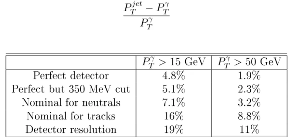
In the present work the new algorithm has been optimized and imple-mented in an oine code which in principle allows it to be applied on each data sample. A preliminary study on potential algorithm improvements was also performed. The algorithm test, as performed on two dierent Run Ib data samples, -jet and di-jet, showed very promising results up to 25%
Ph.D Thesis
Calorimetric Measurements in CDF:
A New Algorithm to Improve
The Energy Resolution of Hadronic Jets
Giuseppe Latino
ADVISORS:Prof.
Giovanni Maria Piacentino
(University of Cassino)
Prof.
Stefano Lami
Contents
Introduction
4
1 CDF at Fermilab
6
1.1 Hadron colliders . . . 6 1.2 The Tevatron . . . 8 1.3 The CDF II Detector . . . 11 1.3.1 Tracking System . . . 13 1.3.2 Calorimetric System . . . 20 1.3.3 Muon System . . . 22 1.3.4 Trigger System . . . 22 1.4 The CDF I Detector . . . 23 1.4.1 Tracking . . . 23 1.4.2 Calorimetry . . . 24 1.4.3 Trigger . . . 262 Jets at CDF
27
2.1 Jet Reconstruction . . . 272.1.1 CDF Jet Clustering Algorithm . . . 29
2.1.2 Jet Energy and Momentum Reconstruction . . . 30
2.2 Jet Energy Corrections . . . 30
2.2.1 JTC96 Jet Corrections . . . 31
2.2.2 Uncertainties in Energy Scale . . . 36
2.2.3 Specic Corrections . . . 36
2.3 Jets in Physics Events . . . 37
2.3.1 The CDF II Physics Program . . . 37
3 A New Jet Correction Algorithm
44
3.1 Introduction . . . 443.2 Preliminary Study With the CDF Simulation . . . 47
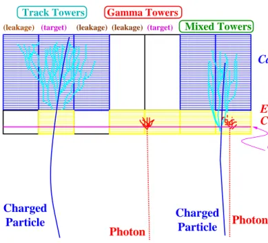
3.3 The Classication Method . . . 49
3.3.1 Track Tower . . . 50 1
CONTENTS
2
3.3.2 Gamma Tower . . . 52
3.3.3 Not Assigned Tower . . . 55
3.3.4 Mixed Tower . . . 55
3.3.5 CES Fake Clusters . . . 56
3.4 Monte Carlo Study of the Classication Method . . . 57
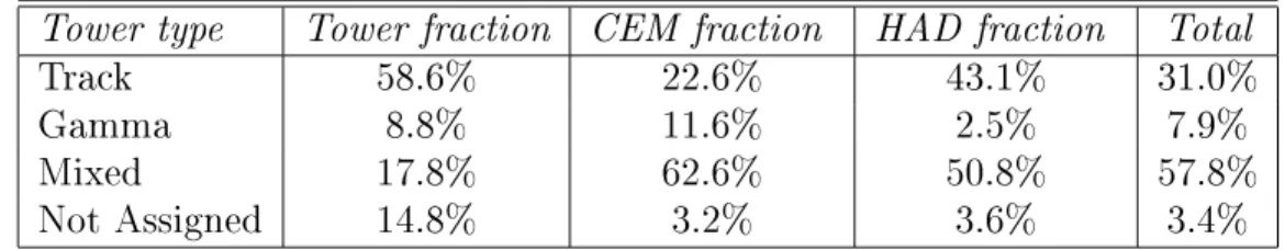
3.5 Incidence of Dierent Classied Towers . . . 59
3.6 The New Denition of Tower Energy . . . 60
3.6.1 Parameter Selection . . . 62
3.7 A New Jet Correction Code: JCOR2K . . . 65
3.7.1 JCOR2K . . . 68
3.8 Future Algorithm Developments . . . 69
4 Testing the New Algorithm
73
4.1 The -jet Sample . . . 734.1.1 Previous Studies . . . 75
4.1.2 Data-Monte Carlo Comparison . . . 77
4.1.3 The Photon Sample Selection . . . 77
4.1.4 Jet Energy Resolution . . . 81
4.1.5 Further Studies . . . 83
4.2 The Di-jet Sample . . . 87
4.2.1 The Di-jet Sample Selection . . . 87
4.2.2 Event Energy Scale . . . 89
4.2.3 Jet Resolution Measurements . . . 91
4.2.4 6~ET Resolution Studies . . . 96
5 Jet Studies With the New Algorithm
98
5.1 A Golden Subsample . . . 985.2 Something Strange . . . 99
5.3 Cosmics Background Studies . . . 101
5.4 Jet Studies . . . 107
A Jets in QCD
116
A.1 The Standard Model . . . 116A.1.1 Fundamental Forces . . . 116
A.1.2 Leptons and Quarks . . . 117
A.2 Hadron Structure and Connement . . . 119
A.2.1 Fragmentation . . . 121
A.3 A brief Jet History . . . 121
A.4 Jet Phenomenology . . . 122
CONTENTS
3
Conclusions
125
Acknowledgements
126
Introduction
The Collider Detector at Fermilab (
CDF
) is a particle detector to study the high mass states and large transverse momentum phenomena produced by the collision of proton and antiproton beams at the Tevatron Collider. The data collected in the period 1992-1996 (Run I) allowed the discovery of the top quark.Run II at the Tevatron Collider will start in March 2001, providing col-lisions with an instantaneous luminosity up to 210
32cm,2s,1 (about one
order of magnitude greater than in Run I) and with a center-of-mass energy increased from 1.8 TeV to 2.0 TeV. The upgrade of the accelerator will con-rm the Fecon-rmilab Tevatron Collider as the high energy frontier of particle physics and put the CDF experiment in the exciting position to improve Run I measurements and search for new physics for many years to come.
The goal of this new run is the accumulation of an integrated luminosity of at least 2 fb,1 at
p
s = 2:0 TeV in the rst two operational years. After that, the Tevatron Collider program will be hopefully extended for other years, with a higher luminosity, so that 20 fb
,1 of data could be collected
before the new Large Hadron Collider at CERN will start running.
The increased luminosity and energy required some modications to the experimental apparatus. Based on ten years of experience with CDF and Tevatron physics, the detector, as described in Chapter 1 , has been upgraded with many new powerful features. Best attention has been also devoted to the performance of both data acquisition and oine analysis.
Many interesting physics signatures in a collider experiment are charac-terized by a quark or a gluon in the nal state. But quarks and gluons cannot be seen as free particles because they are subject to a fragmentation process making them to experimentally appear as hadronic jets. From Run I data analysis, we have experienced that a limited jet energy resolution is the main source of error in many processes. Therefore, an improvement in the jet energy resolution would have a big impact on some of future Run II physics results, like for instance the top quark mass resolution (where the reconstruction of jet energies is involved) and the search for the Higgs boson
Introduction
5
(expected to mainly decay into two jets). Any eort in pursuing it can rightly be seen as part of the CDF II upgrade program.
Dedicated studies have shown that the jet energy resolution comes from many sources, which can be grouped into two categories: detector and physics eects. In the work exposed in this thesis, detector eects are treated de-veloping a new algorithm which allows to optimize the jet energy resolution using calorimetry as well as additional detector informations. For the rst time in a hadron collider, the full granularity of the detector is adopted to perform corrections at \tower level" rather than at the usual \jet level". In such a way the algorithm improvement can in principle be exploited regard-less of the clustering algorithm chosen to reconstruct the jet.
Chapter 2 describes the standard jet reconstruction and energy correc-tion in CDF and the impact on Run II physics of an improved jet energy resolution. Jet theory and physics are addressed in Appendix A.
A new algorithm to improve the jet energy resolution using calorimetry, tracking and Shower Max information is motivated and described in Chap-ter 3. In particular the original contribution of the candidate in optimizing and implementing the algorithm into an oine analysis code is described. Results of a preliminary study on potential algorithm improvements are also shown.
The application of the new jet algorithm on CDF data, as performed by the candidate, is described in the last two chapters. Chapter 4 reports the results of testing the new algorithm code on two dierent Run Ib data samples, -jet and di-jet, showing very promising results up to 25% of
improvement relative to the standard CDF jet corrections. Further jet studies and cross-checks of the new algorithm are shown in the nal Chapter 5.
Chapter 1
CDF at Fermilab
After a brief introduction to the Tevatron Collider, a description of the CDF detector is given in this chapter, with a particular attention to the detector components which are mainly involved in the work exposed in this thesis.
1.1 Hadron colliders
Particle accelerators can be regarded as giant microscopes, the most sophis-ticate tools to peer into the innermost recesses of matter. Their continuous evolution allows High Energy Physics to make astonishing advances in dis-covering and understanding the fundamental particles and forces of Nature, from which the universe is built. The latest of particle accelerator projects are \colliders", based on the principle of colliding particle beams, which is the most economical way to achieve the highest energies.
High energies are needed to probe small distances in the scattering of one particle from another as well as to produce a new particle whose mass can be materialized only if there is enough spare energy available in the center-of-mass frame. The discovery of several physical processes, like the production of heavy quarks and W and Z vector bosons, has been achieved thanks to very energetic interactions between leptons (typically electrons and positrons) or partons (quarks and gluons conned inside the hadrons), with the highest available energy in the center-of-mass of the collision. These collisions can be obtained by sending a particle beam on a xed target or making two particle beams to collide head-on (collider). In the former the high density of the target gives a higher interaction probability, but the center-of-mass energy p
s available to create a new particle scales with the beam energy as
p
s /
p
E, while in the latter p
s / E. So we can understand the great
interest in designing and building bigger and bigger colliders even if the low 6
1.1 Hadron colliders
7
density of the beams gives a lower interaction probability.
Currently dierent kinds of collider are operating in the world: in lep-ton colliders (like LEP at CERN) the collision occurs between electron and positron beams1; hadron colliders use beams of protons and antiprotons (like
Tevatron at Fermilab) or protons and electrons (like HERA in Hamburg). The hadron collider LHC under construction at CERN will provide proton-proton interactions beginning in 2005. The feasibility of a muon-antimuon collider is presently under study.
While in lepton colliders the interaction directly involves the beam par-ticles, in hadron collisions the interaction involves the partons (quarks and gluons) conned inside the hadrons which typically carry only a low fraction of hadron energy2. On the other hand the negligible incidence of
bremsstrah-lung losses allows to obtain higher energies in hadron colliders with respect to lepton ones.
The most important parameters characterizing a collider performance are:
p
s
: the center-of-mass energy of the interacting beam particlesL : the Instantaneous Luminosity
The former is a critical parameter which sets the upper limit to the particle mass which can be created in the collision.
The latter is typically dened as (in the ideal case of relativistic beams com-pletely overlapping) [1]:
L=Bf
0 NpNp
(1.1)
Where B is the number of bunches circulating in the ring for each beam,
Np(Np) is the number of protons (antiprotons) in each bunch,f0 is the single
bunch revolution frequency and is the bunch cross section. The luminosity is related to the number dn=dtof events of a given process (characterized by a cross section ) which are produced in the time unit:
dn=dt=L(t) =) n(T) = Z T
0
Ldt (1.2)
The quantityLint= R
Ldt(called Integrated Luminosity) is a very important
parameter in a collider experiment giving the total number of events n(T)
1The beam particles are actually grouped into bunches so that a collision can be
ob-tained when two opposite bunches overlap.
2At high energies, like at Tevatron, this parton connement inside the hadrons tends
to disappear (Asymptotic Freedom) so that the proton and antiproton beams are actually \parton beams" with a wide momentum band.
1.2 The Tevatron
8
(for the given process) collected during the time T of data taking. From the above: [L] = [cm
,2][sec,1] while typically [
Lint] = [b
,1] where the
barn(b) is the standard unit for nuclear cross section (1b = 10,24 cm2).
1.2 The Tevatron
The Tevatron Collider at Fermi National Accelerator Laboratory (Fermilab), located 50 Km west of Chicago, is a proton-antiproton collider which allows a center-of-mass interaction energy p
s = 2 TeV 3. This energy will be the
highest available in the world until around 2005 when LHC (at CERN) will be operative at p
s= 14 TeV.
The Tevatron is a double acceleration ring with a radius of 1 Km where proton and antiproton bunches circulate in opposite directions bent by su-perconducing magnets. The bunches can collide in two experimental areas, B0 and D0, where the experiments CDF II and D0 are respectively placed. This accelerator is also designed for xed target experiments: 0.8 TeV proton bunches are extracted and sent to other experimental areas [2].
During the last four years this accelerator has been upgraded in order to increase both p
s and L. In particular, the construction of the Main
Injectorand of the Recycler Ring was nalized to increaseL (mainly limited
by the particle density in the antiproton bunches) by increasing the number of bunches circulating in each beam. The new operational period (Run II) is scheduled to begin on March 2001.
The Tevatron is actually the last stage of the accelerator system which is schematically shown in g. 1.1. The dierent parts of this complex are used in successive steps to produce and store the particle bunches sent to the Tevatron. The beam production can be schematically described as follows.
Proton Beam
: H, ions are produced by ionization of gaseoushydro-gen and then accelerated up to an energy of 750 KeV by a Cockroft-Walton electrostatic accelerator. Then they are injected in a 150 m long linear accel-erator (Linac) which increases their energy to 400 MeV. After being focused, theH,ions are made to collide on a thin carbon target and in this interaction
they lost the two electrons becoming protons. The protons are then injected in the Booster, a 75 m radius synchrotron where they reach the energy of 8 GeV and are grouped into bunches each containing up to 510
12 particles.
These bunches are then sent to the Main Injector, a synchrotron accelerating them to 150 GeV. Finally the protons are injected into the Tevatron, a 1 Km radius synchrotron using superconducting magnets producing a eld of 5.7
3In the period 1992-1996 (Run I) this collider was operated at p
s= 1.8 TeV allowing the discovery of the topquark.
1.2 The Tevatron
9
Figure 1.1: Fermilab accelerator complex.
T, where they reach the nal energy of 1 TeV.
The Main Injector is the most important achievement in the Fermilab up-grade program for Run II [2]. It has been designed to solve most of the problems met with Run I when the Main Ring, a conventional synchrotron placed over the Tevatron in the same ring, served as injector. The Main Ring could not accept all protons from the Booster and also it created in-eciencies and backgrounds during the data acquisition from the Tevatron being the two accelerators in the same tunnel. Conversely the Main Injector allows an optimal interconnection between the Booster and the Tevatron: we expect an increase of 50% in protons for each production pulse and of 60% in proton pulse frequency.
Antiproton Beam
: a proton bunch of 120 GeV, extracted from the Main Injector, is sent to a rotating nichel target after being focused. In this collision several nuclear products are generated among which antiprotons with a wide angular and momentum spread. A suitable magnetic eld and a litium magnetic lens allow to select and focus the antiprotons in bunches having 8 Gev in average energy. The antiprotons are then sent to the De-buncher, a storage ring which narrows theirs momentum distribution using the Stocastic Cooling technology. At the same time the particle spatial spread is increased so to reduce the bunches to a continuous beam which is sent to the Accumulator, another storage ring placed inside the Debuncher. Here the1.2 The Tevatron
10
antiprotons are continuously stored during the various Debuncher cycles and subject to further stocastic cooling. This accumulation process continues un-til a current sucient to give 36 (121)4 bunches with acceptably high density
is stored. The antiprotons are then injected into the Main Injector which accelerates them to 150 GeV and nally in the Tevatron where, circulating in opposite direction with respect to the proton bunches previously injected by the Main Injector, they reach the energy of 1 TeV.
After each accumulation-acceleration-interaction cycle when the beams are degraded, the antiprotons still circulating inside the Tevatron are decelerated rst in the Tevatron and then in the Main Injector up to 8 GeV and then sent to the Recycler. This is a Stocastic Cooling Ring placed in the same tunnel of the Main Injector where the antiprotons coming both from the Ac-cumulator and from the Tevatron (through the Main Injector) are stored till a new boosting injection in the Main Injector and then in the Tevatron. In such a way the Recycler, which is able to store up to 510
12 antiprotons,
allows an \antiprotons recycling" resulting in an increased luminosity. In Run IIa (Run IIb), 36 (140) proton bunches and 36 (121) antiproton bunches circulate in opposite directions inside the Tevatron, colliding every 396 (132) ns in the center of the CDF II and D0 detectors. At each bunch crossing the interaction region is characterized by a gaussian spatial distribu-tion withz 16 cm in the beam direction andt 16m in the transversal
one.
The increase in the number of beam bunches with respect to Run I (6 bunches per beam) allows to increase the luminosity reducing at the same time the bunch particle density which results in a lower average interaction number in each bunch crossing and so in \cleaner" physical events. The Fermilab Accelerator Complex upgrade is expected to allow the Tevatron to deliver an instantaneous luminosity of 210
32cm,2sec,1 which will provide 2fb,1 of
integrated luminosity at p
s= 2 TeV after 2 years of data acquisition [2]. On the other hand the reduced time between two bunch crossing (3500 ns
in Run I) and the increase in the collision energy have inuenced most of the CDF Detector upgrade program: from the choice of the active part of new subsystems to the design of the new readout electronics.
Table 1.1 reports the most important beam parameters for the dierent Teva-tron operating congurations [2].
4These two numbers are related to the two dierent operative congurations planned
for the Tevatron: 36 antiproton bunches for a beams interaction every 396 ns (Run IIa), 121 for a beams interaction every 132 ns (Run IIb).
1.3 The CDF II Detector
11
Run Run Ib Run IIa Run IIb # of bunches (pp) 66 3636 140121 pper bunch 2:310 11 2:7 10 11 2:3 10 11 pper bunch 610 10 7 10 10 7 10 10 p rms bunch length (cm) 63 37 37 p rms bunch length (cm) 59 37 37 Beam energy (GeV) 900 1000 1000
Bunch spacing (ns) 3500 396 132 Luminosity (cm,2sec,1) 1:6 10 31 >5 10 31 2 10 32 Interactions/collision average # 2.5 2.3 1.3
Table 1.1: Comparison among the most important beam parameters for the dif-ferent Tevatron operating congurations. Run Ib was the last period of data ac-quisition of the previous run (1994-96). Run IIa is scheduled to start March 2001 while Run IIb after the rst two operative years of the new Tevatron.
1.3 The CDF II Detector
The Collider Detector at Fermilab (
CDF
) [3, 4, 5] is a collection of detec-tion devices designed to study a wide range of physical processes produced in proton-antiproton collisions and characterized by nal state particles with high transverse momentum. This equipment is nalized to detect photons, electrons, muons, hadronic jets and (indirectly) neutrinos, measuring their position, energy and momentum. In order to achieve these goals and con-sidering the energy equivalence of the two beams, it is characterized by an almost complete coverage in solid angle and by an azimuthal and \back-forward" symmetry with respect to the nominal interaction point.CDF is a general purpose detector. With the accelerator providing up to about 7.6 million collisions per second, it can pick up online just the most interesting events according to several dierent physics programs. The rst version of the CDF detector collected data starting 1987. During Run I (1992-96) the CDF collaboration achieved very important physics results: the discovery of the topquark [6], precision measurement of the W mass [7], the
preliminary measurement of sin2 [8] and the discovery of theBcmeson [9].
In the last four years the CDF detector underwent a major upgrade with the addition of almost a million new detector elements that will allow CDF to make even more precise measurements and search for new phenomena for many years to come. The
CDF II
detector will be able to cope with the new Tevatron operative conditions (increase in collision energy and fre-quency) and to overcome some detector limitation seen during Run I (track1.3 The CDF II Detector
12
reconstruction, muon detection, forward calorimetry).
CDF adopts two coordinate systems according to the following conven-tion: cartesian coordinates (x;y;z) with origin in the nominal interaction point, z axis along the beam direction according the proton motion, x axis going outside the Tevatron ring andyaxis up perpendicular to the ring plane; polar coordinates(r;;) oriented according to the usual convention with re-spect to the cartesian ones. Like other collider experiments the following variables are very often used: the pseudorapidity which is related to the polar angle by
= ,log[tan(
2)] (1.3)
and the projection on the transverse plane of the particle energy and mo-mentum, ET =Esin and PT =P sin.
The whole detector system is composed of three regions: the central one covering therangejj1 and the two plug ones which symmetrically cover
the \backward" and \forward" regions with 1jj3:6. Starting from the
nominal interaction point the central detector can be divided into three main substructures:
Tracking System Calorimetric System Muon System
The two plug detectors are essentially calorimetric and muon systems being an extension up to jj3:6 of the corresponding central systems.
Finally the Trigger System allow to select the rare physical events of in-terest to be written on tape with a drastically reduced rate respect to the bunch crossing one.
As the work exposed in this thesis is part of the CDF upgrade program, the CDF II upgraded system will be described in this section. Nevertheless, as both simulation and data sample were used relatively to Run I, a brief description of CDF I will be also given in next section.
Given the complexity of the CDF apparatus, only a general description is provided, with a particular emphasis to the detector components mostly involved in the work of the present thesis. The main detector structures are sketched in g. 1.2.
1.3 The CDF II Detector
13
Figure 1.2: Side view of the CDF II detector.
1.3.1 Tracking System
This system is placed inside a 4.8 m long and 3 m wide superconducting solenoid, which provides an uniform magnetic eld parallel to the beam axis of about 1.4 Tesla. It allows a 3-D track reconstruction for charged parti-cles traversing the eld region and so, by track deection, to measure their charge and transverse momentum. It consists of a microstrip silicon sec-tion (L00+SVXII+ISL), which gives a precise tracking around the beam, surrounded by a cylindrical drift chamber (COT).
Layer00
The Layer00 (
L00
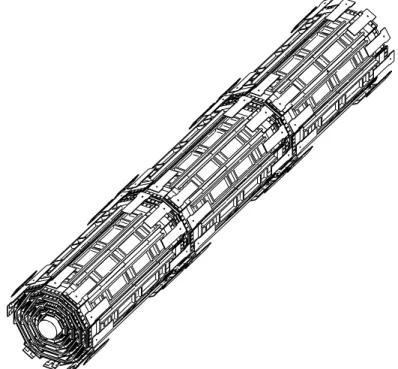
) is a vertex silicon detector placed just outside the beril-lium beam pipe at 1.6 cm from the beam axis [10]. It is made by a layer of single sided microstrip silicon detectors parallel to the beam giving track information in the r- plane. Fig. 1.3 shows one of the two parts constitut-ing this device. A new technology allows to polarize these sensors to high voltage (500 V) which gives a good signal-to-noise ratio (S/N) even after1.3 The CDF II Detector
14
Figure 1.3: Drawing of one half of L00. Four sensor groups (blue) starting at z = 0 and the readout hybrids (magenta) starting at z45 cm are shown. The cooling
system is shown in red.
the beam pipe for about 80 cm, have a strip separation of 25 m and a 50
m readout pitch. This allows a 6 m single point resolution in the trans-verse plane. To reduce the radiation damage eects the sensors need to be operated at about 0 oC, which requires a cooling system embedded in their
carbon ber support. The readout electronics is placed in a separate zone to avoid both silicon heating and radiation damage problems and is connected to the about 16,000 channels by special cables. Detector signals are processed by the SVX3D chips which are the same, like the combined data acquisition system, used for all the silicon tracking system.
SVXII
Outside the L00, between 2.4 and 10.6 cm from the beam axis, ve double sided microstrip silicon layers are placed which constitute the Silicon VerteX Detector II (
SVXII
) [5]. Three of them allow to get the track position on the r- plane from the readout of one side (microstrips parallel to the beam axis) while the z coordinate is read from the other side (microstrips perpendicular to the beam axis). The other two layers give track information on r- from one side and r-0 from the other, having the microstrips tilted1.3 The CDF II Detector
15
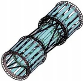
Figure 1.4: Final SVXII assembly with the silicon detectors mounted on the three barrels.
of 1.2o in a stereo conguration respect to the z axis5. In such a way it is
possible to have a 3-D track reconstruction with an approximatively uniform eciency. The strip pitch is 60 m on the r- readout side while is varying from 60 to 140m on the r-0 and z one. This detector has been designed to
give (with an improved coverage of the pseudorapidity region) a 3-D vertex reconstruction and to provide track information up tojj2 with an impact
parameter resolution<30m andz<60m for central high momentum
tracks. The sensors are mounted on three mechanical structures (barrels) covering a total length of 96 cm along the z coordinate and are segmented into 12 wedges in . The barrels also support the water cooling channels for the readout electronics. Fig. 1.4 gives a sketch of the complete barrels assembly. The almost 406,000 channels of SVXII are read by the readout chips SVX3D placed on its external sides along z. Both SVX3D chips and SVXII detectors are designed and tested to be \radiation-hard" considering the strong radiation eld in which they have to operate. We expect that after about 3 fb,1 of integrated luminosity the two innermost layers (Layer0
and Layer1) will have a signicant worsening, but the additional information from Layer00 will allow good inner tracking up to 5 fb
,1.
5This sensors with one side 1.2otilted strips are obtained from new 6 inch silicon wafers
1.3 The CDF II Detector
16
Intermediate Silicon Layers
The Intermediate Silicon Layers Detector (
ISL
) is a charged particle detec-tor placed in the radial intermediate region between SVXII and the central tracking system (COT) [5]. Fig. 1.5 shows the position of the ISL silicon layers. They are in the radial range 20 < r < 30 cm extending to jzj =65 cm for the inner layer and jzj = 87.5 cm for the outer one and covering
an overall pseudorapidity zone up to jj 2. For jj 1, where the COT
tracking information is more complete, ISL is made by a single detector layer at r = 22 cm; for 1jj2 two layers are placed atr = 22 and 28 cm.
Figure 1.5: Positions of all the silicon layers constituting the inner silicon tracker system. The pseudorapidity coverage regions are also shown. The z scale has been compressed.
Figure 1.6: Overall ISL assembly. The readout modules are installed on a carbon ber structure also containing the SVXII detector.
1.3 The CDF II Detector
17
The total ISL extension in z is about 2 m for an overall silicon active surface of about 3.5 m2. The azimuthal segmentation into \wedges" is such
that a complete coverage is obtained without ineciencies. The overall ISL assembly is shown in g. 1.6.
The microstrip silicon crystals used in ISL (58mm76mm) are the same
as SVXII and are double-sided with axial strips on one side and small angle (1:2o) stereo strips on the other. The microbounding of 3 crystals connected
to their readout electronics (same SVX3D chips as SVXII) gives a ladder which is the basic electric readout unit . ISL has 296 of such ladders for a total of about 300,000 readout channels connected to the data acquisition.
In principle a charged particle, before entering the COT, leaves 13 mea-surement points in the inner silicon system (L00+SVXII+ISL). So this three detector can be considered an independent tracking system forjj2 giving
a 3-D track reconstruction. As consequence tracking, lepton identication and b-tagging capabilities can be extended over this full region. Moreover an improvement in the overall track t is attended in the central region where the ISL will provide a further measurement point between the SVXII and the COT. From preliminary simulations [5]: the single hit resolution is expected to be 20m in the transverse plane; the impact parameter resolution is
expected to be d 15m while for the transverse momentum resolution
PT
PT
0:4%PT. A 8% fake track incidence is nally expected.
Central Outer Tracker
Forjj1, tracking at large radii is performed by the Central Outer Tacker
(
COT
), a large cylindrical open cell drift chamber [5], which substituted the old drift chamber (CTC) used in Run I. This device is 3 m long occupying the radial range 44 < r < 132 cm (see g. 1.7). The COT is designed to operate with a maximum drift time of 100 ns by reducing the maximum drift distance (obtained with a reduced cell dimension) and by using a gas mixture (50 : 35 : 15 Ar ,Et,CF4) with a faster drift velocity (
100m=ns)
6.
Considering a bunch crossing every 132 ns as operative limit for Run II, this avoids dead times and also allows to use the COT information for the level 1 trigger.
The COT is made by 96 wire coaxial layers. They are grouped into 8 cell superlayers. Four, with wires parallel to the beam axis, giving the
r, coordinate and four giving the z coordinate with a stereo (3o) wire
conguration. A 3-D track reconstruction is so possible. Each basic drift cell contains 12 sense wires alternating with shaper wires. The drift electric eld
6The 706 ns CTC maximum drift time was the fundamental reason for it to be
1.3 The CDF II Detector
18
is 2.5 kV/cm which, for the CDF II central magnetic eld, gives a Lorentz deection angle of 35o 7.
Figure 1.7: Cross view of one half of the COT.
The cell geometry is sketched in g 1.8. Its electrostatic eld conguration is given by a cathode (\eld panel"), which is made by gold on a 0.25 mm thick Mylar sheet, and by wires attached on Mylar strips (\shaper panel") which close both electrically and mechanically the ends of each cell. In such a way the loss eect due to a broken wire is minimized as contained within one cell. Between the eld panels, sense wires alternate in a plane with potential wires. Both are 1.6 mm gold-plated tungsten wires. Signals from the about 30,000 COT readout channels are processed (discriminated, shaped and amplied) and sent to a TDC. Finally they are sent in parallel to the trigger and data acquisition systems.
The COT measurement precision is strongly related to the geometry reg-ularity and to the electrostastic eld uniformity. The single hit resolution is expected to be 180m in the transverse plane while the transverse
mo-mentum resolution is expected PT
PT
0:3%PT. These resolutions are quite
similar to those obtained with the CTC in Run I.
7The Lorentz angle is the deection angle of the drift particles with respect to the
electric eld direction which is due to the solenoid magnetic eld. To get an uniform readout the cells are tilted by this angle respect to the radial direction.
1.3 The CDF II Detector
19
SL2 52 54 56 58 60 62 64 66 R Potential wires Sense wires Shaper wires Bare MylarGold on Mylar (Field Panel)
R (cm)
Figure 1.8: r, view of a single COT cell.
Figure 1.9: TOF scintillator bars in CDF II.
Time of Flight Detector
The Time of Flight (
TOF
) scintillating bars [10] are placed between the COT and the superconducting solenoid cryostat arranged in a cylinder structure. Each of the 216 bars is 2.8 m long and is placed at a radial distance of 138 cm from the beam axis parallel to it (see g. 1.9). Two PMTs read the light from both the bar ends. The TOF measures the times between the bunch crossing1.3 The CDF II Detector
20
and the signals produced into its scintillators by the particles originated in the collision. The particle speed is evaluated by this time and combining this information with the momentum from the tracking system its mass is measured.
Fast precision electronics is used for the time of ight measurements which is expected to give a time resolution of 100 ps on single particle. A 1
separation between and K with P <2:2 GeV/c is expected.
1.3.2 Calorimetric System
Outside the solenoid coil, sampling calorimeters cover the pseudorapidity region jj 3.6 and the entire 2 azimuthal angle [5]. Dierent size and
thickness plastic scintillator and absorber layers are alternatively stacked forming the electromagnetic calorimeters (allowing the energy measurement for photons and electrons) and the hadronic calorimeters (measuring hadron particle energies). The primary particle produces a shower of secondary par-ticles inside the absorber. The shower parpar-ticles deposit a fraction of their energy in the sampling material producing a light signal read by photomul-tipliers (PMTs) through wavelength shifting (WLS) light guides or optical bers. The original particle energy is then obtained with a calibration based on test beam data.
The calorimetric system is composed of two sub-systems: the central calorimeter and the plug calorimeter. Both of them are segmented in the
andcoordinates in order to have a projective tower geometry pointing back to the nominal interaction point (see g. 1.2 and g. 1.10).
In each tower the electromagnetic compartment is backed by the hadronic one, both readout by dierent PMTs. A comparison of electromagnetic and hadronic energy can be made on a tower-by-tower basis allowing the distinc-tion between photons/electrons and hadrons. The tower segmentadistinc-tion also gives a measure the angle at which the particle emerged from the interaction point.
The central calorimeter will be described in next section being the same as in Run I. Here we describe the new plug calorimeter replacing the old plug and forward gas calorimeters no more compatible with the crossing rates for Run II.
Plug Calorimeter
The calorimetric coverage in the backward/forward region (1 jj 3:6)
is provided by two identical
Plug
Calorimeters [5] (see g. 1.10). Both the electromagnetic (EM) and hadronic (HAD) sections of this new calorimeter1.3 The CDF II Detector
21
are sampling devices having scintillator tiles as active elements read out by WLS optical bers embedded in the scintillator. The WLS bers are spliced to clear bers carrying the light out to PMTs placed on the back plane of each endplug. Active and absorber elements are arranged in a tower geometry, common to both EM and HAD sections, whose segmentation varies
with from 0.17:5o to 0.615o.
The EM calorimeter is composed of 23 layers for a total thickness of about 21 X0 (corresponding to
1
0)
8 at normal incidence. Each layer
is composed of 4.5 mm lead and 4 mm scintillator. The scintillator tiles of the rst layer are made out of 10 mm thick scintillator and are read by multi-anode photomultipliers (MAPMTs). They will be used as a Preshower Detector. A Shower Max Detector is also located at the deep of maximum shower development (approximately 6 X0). This position detector is made
of scintillator strips read out by WLS bers carrying the light to MAPMTs. This device will improve the e-/0 separation. From test beam data [11],
the energy resolution of the EM section results 15:5%= p
E1%
9.
Figure 1.10: r-z view of the upper part of the new CDF II plug calorimeter.
8The radiation lengthX
0and the nuclear interaction length 0 of a given material are
respectively dened as the mean distance over which a high-energy electron loses about 1/e of its energy by bremsstrahlung and the mean free path for a hadron (usually a+) to
undergo a nuclear inelastic interaction. They are the appropriate scale length to describe high-energy electromagnetic and hadronic showers, respectively.
9Here and in the following, the symbol
1.3 The CDF II Detector
22
The HAD calorimeter is a 23 layer sampling device with an unit layer made of 5 mm iron and 6 mm scintillator. The overall thickness for a normal incidence is 7
0 and the energy resolution for pions is estimated to be
78%=
p
E5% from test beam data [11].
1.3.3 Muon System
The muon detection will be provided, in the pseudorapidity range jj2:0,
by four systems of scintillators and proportional chambers integrating and extending the old muon system [5]. The muon candidatezand coordinates are provided by the chambers while the scintillator detectors are used for triggering and spurious signals rejection. The calorimeter steel, the magnet return yoke, additional steel walls and the RunI forward muon toroids act as hadron absorber for this system, drastically reducing the \punch-through" incidence.
In the central region (jj0:6) the
CMU
chambers are placed atr 3:5m just outside the calorimeter while at r 5 m, behind a 60 cm iron wall,
there are the
CMP
chambers with an external scintillator layer. At the same radial distance the 0:6jj1:0 range is covered by theCMX
chambers,provided with a double scintillator coverage. Finally the
IMU
chambers, also integrated with scintillators, give muon detection in the range 1:0jj2:0.1.3.4 Trigger System
In Run II operative conditions the Tevatron will provide a bunch crossing rate up to 7.6 MHz while physical events can be written to magnetic tape with
a.50 Hz rate [5]. So a tiered \deadtimeless" trigger system (implemented in
a complex hardware-software architecture) is used to properly select the rare physical processes of interest. Each event is considered sequentially at three levels of approximation with each level providing a rate reduction sucient for the next level to have minimal deadtime.
Like the data acquisition system (DAQ), the trigger is fully pipelined with the Level-1 and 2 using a custom hardware on a limited subset of the data while the Level-3 using a processor farm running on the full event readout. This system is very exible allowing to accommodate over 100 separate trig-ger selections. With a 40 kHz Level-1 accept rate and a 300 Hz rate out of Level-2 a deatime <10% is expected at full luminosity.
A detailed description of the main trigger selection criteria is not possi-ble at the moment as they are not yet completely dened. Here we briey describe the main improvements with respect to the corresponding CDF I system. The track nding (previously available only at Level-2) is added to
1.4 The CDF I Detector
23
Level-1 allowing an improved electron an muon identication. At Level-2 the Silicon Vertex Tracker (SVT) provides the trigger on tracks with large impact parameters, very important to select events with b quarks in the nal state which characterize a large number of interesting processes. At the same time an improved Level-2 track momentum resolution and electron/photon and muon identication will be achieved.
1.4 The CDF I Detector
As shown in the next chapters, the work exposed in this thesis was performed using both simulation and data samples relative to Run I. A brief description of CDF I is then needed regarding the detector components directly involved in this study: tracking, central calorimetry and trigger system.
1.4.1 Tracking
The CDF I tracking system consisted of three separate tracking devices placed inside the solenoid magnetic eld [6].
Outside the 1.9 cm radius beryllium beampipe was a four layer Silicon Mi-crostrip Vertex Detector (
SVX
) consisting of two identical cylindrical mod-ules for a total length of 51 cm and a complete azimuthal coverage up tojj 1:9. Each module was made of 12 wedges consisting of four silicon
detector layers placed at a radial distance ranging from 3 cm to 7.9 cm. This device provided track informations on the transverse plane with a single-hit resolution, measured on data, 13 m and an impact parameter
resolu-tion measured to be d 17m. Its performance resulted to be critical for
the quark top discovery.
Surrounding the SVX, a Vertex Drift Chamber (
VTX
) provided tracking information up tor= 22 cm andjj3:25 also measuring theppinteractionvertex along thez axis with a resolution of 1 mm. This device was composed of 8 layers of drift chambers arranged in an octagonal structure.
Both the SVX and VTX were placed inside the Central Tracking Chamber (
CTC
), a 3.2 m long drift chamber with an outer radius of 132 cm providing very precise charged particle transverse momentum measurements up tojj1:1. The CTC contained 84 concentric cylindrical layers of anodic sense wires grouped into 9 superlayers. Five of them had 12 (axial) wires parallel to the beam axis and provided tracking in the r-plane with a single-hit resolution
200 m. The other four superlayers had 6 (stereo) wires tilted at 3o
with respect to the beam direction which, combined with the axial wires, provided tracking in the r-z plane with a resolution on z 4 mm. A 3-D
1.4 The CDF I Detector
24
track reconstruction was so obtained with this device. In each superlayer the wires were grouped into cells tilted of 45o respect to the radial direction to
account for the Lorentz angle. The resolution on isolated track transverse momentum was P
T
PT
0:002PT. If track reconstruction was made also using
the SVX information, this resolution was P T
PT
(0:0009PT)(0:0066) [6].
1.4.2 Calorimetry
Surrounding the solenoid were sampling calorimeters which covered 2 in azimuth and the pseudorapidity range jj 4:2 [4]. The whole system
was composed of three separate regions: central, end plug and forward (see g. 1.11). Each region had an electromagnetic calorimeter (respectively CEM, PEM and FEM) with lead as absorber and behind it a hadronic calo-rimeter (respectively CHA/WHA, PHA and FHA) whose absorber was iron. The active part was plastic scintillator in the central region while in the plug and forward ones was a mixture of 50% argon and 50% ethane (with a small percentage of alcohol to prevent glow discharge). The calorimeters were segmented inandto form a projective tower geometry. The
segmentation was 0.115o for the central towers and 0.15o for the others.
The CDF I calorimeters coverage, resolution and thickness are summarized in table 1.2.
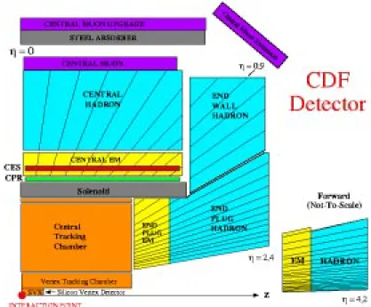
Figure 1.11: The CDF I experimental setup. Central calorimetry is the same as for CDF II.
1.4 The CDF I Detector
25
System range Resolution Thickness CEM j j <1:1 13;7%= p ET 2% 18 X 0 PEM 1:1< j j <2:4 22%= p ET 2% 18-21 X 0 FEM 2:2< j j <4:2 26%= p ET 2% 25 X 0 CHA j j <0:9 50%= p ET 3% 4,5 0 WHA 0:7< j j <1:3 75%= p ET 4% 4,5 0 PHA 1:3< j j <2:4 106%= p ET 6% 5,7 0 FHA 2:4< j j <4:2 137%= p ET 3% 7,7 0
Table 1.2: Angular coverage, resolution and thickness of the CDF I calorimeters.
ET is in GeV.
Central Calorimeter
As already mentioned, this part of the CDF detector was not subject to any substantial change in the CDF II upgrade program.
The Central Calorimeter is azimuthally arranged in 48 physically sepa-rated 15owide modules (wedges) each segmented ininto ten towers [12, 13].
Neighboring towers belonging to dierent wedges are physically separated by not instrumented cracks (\-cracks"), whereas tower separation inside the same wedge is obtained collecting the light from dierent cells into dier-ent PMTs. The boundary between the two halves of the cdier-entral calorimeter and between the wedges and endwall modules constitutes another not instru-mented region (\-cracks").
The Central Electromagnetic Calorimeter (
CEM
) is overlapped by a hadronic section split into two parts, Central Hadronic (CHA
) and Wall Hadronic (WHA
). In each tower both electromagnetic and hadronic sec-tions are read by two PMTs from the opposite faces.Proportional chambers are located between the solenoid and the CEM forming the Central Preradiator Detector (
CPR
) which provides r- infor-mation on electromagnetic showers initiating in the material of the solenoid coil.Located six radiation lengths deep in the CEM calorimeters (approxi-mately at shower maximum) is the Central Electromagnetic Strip Detector (
CES
) [14]. These gas multiwire proportional chambers are divided in each wedge into two halves in z providing pulse height readout in two orthogonal directions: the anode wire channels give the shower pulse height distribu-tion as a funcdistribu-tion of the azimuthal coordinate with the only readout for ve towers, while the cathode strips provide the shower prole along the z1.4 The CDF I Detector
26
a resolution of about 2 cm along both directions.
In front of each -crack dead region is a 12 X0 tungsten bar with a gas
proportional chamber behind it called Central Crack Chamber (
CCR
) [15]. Each of the 48 crack modules has 10 read-out pads in corresponding to the 10 CEM towers. This device allows to detect and measure the energy of electrons and photons falling in such not instrumented zone.1.4.3 Trigger
The CDF I Trigger System was a three level system [6].
Level 1 used fast outputs coming from the muon chambers for muon triggers and from the calorimeters for electrons/photons and jets triggers. Both electromagnetic and hadronic calorimeter towers were summed into trigger towers in a window = 0.215o. The trigger signals from
the detector were sent to the trigger electronics and separately stored until a level 1 decision was made. No deadtime was introduced at this level as a reset signal was sent in time for the next beam crossing if a level 1 accept was not satised at a given crossing. Level 1 calorimeter triggers required the sum of ET for all calorimeter towers (individually above a given threshold,
typically set to 1 GeV) to be greater than a xed threshold (3040 GeV).
At a typical luminosity of 510
30 cm,2s,1 the rate of level 1 triggers was
about 1 kHz.
The level 2 trigger started on a level 1 accept. A hardware clustering processor searched for energetic clusters only considering towers above a programmable threshold. Electromagnetic and hadronic energies were sepa-rately summed up for all towers identied as belonging to the same cluster and the ET, and mean values of the clusters were formed and sorted
in a list. CTC tracks, provided by a fast (10 s) hardware tracking proces-sor (
CFT
), were matched to the electromagnetic clusters and muon system segments to make candidate electrons and muons. The nal trigger was a se-lection on muons, electrons, photons, jets and6~ET. The level 2 trigger outputrate was about 12 Hz.
The third triggering level was constituted by commercial processors read-ing the events selected by the level 2 trigger and submittread-ing them to the same software reconstruction algorithms used in the \o-line" analysis. Most of the execution time was used for the three-dimensional track reconstruction in the CTC. The events accepted by this lter algorithm were nally stored on magnetic tape, with about 5 Hz output rate, for o-line processing.
Chapter 2
Jets at CDF
Jets are among the most interesting \objects" produced by a high energy collider, as they characterize the experimental signature of many known physical events as well as of new physics. Jet physics and phenomenology are described in detail in Appendix A. This chapter describes how jets are reconstructed and corrected in CDF to reproduce well the energy and direction of the partons originating them. The importance of improving the jet energy resolution and its impact on some of the Run II main physics goals is also shown.
2.1 Jet Reconstruction
In a collider experiment a jet appears typically as an energy deposit shared among several calorimeter towers. A reconstruction algorithm is then needed to recognize and reconstruct a jet starting from the energy information on each calorimeter tower.
Fig. 2.1 give us an idea of the jet \development" in the CDF detector. It is the event display of a typical di-jet event where two jets, balancing each other in the transverse plane, are produced.
The CDF jet reconstruction process can be divided into two parts: rst a list of towers is assigned to each jet by a clustering algorithm (the cone algorithm), then the energetic and geometrical information of each tower is combined to reconstruct the jet energy and direction (jet four-momentum). In this section both of them will be described as they were performed in Run I. The cone algorithm implementation for Run II will be almost the same with some dierence due to the changed geometry of the plug calorimeter towers. However complementary algorithms are at present under study [16].
2.1 Jet Reconstruction
28
Run 57920 Event 1780 jet20_t.pad 5APR94 11:32:14 11-Nov-00 Pt Phi Eta z_1= 20.7, 31 trk 15.7 311 -0.48 13.7 123 -0.66 -11.9 311 -0.47 6.3 116 -0.50 -5.0 316 -0.44 -4.0 123 -0.65 2.7 120 -0.52 1.9 313 -0.21 -1.2 120 -0.91 1.1 320 -0.91 -0.9 121 -0.30 0.9 125 -0.58 0.8 297 -0.20 -0.7 331 1.10 -0.6 129 -0.78 -0.6 66 -0.96 0.5 85 -1.09 -0.5 153 0.15 0.5 347 -1.29 -0.4 139 0.46 -0.4 132 -0.68 0.4 302 1.34 0.4 19 -0.36 -0.4 132 -1.39 -0.4 9 -0.32 -0.4 348 0.19 0.3 144 -1.15 -0.3 359 -1.02 0.3 230 -1.00 0.2 25 -0.67 0.2 13 0.71 4 unattchd trks -0.4 298 0.32 3 more trks...
hit & to display PHI:
ETA: 311. -0.48 Emax = 32.7 GeV Et(METS)= 6.6 GeV / Phi = 147.5 Deg Sum Et = 100.3 GeV
Run 57920 Event 1780 jet20_t.pad 5APR94 11:32:14 11-Nov-00
PHI: ETA:
311. -0.48 14.6
DAIS E transverse Eta-Phi LEGO Plot
Max tower E= 14.6 Min tower E= 0.10 N clusters=
METS: Etotal = 425.8 GeV, Et(scalar)= 100.3 Ge Et(miss)= 6.6 at Phi= 147.5 Deg.
Cluster Et_min 0.0 GeV Clusters:ETHAT CLUSTERING $CLP: Cone-size= 0.7, Min Tower Et= 0.1 EM HA Nr Et Phi Eta DEta #Tow EM/Et Trks Mass 3 36.0 309.7 -0.45 -0.36 0 0.535 6 6.4 2 31.7 122.2 -0.61 -0.51 0 0.747 8 6.4 R= 0.7 PHI: ETA: 311. -0.48
Figure 2.1: A typical CDF event where two jets are produced balancing each other in the transverse plane. The CTC-plot (upper) allows to see the charged particles (mainly ) associated to the jet while the lego-plot (lower) shows the jet energy
sharing among the calorimeter towers. The electromagnetic deposit (magenta) is mainly due to 0
! while the hadronic one (blue) is due to both charged and
neutral hadrons. Only towers with energy above the clustering threshold (0.1 GeV) are shown. Also shown is the reconstruction cone radius set to 0.7.
2.1 Jet Reconstruction
29
2.1.1 CDF Jet Clustering Algorithm
The CDF jet clustering algorithm uses a cone of a xed radius to dene a jet, the CDF calorimeter towers being its basic units. Energetic towers are assigned to jet clusters by an o-line routine (JETCLU) [17, 18] implementing the jet-nding algorithm in three steps:
Preclustering
: a list of \seed towers" above a xed ET threshold(set to 1.0 GeV) is created and sorted in order of decreasing ET. In
the plug and forward calorimeters, towers are grouped together in sets of three in to have a = 15o segmentation corresponding to the
central one. Seed towers are grouped into preclusters consisting of an unbroken chain of continuous towers with decreasing energy. If a tower is outside a 77 window around the largest ET seed, it is used to form
another precluster. The precluster list is the starting point for the next step.
Cone algorithm
: using the true tower segmentation, theET weightedcentroid of each precluster is found and a cone in- space of radius R (typically R = 0.4, 0.7 and 1.0) is formed around it 1. A loop is then
performed over all towers with ET above 0.1 GeV, including them in
a cluster if their centroid is inside the cone around it. A new cluster centroid is then recalculated from the new set of towers belonging to it and a new cone is drawn around this position. The loop over towers is repeated using the new centroid. This process is iterated until the tower list for each cluster remains unchanged in two consecutive passes.
Merging and/or solving overlaps
: the cone algorithm is such thatin multijet events two clusters can overlap with some towers being assigned to more than one cluster. In this step clusters are merged into one or left alone so to have each tower uniquely assigned to a cluster. When one cluster is completely contained in another, the smaller of the two is dropped. In the overlapping situation, an overlap fraction is dened as the ET sum of the common towers divided by the ET of
the smaller cluster. When this fraction is above a cuto (usually 0.75) the two clusters are combined into one, otherwise they are kept intact assigning each tower in the overlap region to the closest cluster in -
space. Finally, after the cluster separation or merging, the new centroid of each cluster is recalculated using the new tower list.
1R is usually referred as \cone radius" and is chosen to best t the jet topology of each
2.2 Jet Energy Corrections
30
2.1.2 Jet Energy and Momentum Reconstruction
From the list of towers associated with the cluster, JETCLU then calculates the jet four-momentum components according the following denitions:
EJ = N X i=1 Ei (2.1) Px;J = N X i=1 Eisinicosi (2.2) Py;J = N X i=1 Eisinisini (2.3) Pz;J = N X i=1 Eicosi (2.4)
where i is the tower index and N the number of towers in the cluster. The angles i are evaluated according to the CDF coordinate system (see
Chap-ter 1) while the angles i are calculated respect to the event vertex along the
beam axis.
Note that, according to these denitions, jets are not massless.
Using the above quantities, the jet transverse energy and momentumET;J
and PT;J are dened as:
PJ = q P2 x;J+P2 y;J +P2 z;J (2.5) PT;J = q P2 x;J+P2 y;J (2.6) ET;J =EJPPT;JJ (2.7)
2.2 Jet Energy Corrections
As will be shown in next chapter, the jet energy is aected by mismeasure-ment due both to physics and to detector eects. So proper corrections need to be applied in order to reconstruct, from the measured jet PT, the true
momentum of the parton generating it [18]. The pure reconstructed jet ET
2.2 Jet Energy Corrections
31
2.2.1 JTC96 Jet Corrections
In this section we describe the standard CDF jet corrections used in Run I and which we will consider as a reference in the following of the present thesis. Analogous corrections will be developed for Run II using new data and new Monte Carlo samples accounting for the dierent run and detector conditions.
These corrections are usually referenced as \
JTC96 Jet Corrections
" (being implemented by the o-line routine JTC96 [19, 20]) and are performed in four separate steps:
Relative
corrections: accounting for the eects of gaps and edgesin-side the calorimeters (\-cracks") and for non-uniform response of dif-ferent calorimeters.
Absolute
corrections: correcting for non-linear response of thecalorime-ters to low momentum particles and for eects due to not detected fragmentation products. The true parton PT is estimated from the
observed raw jet PT.
Underlying Event (UE)
corrections: the contribution to the jet PTcoming from energy not associated with the hard scattering process is estimated and subtracted.
Out-Of-Cone (OOC)
corrections: a fragmentation model is used toestimate the amount of jet energy carried by particles going outside the clustering cone. Such quantity is then used to correct the jet PT.
A brief description of the method used to extract each correction will be now given.
Relative Corrections
-cracks eects and possible dierences in the detector response among the central, plug and forward calorimeters are accounted for by these corrections providing an uniform jet response as function of .
The corrections are parametrized as a function of the jet and raw PT
and are derived by equating inPT all jets to an equivalent central jet [19, 20].
The central region (usually in the 0:2 jj 0:7 range so to be far from
cracks) is considered because here the calorimeter response is at and non-linearities are well understood from extensive test-beam measurements and checked during data acquisition using tracking informations.
To perform such corrections di-jet events, with at least one central jet, are selected and a relative response function is extracted requiring the PT
2.2 Jet Energy Corrections
32
back-to-back balancing of the central jet (usually referred as \trigger jet") with the other one (usually referred as \probe jet") falling in each calorimetric region. A dependence of such function on the probe jet is considered.
Di-jet events are selected from the \jet triggers" data samples according the following cuts:
At least one (\trigger") jet at 0:2jj0:7. One additional (\probe") jet with PT >15 GeV/c. No other jets with PT >15 GeV/c.
z coordinate of the event vertex jzj60 cm. One vertex in the event
2.
J
1,J2 >2.7 radians.
Bias eects from the on-line trigger cut, are avoided requiring PT(Raw) for
the two leading jets to exceed twice the single jet trigger threshold value. In a perfect detector, from momentum conservation in the transverse plane, the missing ET (6~ET) variable (dened in CDF as the vectorial sum
over all energetic towers above a xed threshold - usually 0.1 GeV - with jj < 3.6) is expected to have a very low value being randomly directed in each direction. The occurrence of a high value of such variable (usually above a given trigger threshold) is used to indirectly indicate the presence of an undetected neutrino.
A neutrino is not present in a typical di-jet event, so the6~ET is attributed
to jet mismeasurements and is expected to be correlated to their directions (see also section 4.2.3).
We call 6~ET projection fraction (MPF) the ratio between the 6~ET vector
projection along the ~PTProbe vector direction (PbProbe
T ) and the mean value of
PTProbe and PTrigger T : MPF = 2(6~ET b PTProbe) PTProbe+PTrigger T In the 6E T PTProbe hypothesis, 6~ET b PTProbe 'P Trigger T ,PTProbe. So we obtain: MPF = 2(PTTrigger,PTProbe) PTrigger T +PTProbe
2For Run Ib this cut was loosened to two in order to improve the statistics, as a large
2.2 Jet Energy Corrections
33
Finally, dening the relative jet scale correction factor as
= PTTrigger
PTProbe
we get
= 2 +2 MPF
,MPF
which results to be a function of PT and .
The relative corrections are derived by tting the distribution with a continuous curve as a function of the probe jet in dierent PT(Raw)
ranges [20].
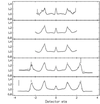
Figure 2.2 reports the Run Ib relative corrections obtained with this method.
Figure 2.2: Run Ib relative corrections for a cone radius R = 0.4 [20]. Each
PT bin (mean values from top to bottom: 363, 241, 172, 125 and 64 GeV/c)
corresponds to each jet trigger sample: JET20, JET50, JET70 and JET100. The eect of \-cracks" is in particular evident.
Absolute Corrections
These corrections are introduced to get the best energy estimate of the orig-inal parton generating the jet. The parton energy is usually underestimated mainly because of nuclear absorption, particle leakage and nonlinear calori-meter response.
2.2 Jet Energy Corrections
34
Monte Carlo simulations are used to obtain these corrections according the following denitions:
A given parton is associated to a jet if their directions are close in the - space below a xed distance (usually R < 0.4).
The jetPT is evaluated summing thePT of all particles falling into the
clustering cone.
A PT dependent correction factor is dened as the ratio between the
parton PT and the jet raw PT:
(PT) =< PPJetTParton T (Raw) >
Because of the nonlinearity in calorimeter response, the observed jet en-ergy is a function not only of the incident parton enen-ergy but also of the momentum spectrum of the particles produced in the jet fragmentation. Par-ticular attention was so made in order to properly reproduce in the simulation the observed jet fragmentation. The parameters of the Monte Carlo event generator accounting for parton fragmentation (SETPRT), implemented in the QFL simulation package of CDF, were tuned in order to reproduce the longitudinal and transverse (charged) fragmentation properties observed us-ing the CTC [18].
Underlying Event Corrections
The underlying event corrections (
UE
) take into account all the contributions to the jet energy not coming from the original parton. Hadron collisions are in fact characterized by an \ambient energy" (usually referred as underlying event) which is produced by soft interactions of spectator partons (the \beam-beam remnants") and by initial state gluon radiation (ISR) eects [18, 21] (see g. 2.3).Both data and Monte Carlo samples are used to study the UE eects. The (ambient) energy density, to be used in the UE corrections, is estimated from \minimum bias" events3 considering the
P
ET over the calorimeter towers
for jj 1.0, normalized to the overall coverage. The absolute correction
factor is applied to the tower energy to get the correction at parton level. It is clear that for a bigger jet reconstruction cone, a bigger UE incidence is observed so these corrections need to be derived for dierent jet cones.
3Minimum-bias events are selected by a trigger just demanding the occurrence of a
2.2 Jet Energy Corrections
35
Figure 2.3: Illustration of two typical pp collisions with a \hard" 2-to-2 parton
scattering originating a di-jet event. Top: only a primary interaction is present. The nal state contains particles coming from the two outgoing partons (\true"
jet particles), including the nal state radiation (FSR), and particles coming from the UE. The UE consists of the beam-beam remnants plus ISR. Bottom: a multiple parton interaction has occurred. In addition to the \hard" 2-to-2 parton scattering also a \semi-hard" one is present contributing particles to the UE.
Moreover, as the UE eects are also due to particles coming from other in-teractions in the same bunch crossing (multiple vertices), the UE corrections are also parametrized in function of the the number of vertices in the event (Nv) found by the SVX. Table 2.1 shows the dierent parametrization of
these corrections for the three jet reconstruction cones, with a dependence on Nv. No PTParton dependence is observed for these corrections.
2.2 Jet Energy Corrections
36
Clustering Cone 0.4 0.7 1.0
UE for MC 0.370 1.133 2.312
UE for data (a) 0.297N 0.910N 1.858N
UE for data (b) 0.65 1.98 4.05
OOC for data and MC 1.95+0.156PT 1.29+0.052PT 0.54+0.022PT
Table 2.1: UE and OOC corrections used in JTC96. N = Nv - 1, Nv being
the number of vertices found in the same pp bunch crossing. Line (a) must be
subtracted before absolute corrections (to have a better jet raw PT estimate), line
(b) after them. The OOC corrections are added as last step. All values are given in GeV.
Out-of-Cone Corrections
The out-of-cone (
OOC
) corrections recover the jet energy falling out of the clustering cone because of fragmentation eects and gluon radiation (see g. 2.3 top).The study of cone losses is performed with the same Monte Carlo sample used to obtain the absolute corrections. A dependence on the reconstruction cone size is obviously expected. The correction is dened as:
POOC(PT;R) = PTParton
,P
Jet T
where PTParton is given by the sum of the PT of all particles coming from the
parton while PTJet is given by the sum of the PT of all particles coming from
the parton and falling inside the reconstruction cone. POOC can be linearly
parametrized as a PT function, as shown in table 2.1.
2.2.2 Uncertainties in Energy Scale
The absolute jet energy scale is subject to a systematic error mainly due to the uncertainties in the single-particle response of the calorimeters and in the jet fragmentation function. Dedicated studies have shown an uncertainty ranging from 10% for low ET jets (ET 25 GeV) to 4% for very
energetic central jets (0:1 jj 0:7) [18]. Usually a 5% uncertainty is
quoted in most of analyses where high-ET central jets are present.
2.2.3 Specic Corrections
The standard JTC96 jet corrections are not suitable in reconstructing the right energy for jets generated by b-quark fragmentation (b-jets). The
ana-2.3 Jets in Physics Events
37
lysis of HERWIG tt Monte Carlo samples has in fact shown signicant dis-agreements between reconstructed and primary parton energies [22]. The origin of this disagreement can be traced on the fact that b-jets are charac-terized by a secondary decay vertex inside them due to B hadron decay. So a relevant part of the jet energy can be carried away by additional particles going outside the clustering cone or by a not detected neutrino or a muon (not interacting in the calorimeters) which are generated in the semileptonic B hadron decay.
On the other hand the b-quarks jets occurrence is typical of top-quark production so, for the top mass analysis, an additional set of jet corrections (usually referred a \AA Corrections") has been developed to be applied after the JTC96 ones so to bring the jet energy to agree with the HERWIG parton energy [22] 4.
The AA corrections are applied using a parametrization which depends on the B hadron decay mode (i.e. distinguishing if semileptonic or not and, in the former occurrence, if an electron or a muon is present). The parameters are obtained with a tting method using the HERWIG Monte Carlo.
2.3 Jets in Physics Events
As already mentioned, many interesting physics signatures in an experiment like CDF have quarks or gluons in the nal state which, because of the frag-mentation process, experimentally appear as hadronic jets. The importance of improving the jet energy resolution is then evident. In the following, while briey describing the CDF II physics search program, we will give two im-portant examples where an improved jet energy resolution will play a leading role: top quark mass measurement and light Higgs search.
2.3.1 The CDF II Physics Program
Several elds of interest in particle physics will be investigated in Run II data analysis [5]. The CDF II physics program can be summarized into ve main goals:
Top quark properties studies.
Higgs boson and new phenomena beyond the SM direct search.
4These corrections are indeed fundamental in every analysis where b-jet characterize
the nal state. An example is given by the Higgs boson search in the associate production channel WH!Wbb.
2.3 Jets in Physics Events
38
Precision electroweak physics measurements. B meson physics.
Test of perturbative QCD at NLO and large Q 2.
The two measurements more sensitive to the jet energy resolution will be now detailed.
Top Quark Mass
The most important physics result obtained by the CDF collaboration in Run I was the discovery of the top quark and the rst direct measurement of its mass and cross section [6, 23] (see g. 2.4).
Combined with the W mass,mtopgives information about the mass of the
Higgs boson, the missing particle foreseen by the Standard Model. Fig. 2.5 shows the predicted limits on the Higgs mass given by the present resolutions on top and W masses. It is so evident that the top quark mass will be one of the most important electroweak measurements performed at the Tevatron in Run II.
Currently, the statistical and systematic uncertainties on CDF top mass measurement are both about 5 GeV. The statistical uncertainty should scale as 1=p
N. The CDF collaboration is condent to reduce it to 1 GeV/c 2
in the optimized lepton +4-jet sample with at least one b-tagged jet [5].
In Run II, systematics will dominate the uncertainty on mtop. With the
new integrated tracking, the acceptance for double-tagged lepton + 4-jet
events can increase by about a factor of 2.5. In these events, the probability of misassociation among jet and parton is lower. By reducing this kind of systematic uncertainty, the top mass resolution will improve by 20%.
Moreover the systematics due to the b-tagging bias may be better understood for this class of events.
Almost all the remaining systematics in the measurement of mtop are
coupled to the reliability of the Monte Carlo models to get the spectrum of t masses in signal and background. Assuming an accurate theory model, most of the uncertainty is related to detector resolution eects. Instrumental contribution include calorimeter nonlinearity, losses in cracks, de