Department of Economics
Working Paper No. 244
Structural breaks in Taylor rule based
exchange rate models - Evidence from
threshold time varying parameter
models
Florian Huber
Structural breaks in Taylor rule based exchange rate models - Evidence from threshold time varying parameter models
Florian Huber∗
Vienna University of Economics and Business
Abstract
In this note we develop a Taylor rule based empirical exchange rate model for eleven major currencies that endogenously determines the number of structural breaks in the coefficients. Using a constant parameter specification and a standard time-varying pa-rameter model as competitors reveals that our flexible modeling framework yields more precise density forecasts for all major currencies under scrutiny over the last 24 years.
Keywords: Stochastic volatility, mixture innovation models, time-varying parameters
JEL Codes: E52, F31, F42.
1 Introduction
Since the seminal contribution ofMeese and Rogoff(1983) showed that empirical exchange rate models fail to outperform simple random walk specifications, a plethora of literature aimed to improve the predictive capabilities of empirical exchange rate models (see the dis-cussion inRossi,2013). Recently,Molodtsova and Papell(2009) provide some evidence that Taylor rule based exchange rate models outperform other structural models in terms of out-of-sample predictive performance. However, this branch of the literature typically assumes constant coefficients in the exchange rate equation, effectively imposing strong restrictions on the underlying causal relationships (some exceptions areCanova,1993;Abbate and Mar-cellino,2014;Byrne et al.,2016;Huber,2016). Evidence on time-varying Taylor rules (Byrne et al.,2016) suggests that it pays off to allow for time-variation in the underlying structural parameters.
In this note, we apply a recent econometric methodology put forward in Huber et al.
(2016) to a set of eleven exchange rate pairs and assess whether using a threshold time-varying parameter model (TTVP) improves the out-of-sample predictive performance. Our model is benchmarked against a standard time-varying parameter model with stochastic volatility (TVP-SV) and a constant parameter model.
∗
Corresponding author: Florian Huber, Vienna University of Economics and Business, Phone: +43-1-313 36-4534. E-mail:[email protected].
2 A flexible empirical framework to model exchange rates
We apply our modeling framework to the exchange rate of eleven economies relative to the US dollar, namely the United Kingdom, Japan, Canada, Australia, Germany, Italy, Netherlands, France, Denmark, Sweden and Switzerland. FollowingMolodtsova et al.(2008);Molodtsova and Papell(2009) and Molodtsova et al.(2011), we assume that both countries’ monetary policy reaction function is described by a (symmetric) Taylor rule, leading to the following exchange rate equation between the home and the foreign countryf
∆st=β0−βπU Sπt+βπfπ˜t+γuU Sut−γufu˜t−κU Si it−1+κfi˜it−1+εt. (2.1)
Here we let∆st (t = 1983 : M01, . . . , T = 2014 : M12)denote the monthly change in the
nominal exchange rate measured as the price of countryfth currency in terms of the home currency and ∼ marks foreign variables. Thus ∆st > 0 implies an depreciation of the US
dollar. Furthermore πt denotes month-on-month CPI inflation and ut denotes the civilian
unemployment rate to measure the output gap1. Moreover we leti
tdenote the three-month
money market rate. For the Euro Area countries, we link the exchange rate series with the EUR/USD exchange rate after the Euro has been introduced. Finally,εt∼ N(0, σj2)is a white
noise process with constant varianceσj2.
The corresponding regression coefficients β = (β0,−βπU S, β f π, γU Su ,−γ f u,−κU Si , κ f i) and the error variancesσ2j are typically assumed to be constant over time. In this note we as-sess whether it improves predictive abilities if we allow for movements in the parameters of
Eq. (2.1). More specifically, we estimate the following model,
∆st=Xtβt+εt, εt∼ N(0, eht), (2.2)
with Xt being a stacked vector of data. To closely mimic the information set available to
the forecaster at timet we assume that macroeconomic variables are available only with a one-period lag while short-term interest rates are available in real-time.
Each element ofβt,βkt(k= 1, . . . ,7), evolves as
βkt=βkt−1+dktϑkηkt, (2.3)
where ηkt ∼ N(0,1) and ϑ2k denotes the error variance of the latent states. Moreover, dkt
denotes the indicator function that equals unity if the absolute change inβkt,|∆βkt|is large
enough, i.e. exceeds a certain thresholdck. This implies that if |∆βkt| < ck, dkt = 0 and
βkt =βkt−1, meaning that thejth coefficient is kept constant fromt−1tot. Finally, we let
htdenote the log-volatility that evolves according to a first-order autoregressive process (see
Kastner and Fr¨uhwirth-Schnatter,2014).
This modeling approach has been introduced inHuber et al.(2016) to search for appropri-ate model specifications over time. As compared to a standard time-varying parameter model that setsdkt= 1for allk, t, our model allows to discriminate between periods where
param-eters have been moving significantly over time or periods where paramparam-eters remained rela-tively constant. While a standard TVP model imposes the restriction that parameters evolve 1We have experimented with (detrended) industrial production to measure real activity. The results appear
smoothly over time, our threshold TVP model is capable of accommodating large swings in the respective parameters. Moreover, our model is also able to detect cases where elements ofβtdisplay only a relatively low number of structural breaks. In addition, through Bayesian
shrinkage priors, our model also investigates whether certain parameters inEq. (2.1)should be set equal to zero. This captures the notion that some central banks do not react to move-ments in the output gap (i.e.βuf = 0) or perform interest rate smoothing (i.e.β
f i = 0).2
Our model thus endogenously detects whether we need a model with a low, moderate or a large number of structural breaks. Especially for Taylor rule based models, the question whether the monetary policy reaction function of a given central bank remained constant over time is questionable. For instance, it could be the case that the central bank does not change its stance towards inflationary developments over time but aggressively targets the output gap during crisis periods. The proposed model is capable of detecting such regime shifts in a data-based fashion.
3 Forecasting results
In this section we perform a forecasting horse race using three models. The first one is a constant parameter model given byEq. (2.1). The second specification is the threshold TVP (TTVP) model and the final model adopted is a standard TVP model (i.e.dkt= 1for allk, t).
We estimate all models using Bayesian methods. The prior specification and the corre-sponding Markov chain Monte Carlo algorithm adopted for all models is described in more detail inHuber et al.(2016). For the constant parameter model we use relatively uninforma-tive priors on the regression coefficients and an inverted Gamma prior onσj2 with scale and shape parameter equal to0.01.
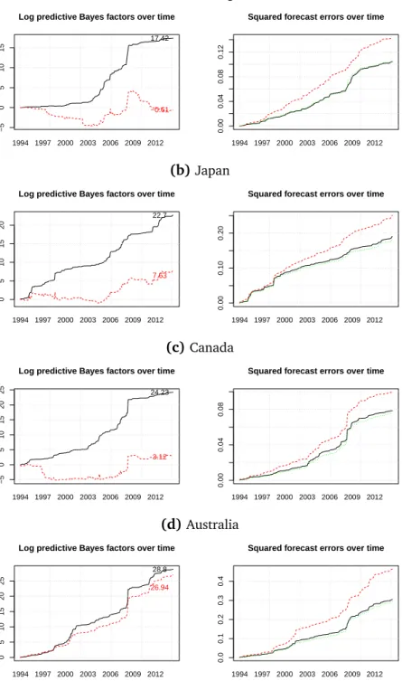
Our forecasting design relies on rolling window estimation. We use the period ranging from 1983:M01 to 1994:M01 (132 observations) as an initial estimation sample and the re-maining 352 (24 years) observations as an hold-out sample. We compute the one-step-ahead predictive density for each point in our hold-out sample and consequently move the estima-tion sample by a single observaestima-tion forward while dropping the first observaestima-tion. This pro-vides us with a sequence of 352 predictive densities, a comparatively large hold-out sample. Because previous studies devoted most attention to point forecasts, we focus mainly on the log predictive score, a typical Bayesian criterion to evaluate model predictions (seeGeweke and Amisano, 2010, for a discussion on the log predictive likelihood). Moreover, we also briefly assess the out-of-sample fit by investigating the evolution of the cumulative squared forecast errors.
Figure1 depicts the evolution of the log predictive score (LPS, left panel) and the cumu-lative squared forecast errors (right panel) over the hold-out sample for all countries under consideration.
[Fig. 1 about here.]
The figure reveals that for all eleven currencies, the TTVP model outperforms both, a con-stant parameter model (indicated by positive values of the relative LPS) and the TVP model.
The results for the TVP model suggest that for the United Kingdom and Canada, the simple linear regression model outperforms the more flexible time-varying parameter model. This result can be traced back to the fact that we rely on a rolling window forecasting design that keeps the number of observation used in the estimation fixed. A heavily parameterized model like the TVP specification features a high dimensional state vector, implying that the number of parameters to be inferred is large relative to the number of available observations, leading to overfitting issues.3 Visual inspection of the corresponding predictive densities (not shown) corroborates these findings. Taken at face value our results indicate that the amount of shrinkage on the time-variation andthe initial state supplied by the TTVP framework al-leviates overfitting problems effectively, providing a parsimonious model that is useful for a large battery of exchange rates.
The steep increase in predictive accuracy, as measured by the LPS, during and after the global financial crisis may be attributed to two distinct sources. The first source is that most central banks in developed economies aggressively lowered interest rates, reaching the zero lower bound (ZLB) within one year after the Lehman event. While a constant parameter specification is not able to fully capture these developments, flexible time-varying parameter models can account for such changes in the policy rule. The second reason for the pronounced improvements in LPS is that the linear model assumes that the volatility of the shocks remains constant, implying that the variance of the corresponding predictive density is either too large or too low. Thus, during tranquil periods, the predictive variance is elevated whereas during crisis episodes a constant parameter specification effectively underestimates the predictive variance, rendering it almost impossible to capture economic outliers. Comparing the perfor-mance differences between both time-varying parameter models suggests that our threshold specification allows for more abrupt changes in the underlying Taylor rule coefficients. Such pronounced structural breaks match actual movements of central banks much better than the gradual adjustments implied by a standard random walk state equation that is used in the TVP model.
Zooming into specific results for individual countries reveals that especially during id-iosyncratic events like the exchange rate market intervention conducted by the Swiss national bank (seeFig. 1 (k)) in 2011 to ease the appreciation of the Franc, our TTVP model yields marked accuracy gains. Interestingly, for the case of the Swiss Franc we see that the TTVP sharply improves upon a linear specification while the TVP specification loses some momen-tum against the constant parameter model (as can be seen in the decline in relative LPS in the second half of 2011).
For Germany, Italy, Netherlands and France we observe that the TVP model produced forecasts that have been slightly superior relative to the TTVP model until the beginning of the 2000s. After the Euro has been introduced, however, allowing for flexible error variance specification in the state equation generally pays off. Moreover, for most Euro area coun-tries we observe that during the recent crisis of the Euro area, both time-varying parameter models sharply outperform the linear benchmark model, effectively controlling for the fact that a simple Taylor rule provides a rather poor approximation of actual monetary policy im-3In fact, using a recursive forecasting design shows that the performance differences between the TTVP and
plemented by the ECB during that time frame. Technically speaking, we conjecture that the reason behind these marked gains is that the TTVP framework allows for much larger swings in the underlying parameters since the marginal posterior distributions of the state innovation variances have heavier tails as compared to the ones of a standard TVP model. This feature of our model implies much faster adjustment dynamics of the underlying structural coefficients which directly translates into better calibrated predictive densities.
Before we proceed to the discussion of the point forecasts, a brief word on statistical significance is in order. We assess the significance of differences in LPS by means of the test stipulated in Amisano and Giacomini(2007). For all currencies, the differences in LPS between the TTVP and the constant specification appear to be significant at conventional levels. For the standard TVP specification we find that the differences in LPS terms for the British pound and the Swedish krona are not significant at the five percent level.
Turning to the point forecasts as indicated by the cumulative squared forecast errors re-veals that for all currency pairs, the TTVP model yields more precise point predictions as compared to the TVP model. Thus, the gains in predictive accuracy as measured by the LPS could stem from both, more precise point and variance predictions. Interestingly, the linear model provides point forecasts that appear to be marginally more precise as the predictions obtained from the TTVP specification for most currencies. It is noteworthy that this implies that the pronounced improvements in terms of density predictions stem from other features of the predictive density (i.e. the predictive variance). Since the bulk of accuracy improvement appears to originate from better variance predictions we conclude that a good exchange rate model should entail both, some form of structural breaks in the regression coefficientsand some form of heteroscedasticity in the errors ofEq. (2.1).
4 Conclusive remarks
In this note, we apply a flexible econometric framework to a set of eleven exchange rates. Our empirical model is based on a Taylor rule specification that allows for time-variation in the Taylor rule parameters and stochastic volatility in the errors. This model is then used in a forecasting exercise where we investigate how the log predictive score and the squared fore-cast errors evolve over time. Our finding suggests that especially during periods of financial stress it pays off to have a more flexible econometric specification. We would like to stress that our findings are currently confined to Taylor rule based exchange rate models. Further analysis that devotes attention to other structural exchange rate models as in Byrne et al.
(2016) could improve the generality of our findings. References
Abbate A and Marcellino M (2014) Modelling and forecasting exchange rates with time-varying parameter models*. Journal of Economic Literature
Amisano G and Giacomini R (2007) Comparing density forecasts via weighted likelihood ratio tests. Journal of Business & Economic Statistics25(2), 177–190
Byrne JP, Korobilis D and Ribeiro PJ (2016) Exchange rate predictability in a changing world. Journal of International Money and Finance62, 1–24
Canova F (1993) Modelling and forecasting exchange rates with a Bayesian time-varying coefficient model. Journal of Economic Dynamics and Control17(1-2), 233–261
Geweke J and Amisano G (2010) Comparing and evaluating Bayesian predictive distributions of asset returns. International Journal of Forecasting26(2), 216–230
Huber F (2016) Forecasting exchange rates using multivariate threshold models. The BE Journal of Macroeconomics16(1), 193–210
Huber F, Kastner G and Feldkircher M (2016) The threshold time-varying parameter (TTVP) model. arXiv preprint arXiv:1607.04532
Kastner G and Fr¨uhwirth-Schnatter S (2014) Ancillarity-sufficiency interweaving strategy (ASIS) for boosting MCMC estimation of stochastic volatility models. Computational Statistics & Data Analysis76, 408–423
Meese RA and Rogoff K (1983) Empirical exchange rate models of the seventies: Do they fit out of sample? Journal of International Economics14(1), 3–24
Molodtsova T, Nikolsko-Rzhevskyy A and Papell DH (2008) Taylor rules with real-time data: A tale of two countries and one exchange rate. Journal of Monetary Economics55, S63–S79 Molodtsova T, Nikolsko-Rzhevskyy A and Papell DH (2011) Taylor rules and the euro.Journal
of Money, Credit and Banking43(2-3), 535–552
Molodtsova T and Papell DH (2009) Out-of-sample exchange rate predictability with Taylor rule fundamentals. Journal of International Economics77(2), 167–180
Fig. 1:Evolution of the cumulative log predictive score and squared forecast errors over time
(a)United Kingdom
−5
0
5
10
15
Log predictive Bayes factors over time
1994 1997 2000 2003 2006 2009 2012 17.42 −0.61 0.00 0.04 0.08 0.12
Squared forecast errors over time
1994 1997 2000 2003 2006 2009 2012 (b)Japan 0 5 10 15 20
Log predictive Bayes factors over time
1994 1997 2000 2003 2006 2009 2012 22.7 7.63 0.00 0.10 0.20
Squared forecast errors over time
1994 1997 2000 2003 2006 2009 2012 (c)Canada −5 0 5 10 15 20 25
Log predictive Bayes factors over time
1994 1997 2000 2003 2006 2009 2012 24.23 3.12 0.00 0.04 0.08
Squared forecast errors over time
1994 1997 2000 2003 2006 2009 2012 (d)Australia 0 5 10 15 20 25
Log predictive Bayes factors over time
1994 1997 2000 2003 2006 2009 2012 28.8 26.94 0.0 0.1 0.2 0.3 0.4
Squared forecast errors over time
1994 1997 2000 2003 2006 2009 2012
Notes: The figures show the evolution of the cumulative LPS relative to the constant parameter model (left panel) and the cumulative squared forecast errors (right panel) for the threshold time-varying parameter (in solid black), time-varying parameter (in dashed red) and constant parameter (in dashed green) specifications. The results are based on 15,000 posterior draws.
(e)Germany 0 5 10 15 20
Log predictive Bayes factors over time
1994 1997 2000 2003 2006 2009 2012 20.41 14.64 0.0 0.1 0.2 0.3
Squared forecast errors over time
1994 1997 2000 2003 2006 2009 2012 (f)Italy 0 5 10 15
Log predictive Bayes factors over time
1994 1997 2000 2003 2006 2009 2012 16.91 13.46 0.0 0.1 0.2 0.3
Squared forecast errors over time
1994 1997 2000 2003 2006 2009 2012 (g)Netherlands 0 5 10 15 20
Log predictive Bayes factors over time
1994 1997 2000 2003 2006 2009 2012 21.33 19.65 0.0 0.1 0.2 0.3
Squared forecast errors over time
1994 1997 2000 2003 2006 2009 2012 (h)France 0 5 10 15
Log predictive Bayes factors over time
1994 1997 2000 2003 2006 2009 2012 19.05 17.86 0.0 0.1 0.2 0.3
Squared forecast errors over time
1994 1997 2000 2003 2006 2009 2012
Notes: The figures show the evolution of the cumulative LPS relative to the constant parameter model (left panel) and the cumulative squared forecast errors (right panel) for the threshold time-varying parameter (in solid black), time-varying parameter (in dashed red) and constant parameter (in dashed green) specifications. The results are based on 15,000 posterior draws.
(i)Denmark
0
5
10
15
Log predictive Bayes factors over time
1994 1997 2000 2003 2006 2009 2012 17.11 15.43 0.0 0.1 0.2 0.3
Squared forecast errors over time
1994 1997 2000 2003 2006 2009 2012 (j)Sweden −5 0 5 10 15 20
Log predictive Bayes factors over time
1994 1997 2000 2003 2006 2009 2012 23.05 1.22 0.00 0.05 0.10 0.15 0.20
Squared forecast errors over time
1994 1997 2000 2003 2006 2009 2012 (k)Switzerland 0 5 10 15 20
Log predictive Bayes factors over time
1994 1997 2000 2003 2006 2009 2012 23.84 1.63 0.00 0.10 0.20
Squared forecast errors over time
1994 1997 2000 2003 2006 2009 2012
Notes: The figures show the evolution of the cumulative LPS relative to the constant parameter model (left panel) and the cumulative squared forecast errors (right panel) for the threshold time-varying parameter (in solid black), time-varying parameter (in dashed red) and constant parameter (in dashed green) specifications. The results are based on 15,000 posterior draws.