User s Guide for ContactCenters Simulation Library

(1)

User’s Guide for ContactCenters Simulation Library

Generic Simulator for Blend and Multi-skill Call Centers

Version: March 17, 2014

Eric Buist

This document introduces a generic simulator for blend and multi-skill call centers. The simulator is written using Java, SSJ, and the ContactCenters library. It is configured using XML files and supports call centers with inbound and outbound calls of multiple types, multiple groups of agents, and complex routing policies. This document presents the model implemented by the simulator, the format of the configuration files with some examples, and instructions to run the simulator from the command-line and to extend it internally in Java code. We also provide a reference guide documenting every supported parameter and performance measure. In this document, any reference to a contact corresponds to a call, since the simulator only considers calls as type of contacts.

(2)

Reference documentation

140

7 Overview 140

8 The XML format used by the simulator 141

8.1 Overview of the XML format . . . 141

8.2 Supported data types . . . 142

8.2.1 Simple data types . . . 143

8.2.2 Complex data types . . . 144

8.3 Available arrival processes . . . 145

8.4 Available dialer’s policies . . . 150

8.5 Available router’s policies . . . 154

9 Types of experiments 165 9.1 Finite horizon . . . 165

9.2 Steady-state . . . 166

10 The output of the simulator 169 10.1 The contents of a report . . . 169

10.2 The format of the report . . . 171

10.2.1 Program-readable format . . . 171

10.2.2 Plain text . . . 171

10.2.3 Microsoft Excel . . . 172

10.2.4 Localized format for reports . . . 172

10.3 Available performance measures . . . 173

10.4 Supported row types . . . 194

10.5 Supported column types . . . 196

(6)

List of Tables

1 Parameters for the most commonly used probability distributions . . . 21

2 Parameters in the Web form for CCmath with corresponding parameters in the sim2skill.xmlfile . . . 44

3 XML entities used to escape reserved characters . . . 142

4 Supported symbols for time units . . . 143

5 Most common Java properties affecting reporting . . . 172

(7)

vi

LIST OF FIGURES March 17, 2014

List of Figures

1 The Implemented Model of Call Center . . . 4

2 The simulated horizon . . . 5

3 The path of a call in the call center . . . 6

4 The path of an outbound call in the call center . . . 8

5 The transfer of a call to a secondary agent . . . 11

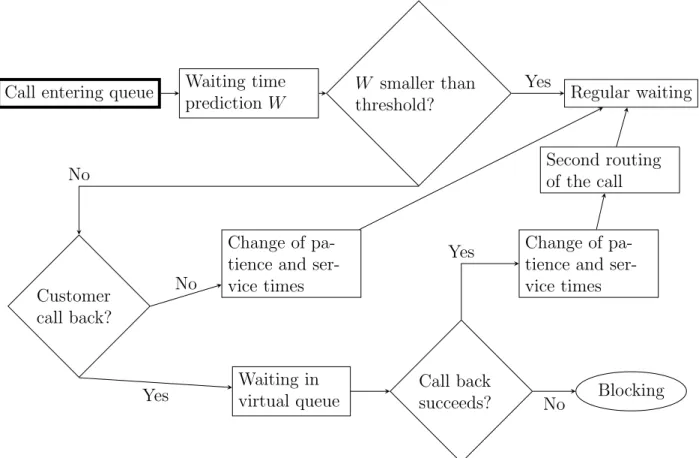
6 Virtual queueing of a call . . . 12

(8)

Listings

1 singleQueue.xml: Example of parameter file for a call center with a single queue . . . 17 2 repSimParams.xml: Example of a parameter file for an experiment using

independent replications . . . 22 3 singleQueueTwoTypes.xml: Example of a parameter file for a call center with

a single agent group and two call types . . . 26 4 singleQueueTwoGroups.xml: Example of a parameter file for a call center

with two agent groups and a single call type . . . 28 5 singleQueueShifts.xml: Example of a parameter file for a call center with

a single agent group with a schedule, and a single call type . . . 30 6 singleQueueMLE.xml: Example of a parameter file with data for parameter

estimation . . . 32 7 repSimParamsTr.xml: Example of a parameter file for an experiment using

independent replications and producing a call-by-call trace . . . 34 8 repSimParamsStat.xml: Example of a parameter file for an experiment using

independent replications and producing a report with selected statistics . . . 34 9 repSimParamsObs.xml: Example of a parameter file for an experiment using

independent replications and producing a report with selected lists of obser-vations . . . 35 10 repSimParamsSeed.xml: Example of a parameter file for an experiment using

independent replications and different initial seed . . . 36 11 repSimParamsSeqSamp.xml: Example of a parameter file for an experiment

using independent replications and sequential sampling . . . 37 12 repSimParamsCTMC.xml: Example of a parameter file for an experiment using

independent replications and CTMC simulator . . . 37 13 mskccParamsThreeTypes.xml: Example of a parameter file for a multi-skill

stationary call center . . . 38 14 batchSimParams.xml: Example of a parameter file for a stationary simulation 40 15 sim2skill.xml: Example of a parameter file for a call center with longest

weighted waiting time router . . . 42 16 mskccParamsThreeTypesReg.xml: Example of a parameter file for a call

cen-ter with local-specialist roucen-ter . . . 46 17 Parameters for the local-specialist routing policy with type-to-group map

equivalent to example in Listing 16 . . . 51 18 Parameters for the agents’ preference-based routing policy with delays

(9)

March 17, 2014 LISTINGS

1

19 op-singleQueue.xml: Example of a configuration file using the OVERFLOW-ANDPRIORITY routing policy giving priority to a call type over the other one . 54 20 Part of op-singleQueue-cp.xml: routing parameters for an example of

pri-orities of calls evolving with waiting time . . . 56 21 op-twoQueues.xml: Example of a configuration file using the

OVERFLOWAND-PRIORITY routing policy, with two call types and agent groups . . . 58 22 Part of op-twoQueues-slowOv.xml: parameters of a routing policy including

routing delays and transfer times . . . 61 23 Part of op-twoQueues-cond.xml: example of parameters for conditional routing 63 24 Part of op-twoQueues-condStat.xml: example of parameters for conditional

routing depending on the service level observed during the last 5 minutes . . 64 25 mskBlendSim.xml: Example of a parameter file for a blend call center . . . . 66 26 mskInOutSim.xml: Example of a parameter file for a blend and multi-skill

call center . . . 69 27 Dialer producing two call types, and using limits . . . 73 28 callTransfers.xml: Example of a parameter file for a model with call transfers 74 29 vq.xml: Example of a parameter file for a model with virtual queueing . . . 77 30 Sample output of the simulator . . . 80 31 CallSim.java: calling the simulator to extract the service level . . . 86 32 Part of CallSimSL.java: obtaining service level estimates for each call type

and acceptable waiting time . . . 87 33 CallSimExport.java: calling the simulator to export results . . . 88 34 CallSimObs.java: calling the simulator to extract observations . . . 90 35 CallSimListener.java: tracking the progress of a call center simulator . . . 91 36 CallSimSubgradient.java: estimating a subgradient . . . 94 37 TestCRN.java: estimating a difference with CRNs . . . 97 38 GetParams.java: getting the arrival rates, service rates, and staffing vector . 100 39 CreateParams.java: creating an instance of CallCenterParams from scratch 102 40 SimulateScenarios.java: simulating scenarios for sensitivity analysis . . . 106 41 WriteSummary.java: simple program writing summary results for different

scenarios . . . 110 42 SimulateScenariosThreads.java: simulate scenarios with multiple threads 113 43 WaitingTimeHistogram.java: program constructing a histogram for the

waiting time distribution . . . 118 44 ExpKernelDensityGen.java: random variate generator using kernel density

with a Gaussian kernel . . . 123 45 Sim2SkillRouter.java: simulation program using a custom router . . . 124

(10)

Part I

Tutorial

1

Overview

A contact center is a set of resources (communication equipment, employees, computers, etc.) providing an interface between customers and a business [16, 7, 4, 1]. Each contact

represents a customer reaching the contact center to obtain some form of service. The service is made by employees in the contact centers calledagents. Each agent is a member of anagent group which determines its characteristics (skills, speed of service, etc.). When a contact cannot be served immediately, it is put in a waiting queue to be served later. The contact center components are linked together by a router which decides on how to assign calls to agents. A call center is a special form of contact center where each contact corresponds to a telephone call.

The ContactCenters library is built using the Java programming language [8] and the Stochastic Simulation in Java (SSJ) library [14], and permits one to implement simulators for contact centers. The library provides building blocks such as classes representing the contacts in the center, the agent groups, the waiting queues, and the router. The programmer combines these blocks to make a simulator. However, creating a simulator directly using this library involves Java programming.

This document presents a ready-to-use generic simulator for the particular case of a blend and multi-skill call center with multiple call types, agent groups and simulation periods. It can simulateinbound calls arriving in the system following a stochastic arrival process as well as outbound calls made by predictive dialers. Service and patience times are also random, and come from any probability distribution supported by SSJ, and parameters can change from time periods to periods.

This simulator is configured through XML files. Compilation of Java code is not required, except if the simulator has to be extended, or used internally by another program. Any XML document intended to be processed by a program conforms to a schema. The simulator uses one such schema for the parameters of the simulated model, and a second schema for the parameters of the experiment method.

The rest of this document is organized as follows. In the next section, we present the call center model implemented by the generic simulator. We define the structure of possible call centers as well as the supported types of experiments. Section 3 introduces the format of the configuration files for the simulator by some commented examples. This is a good way to learn how to make configuration files, not a reference documentation. Section 4 demonstrates how to run the simulator from the command-line while section 5 shows how to interact with the simulator from a Java program. Section 6 discusses most common problems encountered when using the simulator. The last sections contain a reference manual providing detailed documentation for each supported performance measure, routing policies, dialing policies, arrival processes, the supported types of experiments, and the format of generated reports.

(11)

March 17, 2014

3

Section 8 gives a primer on XML, and the data types used in the parameter files. It also gives some examples on how parameter-specific documentation, which is available in HTML only, can be retrieved. The documentation for each parameter was generated from the annotations in the corresponding XML schemas, and can be located in thedoc/schemas subdirectory of ContactCenters.

(12)

2

Simulation model

This section gives a description of the model implemented by the simulator, without ref-erences to specific parameter names in the XML configuration file. See the next section for example configuration files, section 8 for a primer on XML and the data types used in parameter files, and the HTML documentation of the XML Schemas of ContactCenters for more information on parameter names.

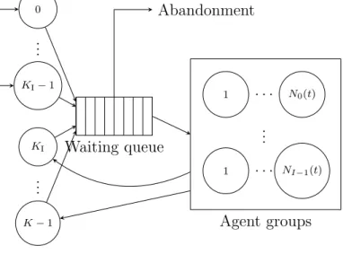
Figure 1 gives an overview of the model implemented by the simulator. It shows that calls are partitioned intoK call types and are sent to agents partitioned intoI agent groups. Inbound calls arrive in the center from external sources while outbound calls are produced by predictive dialers which are part of the call center. Calls that cannot be served immediately are queued, and abandon if they cannot get service after a certain patience time. However, the model is more complex than the figure shows: the queueing discipline is not always first-in first-out, routing can consider agents with multiple skills, and parameters can change during the day. The next sections will examine these aspects in more details.

1 . . . N0(t) .. . 1 . . . NI−1(t) Agent groups Waiting queue 0 KI−1 .. . KI K−1 .. . Contact types Abandonment

Figure 1: The Implemented Model of Call Center

2.1

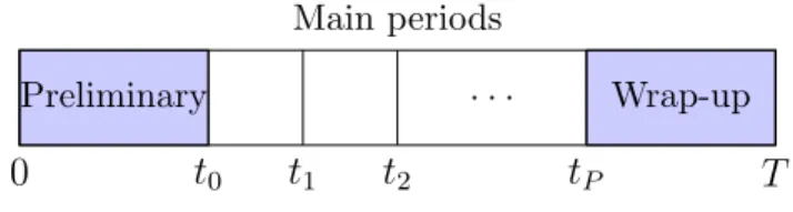
The simulation horizon divided into periods

The simulation horizon can correspond to a day, a week, a month, etc. As shown on figure 2, it is divided intoP+2 time intervals calledperiods. The call center’s opening hours are divided intoP main periods with fixed durationd. For example, these periods may correspond to half hours or hours in the simulated horizon. Main period p= 1, . . . , P corresponds to the time interval [tp−1, tp), where 0≤t0 <· · ·< tP. During the preliminary period [0, t0), no agent is

available to serve calls but arrivals can start a few minutes before t0 for a queue to build up.

During thewrap-up period [tP, T], whereT is the time at which the simulation ends and the

(13)

March 17, 2014 2.2 The processing of a call

5

0 t0 t1 t2 tP T

Preliminary . . . Wrap-up Main periods

Figure 2: The simulated horizon

Parameters are usually specified for the main periods only. During the preliminary period, there are no agents to serve calls and if other parameters are needed, the simulator takes them from the first main period. During the wrap-up period, the parameters from the last main period are used. The preliminary and wrap-up periods can have a length of 0 in several models. They are useful to simulate one day starting where t0 > 0. Since the preliminary

and wrap-up periods are secondary, main periods are often denoted as the periods in the rest of this document.

2.2

The processing of a call

The set ofK call types is divided into two subsets: KI≤K inbound call types with indices

0, . . . , KI−1, and KO outbound call types with indices KI, . . . , K −1. Each call type can

have its owncall source which produces only calls of this type, and can be shut up and down at any time during the simulation. In addition, call sources producing calls of multiple, randomly-chosen types, can be defined. In the latter case, if a call is generated during main period p, its type is k with a fixed probability pk,p, independently of other calls. The way

calls are produced depends on whether they are inbound or outbound, and will be covered in the next subsections.

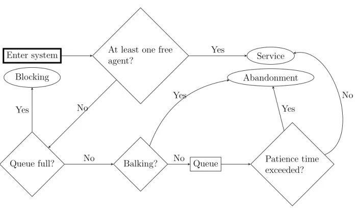
Figure 3 shows the path of a call into the call center. On this figure, rectangles represent processing steps for the call while diamonds represent conditional branching. The rectangle with thick lines represents the starting point of the calls in the system. An ellipse denotes an outcome for a call (blocking, service, or abandonment). When a call arrives, a free agent is selected among the I agent groups. The router (see section 2.4) uses the type of the call to determine which agents are allowed to serve the call, and how agents are chosen if several agents are free. If a free agent is found, the call is sent to that agent, and the agent is allocated for a certainservice time. Conditionally on the call type, agent group and period of arrival of the call, service times are i.i.d. and follow any parametric probability distribution supported by SSJ. If no agent is available for a new call, the call is sent to a waiting queue if that does not exceed the total queue capacity. With some probability depending on the call type and the arrival period, independently of other events, the caller entering queue balks, i.e., it abandons immediately. Other calls having to wait go into a queue where they remain until agents are free to serve them. A queued caller can also become impatient, and abandon without service. Patience times are i.i.d. conditional to call type, and arrival period. If the queue is full at the time of a call’s arrival, the call is blocked instead of entering the queue, i.e., the caller receives a busy signal.

(14)

Enter system

Queue full?

At least one free agent?

Balking? Queue Patience time

exceeded? Blocking Service Abandonment Yes No Yes No Yes No Yes No

Figure 3: The path of a call in the call center

An agent finishing a service can disconnect for a random duration before it takes new calls. The probability and duration of disconnecting may depend on the agent group, and the time period. By default, the probability is 0, so no disconnecting occurs.

2.2.1 Inbound calls

Inbound calls are produced using some arrival processes. Such a process generates ran-dom inter-arrival times following some possibly non-stationary distributions, and generates a single call upon each arrival. The most common distribution for inter-arrival times is ex-ponential, which results in a Poisson arrival process. The simulator supports some variants of the Poisson process with time-varying or stochastic arrival rates. See section 8.3 for more details.

2.2.2 Outbound calls

Outbound calls are produced using a predictive dialer which makes outbound calls when certain conditions apply. There can be one dialer for each outbound call type as well as dialers producing outbound calls of multiple, randomly-chosen, types.

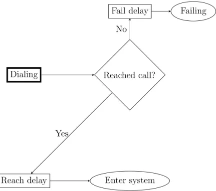
When a dialer is started, it tries to perform outbound calls each time an agent capable of serving calls produced by the dialer becomes free. Each time the dialer is triggered, it decides on how many calls to try, and processes each of these calls independently, as shown

(15)

March 17, 2014 2.3 The agent groups

7

on figure 4. First, dialing succeeds with a reaching probability depending on the call type and period. A delay depending on the success of the call, the call type, and the period of dialing then occurs. The dialing delay can be used to model the party’s phone ringing while a failed call may represent a busy signal, answering machine, etc. Successful calls are processed in a similar way as inbound calls while failed calls simply leave the system after they are counted. During the processing of a successful call, the period of arrival corresponds to the period during which the dialer decided to make a call, not the period during which the call entered the call center.

The only difference when processing inbound calls and successful outbound calls is the service time which includes apreview time that can be used to model the work made by the agent to determine if the right party is reached. The same way as service times, preview times are i.i.d. but can depend on the call type, agent group, and period of arrival. After this preview time, with some probability depending on the call type and period of arrival, the call is a right party connect, and enters regular service. The preview and regular service times are generated independently, and summed up in the case of right party connects. In other words, the time the agent spends with an outbound call is the sum of the preview and service times. On the other hand, if the call is a wrong party connect, it is counted separately and excluded from reports concerning served calls. The service of a wrong party connect only consists of a preview time.

No further special processing is applied to outbound calls in this model. However, some parameters can be adapted to outbound calls. For example, a called customer often balks (or abandons very quickly) if no agent is available to serve him. In fact, any outbound call that needs to wait is called a mismatch, and is avoided in most call centers. Consequently, the average patience time of any outbound call should be small.

The dialer uses a dialer’s policy to determine how many calls to dial each time it is triggered. Let NT

F(t) be the total number of free agents, or equivalently the number of free

agents in thetest set, at simulation timet. Also letND

F,k(t) be the total number of free agents

capable of serving some calls produced by dialerk, or equivalently the number of free agents in thetarget set for dialer k, at simulation timet.

A common dialing condition checks that NT

F(t) ≥ st,k(t), and NF,kD (t) ≥ sd,k(t), where

st,k(t) and sd,k(t) are user-defined thresholds. Their values are constant during periods but

can change from periods to periods. The number of calls to dial at a time is computed from ND

F,k(t) in a way depending on the selected dialing policy. See section 8.4 for more

information.

2.3

The agent groups

Each agent group i has a fixed number Ni(t) of agents at any time during the simulated

horizon. In this model, the functionNi(t) is piecewise-constant. If Ni(t) increases at a given

time t, the additional agents are notified to the router which assigns them queued calls, if possible. The type of the queued call assigned to a new agent in group i depends on the routing policy being used.

(16)

Dialing Reached call?

Fail delay Failing

Reach delay Enter system Yes

No

Figure 4: The path of an outbound call in the call center

Often, agents are added in several groups at a given time t, corresponding, e.g., to the beginning of a main period. In such a case, the router notifies all new agents in group 0 to the router before notifying agents in groups 1, 2, etc. The order in which the agents are notified to the router may have a small impact on which queued calls are assigned to which agent groups, but this only affects a few calls.

IfNi(t) decreases at a given timet, no particular event happens, except ifNi(t) becomes

smaller than NB,i(t). The behavior of the system when that occurs depends on how the

agent group is modeled, but an agent always terminates its on-going service before it can leave.

Only a fraction of the available agents is allowed to serve calls. If there is no busy agent, the total number of agents free to serve calls is given by iNi(t) rounded to the nearest

integer, wherei ∈[0,1] is theefficiency of the agent group. If i = 1, all agents are allowed

to serve calls.

Agent groups can be modeled two ways by the simulator: with counters representing the number of agents in each state, or with entities representing each individual agent. With the first model, the agent group only retains the number of agents which are busy, free, and idle but unavailable to serve calls. When Ni(t)< NB,i(t), on-going services are finished, and

the group does not accept any call until NB,i(t)< Ni(t). However, in the second model, the

so-called detailed group is composed of separate agents with their own states. In that case, when Ni(t) < NB,i(t), some agents are marked to leave the system, but other busy agents

might finish their services before these marked agents leave. As a result, a detailed group can accept new calls even when NB,i(t) > Ni(t). Which agents are marked is not relevant,

(17)

March 17, 2014 2.4 The router

9

and allow for computing the longest idle time of agents, which is needed by some routing policies. However, using counter-based agent groups can increase performance compared to detailed groups.

The Ni(t) functions can be specified three ways: with a staffing vector, with a schedule,

or with individual agents. In the first setting, Ni(t) remains constant during individual

periods. When specifying a schedule, one gives a set of shifts with arbitrary starting and ending times, and assigns some agents to each shift. With the third mode, one assigns each individual agent any user-defined properties in addition to a shift.

2.4

The router

A router assigns agents to inbound calls and successful outbound calls (agent selection or

push routing), and queued calls to free agents (call selection orpull routing), using a routing policy to take its decisions. The model supports a set of predefined routing policies (see section 8.5) that can be parametrized by the user.

The waiting queue represented on figure 1 is partitioned into several elementary waiting queues implemented as lists. The number of waiting queues, and the way they are used depends on the routing policy. Most routing policies assign a waiting queue to each contact type, and all policies supported by the simulator use a First In First Out (FIFO) discipline in individual queues.

Parameters for the routing policy are encoded in one of the three main data structures: a set of ordered lists, incidence matrices, or matrices of ranks. When the first structure is used, thetype-to-group map defines an ordered list of agent groupsik,0, ik,1, . . . for each call typek.

These lists give the order in which agent groups are tested during agent selection. The

group-to-type map defines an ordered list of call types ki,0, ki,1, . . . for each agent group i.

These lists are used during call selection to determine the order in which call types are tested. These routing tables are represented by non-rectangular 2D arrays of integers. In the type-to-group map, there is one row for each call type whereas in the group-to-type map, there is one row per agent group. Any negative integer in these 2D arrays being ignored, they can be used for padding. For an example of a routing policy using this structure, see QUEUEPRIORITYin section 8.5.

The second possible structure is a pair of incidence matrices. Thetype-to-group incidence matrix defines a boolean function iTG(k, i) which determines if calls of typek can be routed

to agents in groupi. The group-to-type incidence matrix defines a similar function iGT(i, k)

that determines if a call of type k can be selected by a free agent in group i. Often, iTG(k, i) =iGT(i, k), i.e., a call of type k can be sent to an agent in group i if and only if a

free agent in groupi can select a call of type k. These matrices are encoded into 2D arrays of booleans. This structure is not used by any router at this moment.

When the third structure is used, the matrices of ranks, which can also be named the priority matrices, define functions rTG(k, i) and rGT(i, k) giving the rank, i.e., priority, of

agents in groupi for calls of type k. The lower the rank, the higher is the preference of the call type k for the agents in group i. When a rank is ∞, calls of type k cannot be served

(18)

by agents in group i. The matrix defining the type-to-group ranks rTG(k, i), specifies how

contacts prefer agents, and is used for agent selection. On the other hand, the second matrix defining the group-to-type ranks rGT(i, k) specifies how agents prefer contacts, and is used

for contact selection. In many cases, it is possible to have rGT(i, k) = rTG(k, i) and specify

a single matrix of ranks. These functions are encoded into rectangular 2D arrays of integers containing, in the case of agent selection, one row for each contact type and one column for each agent group. For contact selection matrices of ranks, the roles of rows and columns are inverted. Although this structure is more flexible than ordered lists, it is often less intuitive to figure out the implied routing. For an example of a routing policy using this structure, seeAGENTSPREF in section 8.5.

Routers using matrices of ranks often use complementary matrices of weights as well. These are similar to matrices of ranks, except they define wTG(k, i) and wGT(i, k) functions

which are weights that can also be considered as penalties. These matrices default to matrices of 1’s if they are not specified.

A last I×K matrix of delays can also be used to specify timers, i.e., d(i, k) gives the minimal time a call of type k must wait before it can be served by an agent in group i.

2.5

Call transfers

The model also supports transfers of calls from agents to agents, i.e., aprimary agent serving a call can transfer the call to a secondary agent. The agent transferring the call can either hang up immediately after the transfer is initiated, or wait for the transfer to succeed or fail. A transfer succeeds when a secondary agent can be assigned to the call, and fails if the call abandons before getting a secondary agent. The transfer process is summarized on figure 5. More specifically, transfer works as follows. Let C be a call of type k arrived during periodp, and served by an agentA in groupi. With probability rk,i,p, the call is transferred

to another agent after service. In that case, we suppose that the transfer decision is taken before beginning of service, and multiply the service time of the call to be transferred by mk,i,p, a constant depending on the call type, group of the serving agent, and main period

of arrival of the call. Let k0 be the target random call type associated with call C for the transfer. This new type index is generated randomly from a discrete distribution giving call type k0 a probability wk,p0_,k0 depending on k and p0.

A new call of typek0 is created, and receives completely new attributes such as patience, and service times. This new callC0 is a virtual call corresponding to C.

A random delay depending on k,i, and pthen occurs. This delay, which is 0 by default, represents the time spent by the agentAto initiate the transfer, e.g., dialing a phone number. After the delay, the new call C0 is sent to the router the same way as an ordinary call. The router’s policy can thus apply specific rules for type k0, which can differ from call typek.

Then, with probability 1−qk,i,p, the agent A is freed although the transfer of the call is

not finished; this is sometimes called a cold transfer. On the other hand, with probability qk,i,p, agent A waits for call C0 to reach a free secondary agent B, or abandons; this is often

(19)

March 17, 2014 2.5 Call transfers

11

End of regular service Transfer? Service

New virtual call Transfer delay Wait for sec-ondary agent? Free primary agent if still busy Routing of vir-tual call Secondary agent found? Conference with primary agent (if still busy) Service with secondary agent Abandonment Yes No No For primary call

Yes

No

(20)

denoted awarm transfer. In case of abandonment, calls C and C0 end, and agentAis freed. Note that call C is counted as a served call, even though C0 abandons.

If service of call C0 begins, and agent A is still waiting, a random conference time de-pending on type k0, period of transfer p0, and secondary agent groupi0 is generated. If this conference time is greater than 0, it adds up to the regular service time of callC0 (i.e., service time is increased), and agentAwaits for the conference time. Note that the conference time is part of the service time both for call C, and call C0.

If service of call C0 begins, but agentA is not waiting, another random pre-service time occurs before the regular service time. This time can be used to model, e.g., a customer identification process.

2.6

Virtual queueing or call backs

Some call centers make predictions of the waiting time of new customers, and offer them the possibility to be called back at a later time if the predicted waiting time is too long. We also say that customers to be called back join a virtual queue since the system must keep a record of such customers in order to perform the callbacks. Virtual queueing is modeled as shown on figure 6 in the simulator.

Call entering queue Waiting time prediction W

W smaller than

threshold? Regular waiting

Customer call back?

Change of pa-tience and ser-vice times Waiting in virtual queue Call back succeeds? Blocking Change of pa-tience and ser-vice times Second routing of the call Yes No No Yes _No Yes

(21)

March 17, 2014 2.7 Simulation experiments

13

More specifically, virtual queueing is allowed for a given call type k by setting a target type index k0 as well as a threshold for the expected waiting time. The index k0 is used to separate calls waiting in regular queue from calls sent to a virtual queue while the threshold is used to test if the predicted queueing delay is sufficiently long for virtual queueing to be worthwhile. When a call whose type allows virtual queueing arrives, an estimate of its expected waiting time is obtained, using the last observed waiting time before a service as a default heuristic. If this prediction W is smaller than a user-defined threshold Wk,p, where

pis the index of the main period of the call’s arrival, the call is processed normally.

Otherwise, with probabilitypk,p, the call exits the regular queue, and is sent to the virtual

queue. This models the fact that the center announces the predicted waiting time to the caller, and the caller chooses to hang up and be called back at a later time. The customer stays in the virtual queue for a fixed time given by W mk,p, where mk,p is a user-defined

multiplier defaulting to 1. With probability 1− pk,p, the customer refuses to be called

back, and waits in the normal queue. However, the patience and service times of such a customer is multiplied by user-defined factors fk,p and gk,i,p, respectively, which default to

1. For example, a patience time multiplier greater than 1 can be used to model the fact that customers knowing their expected waiting time could be more patient than customers ignoring that information.

Before a call enters the virtual queue, its type identifier switches fromk tok0. When the customer leaves the virtual queue, call back occurs: with probabilityck,p, call back succeeds

and the call is sent back to the router to get a free agent, or to be queued again, hopefully for a smaller time than if the customer had waited on the phone. Of course, the parameters of the routing policy can be different for call types k and k0. For example, calls of type k0 often have priority over calls of typek. With probability 1−ck,p, call back fails and the call

returning from the virtual queue is lost; it is counted as a blocked call in statistical reports. Note that any random variable associated with the call having switched type for virtual queueing is not generated a second time, from the distribution corresponding to type k0; the original values for call typek are kept. However, the patience and service times of calls returning from virtual queue are multiplied by factorshk,p, and ik,i,p, respectively. This can

be used, e.g., to model the fact that called back customers are not ready to wait as long as regular customers.

2.7

Simulation experiments

Once the model parameters are set up, the simulator can perform experiments whose aim is to estimate performance measures corresponding to expectations or functions of expectations. Estimation is made using averages, or functions of averages, respectively.

Usually, one simulates the complete horizon of the model, and collects the resulting estimates. The experiment is repeated several times with different random numbers in order to i.i.d. observations for computing averages, functions of averages, confidence intervals, etc., for estimated performance measures. Without multiple replications, the estimators would be too noisy to be useful.

(22)

Alternatively, one can concentrate on a single period of the horizon, and simulate it as if its duration was infinite in the model. The parameters of the model are then fixed for the whole simulation, and the system is simulated for a certain time, usually larger than the duration of the considered period. The simulator uses batch means [13, 5] to compute confidence intervals on performance measures. See section 9 for more details about these two types of experiments.

2.8

Simulation output

After any experiment, the simulator generates a report containing general information as well as statistics for estimated performance measures. More specifically, the simulator computes many (random) quantities on (constant) time intervals [t1, t2] such as the number of calls

processed by the router (arrived calls), the number of served and blocked calls, calls which have abandoned, etc. It also evaluates the integrals of the number of busy and working agents over the interval [t1, t2], for each agent group. The time interval can be the whole simulation,

a single period, etc., and statistics may be computed for several different intervals.

By default, a call arriving during periodpis counted in statistics related to periodp, even if it exits the system during period p+ 1. However, using the perPeriodCollectingMode attribute in experiment parameters, one can make the simulator count the calls in the period they leave the system.

Statistics are collected for main periods only. As a consequence, if the statistical period of a call is the preliminary or wrap-up period, the call is not counted. Without this restriction, the time interval of a statistic on the whole horizon would be random, and could change from replications to replications.

Usually, a call is counted once. If a call switches from typektok0 due to virtual queueing, it is counted as a type-k0 call when call back fails, or at abandonment or end-service time. However, when a call is transferred to another agent, the call served with the primary agent is counted separately from the virtual call produced by the transfer.

A performance measure on a time interval [t1, t2] can concern a segment of call typesk,

a segment of agent groups i, or a pair (k, i). Here, a segment is simply a set regrouping call types or agent groups. LetK0 be the number of segments of call types. For more information about segments, see sections 10.3 to 10.5.

Random variables concerning a fixed time interval can be regrouped into a random vector X(t1, t2)∈ Rd. The expectation E[X(t1, t2)] is a vector of d possible performance measures

which can be estimated by a vector of averages ¯Xn(t1, t2).

Other performance measures can be defined using functions g : _Rd → _R, and corre-spond to functions of expectations g(_E[X(t1, t2)]) estimated using functions of averages

g( ¯Xn(t1, t2)). For example, by dividing the average sum of waiting times by the average

number of arrivals, we obtain the long term average waiting time over all calls which esti-mates the long term expected waiting time. Dividing the average number of busy agents by the average number of agents gives the long term agents’ occupancy ratio.

(23)

March 17, 2014 2.9 The simplified CTMC model

15

Another important performance measure is the service level defined as follows. Let SG,k,p(sk,p) be the number of contacts served after a waiting time less than or equal to sk,p,

in inbound type segment k, and counted in period segment p. Let Sk,p be the total number

of served contacts in inbound type segmentkcounted in period segmentp. The constantsk,p

is the acceptable waiting time, and can depend on k = 0, . . . , K_I0−1 and p= 0, . . . , P0 −1. Also letLG,k,p(sk,p) be the number of contacts in inbound type segmentk, counted in period

segmentp, and having abandoned after a waiting time smaller than or equal to the acceptable waiting time, andAk,pbe the total number of arrivals, for inbound type segmentk, and period

segment p. The service level for inbound type segmentk, and period segment p is defined as

g1,k,p(sk,p) = E

[SG,k,p(sk,p)]

E[Ak,p−LG,k,p(sk,p)]

. Other definitions are possible for the service level, e.g.

g2,k,p(sk,p) = E

[SG,k,p(sk,p) +LG,k,p(sk,p)]

E[Ak,p]

.

To make reporting easier, related performance measures are regrouped into matrices whose rows represent segments of contact types or agent groups, and whose columns usually represent time intervals. In some situations, there is a single period, which results in single-column matrices. For example, the expected number of served calls of each type, and for each period, estimated by averages, is such a group of performance measures.

Many other performance measures can be estimated by the simulator. See section 10.3 for a complete list of supported performance measures. See also section 10 for more information about how confidence intervals are computed, and the contents and possible formats of statistical reports.

2.9

The simplified CTMC model

Simulation-based optimization requires many replications to evaluate the performance of a call center for different configurations, e.g., with different staffing vectors. With the generic multi-skill and blend simulator using the model described here, this is often too CPU inten-sive. The commonly used approximation formulas to work around this problem oversimplify reality. An alternative simulator using a simplified continuous-time Markov chain (CTMC) model is thus provided. This simulator generates transitions using the embedded discrete-time Markov chain (DTMC), and computes expectations conditional to the sequence of visited states.

The CTMC model used by this simulator is similar to the model described in this section, with the following simplifications. First, arrivals always follow the Poisson process, patience and times are exponential, there is no outbound call, no virtual queueing, no call transfer, and agents cannot disconnect after service termination. Moreover, the queue capacity is always finite.

(24)

The following routing policy is used to select an agent for a new call. Each call type k has a list Ik,0, Ik,1, . . ., where Ik,j is a set of agent groups, for j = 0, . . .. When a call of

type k arrives, if at least one free agent is available in one of the groups in Ik,0, the call is

sent to a free agent in the group of Ik,0 containing the greatest number of free agents. If

several groups i∈Ik,0 contain the same maximal number of free agents, the group with the

maximal number of free agents, and the smallest index i is taken. On the other hand, if no group in Ik,0 contains free agents, the sets Ik,1, ik,2, etc. are tested in a way similar to Ik,0,

in the order given by the list, to choose the first set with an agent group containing at least one free agent. The setsIk,j are constructed from the matrix of ranks given by the user. In

particular, the set Ik,0 is constructed by taking each agent group i with the minimal rank

rTG(k, i). The set Ik,1 is created by taking groups i with second smallest rankrTG(k, i).

For the selection of call at the end of service, each agent group has a list Ki,0, Ki,1, . . . of

sets of call types. First, if one waiting queue in Ki,0 contains at least one call, the service

starts for the call having spent the greatest number of DTMC transitions in queue, among calls in queues of Ki,0. If more than one call spent the greatest number of transitions in

queue, the call with the greatest number of transitions in queue and the smallest index k is taken. On the other hand, if no queue in Ki,0 contains calls, the sets Ki,1, Ki,2, etc. are

checked in a way similar to Ki,0, in the order given by the list, to find the first set with

a queued call. In a way similar to Ik,j, the sets Ki,j are constructed by using the values

(25)

March 17, 2014

17

3

Examples of data files

The configuration of the simulator is specified by at least two XML files. A XML [21] file contains a hierarchical structure of elements with possible attributes and nested contents. An overview of XML and data structures supported by the simulator is provided in Section 8.1. The first file specifies the parameters for the call center itself. These parameters are usually determined by a manager based on a real system. The second file specifies parameters for the simulation experiment, such as the simulation length, the required target relative error, etc. These parameters are determined by the simulation expert at the time experiments are performed. Two formats are available for encoding parameters describing experiments: a first one for the batch means method and a second one for simulation using independent replications.

In this section, we present examples of parameter files for different models of call centers. We start with a single queue, and extend it by adding a new call type, a new agent group, etc. The last examples are blend call centers with one inbound call type and one outbound call type. The last example is a blend and multi-skill call center demonstrating most of the possibilities of the simulator.

3.1

Single queue

This example models a call center with a single call type, a single agent group, but multiple time periods. Each day, the center operates forP hours. The parameters can change during the day, but they are constant within each hour.

Calls arrive following a Poisson process with piecewise-constant arrival rate λp during

periodp, where λp is constant. Calls that cannot be served immediately are put in a FIFO

queue, and abandon if they wait more than their patience time. The i.i.d. patience times are generated as follows: with probabilityρ, the patience time is 0, i.e., the caller abandons if he cannot be served immediately. With probability 1−ρ, the patience time is exponential with mean 1/ν. Service times are i.i.d. exponential random variables with mean 1/µ.

During main period p, Np agents are available to serve calls. If, at the end of period p,

the number of busy agents is larger thanNp+1, ongoing calls are completed, but new calls are

not accepted until the number of busy agents is smaller than Np+1. During the preliminary

period, there is no agent whereas for the wrap-up period, NP+1 = NP. Listing 1 presents

the XML file for this example.

Listing 1: singleQueue.xml: Example of parameter file for a call center with a single queue <ccmsk:MSKCCParams defaultUnit="SECOND" periodDuration="PT1H"

numPeriods="13" startingTime="PT8H"

xmlns:ccmsk="http://www.iro.umontreal.ca/lecuyer/contactcenters/msk"> <inboundType name="Inbound Type">

(26)

</serviceTime>

</inboundType>

The XML file presented here is composed of elements and attributes describing the hierar-chical data. In a XML document,elements are used to represent complex data. Each element has a tag name, e.g., serviceTime, opening and closing markers (e.g., <serviceTime>, and </serviceTime>), a set of attributes, and nested contents. An attribute is a key-value pair representing simple data associated to an element while nested contents can be simple text or children elements. Each document has a single root element which can have an arbitrary number of attributes and children. See Section 8 for more information. The elements of

(27)

March 17, 2014 3.1 Single queue

19

any XML document can be represented as a tree such as the one displayed on figure 7. The figure shows thatMSKCCParamsis the root of the tree, and has one child for the inbound call type, one child for the agent group, etc. We now describe the XML file in more details.

MSKCCParams inboundType probAbandon patienceTime serviceTime arrivalProcess agentGroup staffing router ranksTG routingTableSources serviceLevel awt target

Figure 7: The hierarchical structure of example in Listing 1

For call center parameters, the name of the root element must be MSKCCParams with a namespace URI set to http://www.iro.umontreal.ca/lecuyer/contactcenters/msk. The xmlns:ccmsk attribute of this root element is used to bind this URI to the shorter prefix ccmsk in the parameter file.

The root element is allowed to have some attributes such as periodDuration (main period duration d), defaultUnit (default time unit), etc., as well as children elements. The attributes of an element are given after the name of the element, and before the > marker. Nested contents of the root element is located between the <ccmsk:MSKCCParams> and </ccmsk:MSKCCParams>markers.

In this model, 13 periods of one hour are set up by settingnumPeriodsto 13 and period-Durationto PT1H. The notation for time durations, which seems confusing at first sight, is

(28)

imposed by the XML Schema Specification (see Section 8.2.1, and [19, part 2, section 3.2.6]). The attribute defaultUnit, set toSECOND in this example, sets the implicit unit for time durations. This is the time unit used during simulation as well as the unit of any time-related output, e.g., waiting time.

Nested elements are used to describe more complex information such as call types, agent groups, the router, and the parameters for estimating the service level. The order of these elements must not be changed for the parameter file to remain valid. It is also important to keep the hierarchy of the document, e.g., the routerelement should not be moved inside an inboundTypeelement.

We now describe the contents of theinboundTypeelement, which represents the call type in this example, in more details. First, the name attribute is used to bind a name to the inbound call type. A name can also be associated with an agent group.

The probAbandonelement is used to set the probability of balking, for each main period. This element accepts an array of values on the [0,1] interval. If the array contains a single value such as in this example, the value is automatically reused for all periods. Therefore, the user does not need to repeat 0.1 13 times to haveρ= 0.1 for all periods in this example. The way patience and service times are specified differ from the way the period dura-tion is given, because these aspects of the model require probability distribudura-tions, not only mean time durations. The distribution for patience time is given using the patienceTime element whose type corresponds to a probability distribution. Such an element accepts a distributionClass attribute giving the SSJ class of the probability distribution while the defaultGenchild element sets the distribution parameters. The latter element accepts an ar-ray giving the arguments passed to the constructor of the chosen distribution class. The role of these arguments depends on the chosen distribution class, and do not always correspond to means and variances.

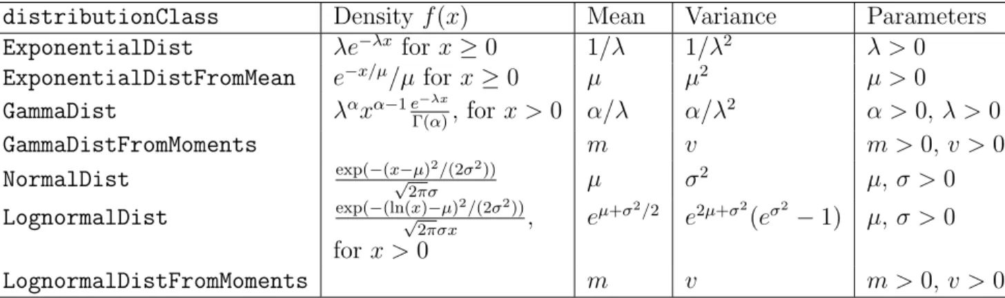
Table 1 gives the parameters for the most commonly used distributions. The first column gives the name of the class, i.e., the value of the distributionClassattribute, correspond-ing to the distribution. The other columns give the density of the distribution, its mean, its variance, and the order of parameters required for the distribution. See the package umontreal.iro.lecuyer.probdistin the user’s manual of SSJ [14] for additional distribu-tions.

According to Table 1 or the SSJ documentation from [14], the exponential distribution is represented by the ExponentialDistFromMean class, and has a scale parameter µ repre-senting the mean which needs to be specified as an argument for calling the constructor. Here, µ= 1000. The unit attribute of patienceTime specifies that the generated patience times must be considered in seconds, so the mean patience time is 1000s for this example. The serviceTimeelement has the same structure aspatienceTime, but it gives the service time distribution for calls, served by any agent.

ThearrivalProcesselement specifies the arrival process to be used for this inbound call type, along with its parameters. The type attribute is used to indicate the type of arrival process, which can be any string specified in Section 8.3. The arrivals vector element gives the parameters for the arrival process, in this case the Poisson arrival rate. By default,

(29)

March 17, 2014 3.1 Single queue

21

Table 1: Parameters for the most commonly used probability distributions

distributionClass Density f(x) Mean Variance Parameters

ExponentialDist λe−λx _for _x_≥₀ ₁_/λ ₁_/λ2 _{λ >}₀

ExponentialDistFromMean e−x/µ_/µ _for _x_≥₀ _µ _µ2 _{µ >}₀ GammaDist λα_xα−1e−λx Γ(α), for x >0 α/λ α/λ 2 _{α >}_0, _{λ >}₀ GammaDistFromMoments m v m >0,v >0 NormalDist exp(−(x√−µ)2/(2σ2)) 2πσ µ σ 2 _µ_, _{σ >}₀ LognormalDist exp(−(ln(x)√ −µ)2/(2σ2)) 2πσx , e µ+σ2_/2 e2µ+σ2 (eσ2 −1) µ, σ >0 for x >0 LognormalDistFromMoments m v m >0,v >0

Here, Γ(α) =R₀∞xα−1_e−x_dx_{. In particular, Γ(}_n_{) = (}_n₋_{1)! when} _n _{is a positive integer.}

The gamma and lognormal distributions with moments have the same density as the ordinary gamma and lognormal distributions, but a mean and a variance are entered rather than shape and scale parameters.

this arrival rate corresponds to the expected number of calls during a simulation time unit, i.e., one second in our setting. By setting the normalize attribute totrue, we instruct the simulator to interpret the arrival rates as relative to one period. Consequently, the given arrival rates set the expected number of arrivals during each hour for this example.

The agentGroup element describes the agent group in the call center. The staffing child element is used to associate a staffing with the agent group. It contains an array giving the number of agents during each main period of the day. Alternatively, the array can contain a single element; the staffing will then be fixed for the whole day.

Then, the agentGroup element is used to describe the agent group of the example. We give a name to the agent group using thename attribute and configure its staffing using the staffingelement. This gives a number of agents for each main period of the model.

The routerelement is then used to describe how routing is done in the model. Here, we have a very basic routing sending any incoming call to a free agent. For this, the router-Policy attribute is used to configure the router’s policy. Here, we use the AGENTSPREF policy which is very general. But we could use other more efficient policies for this example. Section 8.5 describes in details the available router’s policies.

The selected router’s policy minimally requires a K×I matrix associating a priority to each (call type, agent group) pair during agent selection, and a secondI×K matrix setting the priorities similarly during call selection. The first matrix is set usingranksTG(ranks for type-to-group assignments) while the second matrix is given usingranksGT(ranks for group-to-type assignments). A matrix can be represented by a sequence of arrays in the parameter file, each array being represented by a row child element. Here, we use the 1×1 identity matrix for both parameters. The second matrix can be given explicitly using the ranksGT. However, instead of transposing the contents of ranksTGmanually to obtainranksGT when

(30)

rTG(k, i) = rGT(i, k) for all k and i, we can instruct the router to generate ranksGT by

transposing ranksTG, by using theroutingTableSources element. This will become useful when we increase the number of call types and agent groups.

The serviceLevelelement gives thresholds for the service level using two K_I0 ×P0 ma-trices: one for the acceptable waiting times, and a second one for the service level targets. Often, K_I0 =KI+ 1 ifKI >1, and KIotherwise, and P0 is defined similarly usingP. Several

serviceLevel elements, with different awt and target matrices, can be specified to set the values for different contact types and periods. The targets are not considered during simulation, but they can be used by optimization programs.

However, these matrices are sometimes sparse, i.e., the user only specifies some values. Consequently, if a matrix of thresholds (or targets) contains a single element, its single value is used for all call types and periods. If it contains a single row or column, the row or column is duplicated as required.

Here, we set the acceptable waiting time to 20s, and the service level target to 80%. We need 1×1 matrix containing PT20S, and 0.8, respectively. We also specify a second threshold of 30s with target 80% by using a second serviceLevelelement.

After the model parameters are configured, simulation parameters are needed in order to perform experiments. The simplest method of experiment consists of simulating a fixed number of independent replications. This can be described by a file similar to Listing 2.

Listing 2: repSimParams.xml: Example of a parameter file for an experiment using inde-pendent replications

<ccapp:repSimParams minReplications="100"

xmlns:ccapp="http://www.iro.umontreal.ca/lecuyer/contactcenters/app"> <report confidenceLevel="0.95"/>

</ccapp:repSimParams>

The root element for the parameter file is repSimParams with namespace URIhttp:// www.iro.umontreal.ca/lecuyer/contactcenters/app, which differs from the namespace URI ofMSKCCParams. The number of performed runs is fixed to 300 by theminReplications attribute.

The report element contains the parameters of the statistical report produced by the simulator. In particular, theconfidenceLevelattribute sets the confidence level of intervals to 95%. These confidence intervals are computed using the normal assumption (see Section 10 for more details). The report is printed when the simulator is invoked from the command-line or when the formatStatistics method is called from a Java program. This includes the confidence level of the printed intervals as well as the statistics to include in the report. Here, no information is provided about printed statistics so the report includes information about all supported performance measures.

(31)

March 17, 2014 3.2 Variants of the single-queue model

23

3.2

Variants of the single-queue model

3.2.1 Disabling abandonment

In some situations, it can be necessary to disable abandonment, e.g., if no information about patience is available, or if simulation needs to be compared with approximation formulas. Doing this increases the workload of the simulated agents, because customers abandoning must now all be served. This increases the waiting time, and decreases the service level if the number of agents is not increased to compensate for this. Of course, a model without abandonment is less realistic than an equivalent model with abandonment.

Abandonment can be disabled by removing probAbandon and patienceTime from the XML file. Removing probAbandondisables balking by setting the probability of immediate abandonment to 0 while removing patienceTimesets all patience times to infinity.

Removing an element from a XML file can be performed by destructively deleting all the text representing the element, and its children, or by commenting it out. For example, the following code represents a patience time which was commented out:

<!

--<patienceTime distributionClass="ExponentialDistFromMean" unit="SECOND"> <defaultGen>1000</defaultGen>

</patienceTime>

-->

The sequences serve as comment delimiters in the XML language. Since com-ments are ignored by the parameter reader, they can be used to store additional information about the parameter file. This information is intended to be used by human beings only. Any information used by a computer program should be encoded in XML elements, attributes, or nested text.

3.2.2 Setting period-specific parameters

The example on Listing 1 sets a stationary distribution for the patience and service times. If the distribution of the service times can change from periods to periods, one can replace the defaultGenelement of serviceTimewith a sequence of periodGenelements, as shown on the next listing.

(32)

This sets the per-period mean service time, for a model defining five main periods. The pth periodGen element gives the parameters of the service time for main period p, with p= 1, . . . , P. Of course, the number of periodGenelements must correspond to the number of main periods in the model.

3.2.3 Increasing the variability of arrivals

1 _{With the arrival process of the original model, the number of arrivals during period}

p follows the Poisson distribution with mean λp, and variance λp. This variance can be

increased randomizing the arrival rate in each period. The arrival process is then doubly stochastic. For example, this can be done by setting the arrival rates to Bλp, where B is a

random variable with mean 1. The random variable B, generated each day, represents the busyness factor of the day. The day is more busy than usual when B > 1 and less busy than usual when B <1. A well-studied distribution forB is gamma with equal parameters α0 [3]. Such a busyness factor can be used by adding the busynessGenelement before any

inboundTypeelement, e.g.,

This sets the distribution of the busyness factor to gamma(10,10). This element does not acceptdefaultGen orperiodGen children, because the busyness factor is generated once at the beginning of the day, and thus does not change from periods to periods.

Another way of increasing the variance of the number of arrivals is to use a Poisson-gamma arrival process where the arrival rate for each period is gamma-distributed, independently of other periods. This can be specified as follows:

<arrivalProcess type="POISSONGAMMA" normalize="true"> <poissonGammaShape>19 19 19 19 19 19 19 19

19 19 19 19 19</poissonGammaShape> <poissonGammaRate>100 150 150 180 200 150 150 150

120 100 80 70 60</poissonGammaRate> </arrivalProcess>

Here, we have changed the value of the type attribute to POISSONGAMMA, and replaced the arrivals element with poissonGammaShape, and poissonGammaRate. These new elements give the gamma shape and rate parameters for each main period. Section 8.3 gives the list of all available arrival processes, with a detailed description for each one.

1_{From Richard: Le d´}_{ebut de cette section doit ˆ}_{etre r´}_e´_{ecrit pour tenir compte de nos derni`}_{eres corrections:} on peut inclure un facteur busyness pour chaque type d’appel.

(33)

25

3.2.4 Changing the number of periods

Increasing the number of periods often requires several updates in the parameter file. First, the numPeriods attribute in MSKCCParams must be modified. Then, each element defining period-specific parameters must be updated with the new periods. This includes balking probabilities stored inprobAbandonelements, patience and service times stored in patience-Time and serviceTime elements, arrival process (arrivals elements for Poisson processes with piecewise-constant rates), staffing in staffing elements, and service level information inserviceLevelelements. Missing per-period parameters will result in error messages when running the simulator. If an element sets parameters for more periods than the value given bynumPeriods, the last extra periods are ignored.

3.2.5 Adding a new call type

Adding a new call type is a three-steps process: 1. Adding a new inboundType element;

2. Adapting the routing policy for a new call type;

3. Extending the matrices of AWTs and targets for the service level. We now describe these steps in more details.

Adding a new inboundTypeelement can be done by copying the contents of an existing inboundTypeelement, and altering its contents. The main issue to consider is the indexing of call types: adding new call types can shift indices, and require adjustments in other parts of the XML file. More specifically, each call type receives an index based on its order of occurrence in the XML file. This index is used for specifying type-to-group and group-to-type maps for some routing policies as well as target call group-to-types for call transfers and virtual queueing. See Section 3.4 for an example with a type-to-group map.

In our original setting, the only call type has index 0. Adding a new inboundType element just below the original one creates a new call type with index 1. However, adding the element before the original inboundType element assigns index 0 to the new call type, and shifts the index of the old call type to 1. This can cause problems especially if the model already contains several call types.

The second step in adding the call type is to update the parameters of the routing policy. In our example, we need to change the ranksTGchild element of router in order to extend the matrix of ranks with a new row. This new row sets the priorities for the new type. Failing to do that will result in errors preventing the simulator to run.

With a single agent group and the agents’ preference-based routing policy, if both call types have the same priority, agents becoming free select the call with the longest waiting time. Otherwise, free agents first look for calls with the lowest rank (i.e., highest priority) before calls with the highest rank.

(34)

If call type 1 has priority over call type 2, or even if its mean service time is shorter than the mean service time of call type 2, calls of type 1 will wait less before they get service, and therefore will have higher service level than calls of type 2.

If both call types have the same priority, and mean service time, one expects to get exactly the same results as with the model defining a single call type. In practice, results differ slightly because of the way random numbers are generated by the simulator. More specifically, sequences of random numbers are associated to each call type separately. By splitting the calls in two types, one changes the number of constructed sequences of random streams, and thus the generated random numbers. Note that the difference between the single-type and the two-types model decreases as the number of replications increases.

Extending matrices of AWTs and service level targets is optional if it contains a single row, and the thresholds and targets do not depend on the call type. Otherwise, the matrices must contain one row per call type, plus a row for the global parameters.

Listing 3 gives an example of a call center with two call types, and one agent group. Here, the target service level is 80% for both types, but the AWT for call type 2 is set to 60s. The global AWT and target remain at 20s, and 80%, respectively. In the new model, calls of type 1 have priority over calls of type 2.

Listing 3: singleQueueTwoTypes.xml: Example of a parameter file for a call center with a single agent group and two call types

<ccmsk:MSKCCParams defaultUnit="SECOND" periodDuration="PT1H"

numPeriods="13" startingTime="PT8H"

xmlns:ccmsk="http://www.iro.umontreal.ca/lecuyer/contactcenters/msk"> <inboundType name="Inbound Type 1">

</patienceTime>

</serviceTime>

</inboundType>

</patienceTime>

</serviceTime>

(35)

27

</inboundType>