Pepler, P.T.
, Uys, D.W., and Nel, D.G. (2016) Discriminant analysis under
the common principal components model. Communications in Statistics:
Simulation and Computation, (doi:
10.1080/03610918.2015.1134568
)
This is the author’s final accepted version.
There may be differences between this version and the published version.
You are advised to consult the publisher’s version if you wish to cite from
it.
http://eprints.gla.ac.uk/114766/
Deposited on: 22 January 2016
Discriminant analysis under the common principal components
model
P.T. Pepler∗, D.W. Uys†, D.G. Nel†
December 14, 2015
∗Unit for Biometry, Genetics Department, Stellenbosch University (corresponding author) †Department of Statistics and Actuarial Science, Stellenbosch University
Abstract: For two or more populations of which the covariance matrices have a mon set of eigenvectors, but different sets of eigenvalues, the common principal com-ponents (CPC) model is appropriate. Pepler et al. (2015) proposed a regularised CPC covariance matrix estimator and showed that this estimator outperforms the unbiased and pooled estimators in situations where the CPC model is applicable. This paper extends their work to the context of discriminant analysis for two groups, by plug-ging the regularised CPC estimator into the ordinary quadratic discriminant function. Monte Carlo simulation results show that CPC discriminant analysis offers significant improvements in misclassification error rates in certain situations, and at worst performs similar to ordinary quadratic and linear discriminant analysis. Based on these results, CPC discriminant analysis is recommended for situations where the sample size is small compared to the number of variables, in particular for cases where there is uncertainty about the population covariance matrix structures.
Keywords: Common principal components; Discriminant analysis; Covariance matrix; Monte Carlo simulation.
1
Introduction
The common principal components (CPC) model was proposed by Flury (1988) to describe the case where the covariance matrices of several populations have the same set of eigenvectors, but each with a distinct sets of eigenvalues. Formally, the CPC hypothesis can be written as
HCPC:Σi=BΛiB0, i= 1, . . . , k, (1)
where Σi is the covariance matrix of the ith population, Λi is a diagonal matrix containing
the eigenvalues of the ith population covariance matrix on the diagonal, and B is the common eigenvector matrix. The column order ofB need not be the same for all kpopulations.
Pepler et al. (2015) proposed using a regularised covariance matrix estimator under the CPC model to obtain improved covariance matrix estimates, and have shown that this estimator performs well even in cases where the CPC assumption is false. Building on this work, it is of interest to investigate whether these covariance matrix estimators can be used to improve misclassification error rates in discriminant analysis. If there is more accurate information available about the structures of the population covariance matrices, it should be easier to determine to which group a new observation belongs. Plugging the CPC covariance matrix estimators into the quadratic discriminant function leads to what is called the CPC discriminant function, which is introduced in Section 2.
The topic of CPC discriminant analysis was studied by Schmid (1987), with the main results summarised by Flury (1988). Flury and Schmid (1992) derived asymptotic results for discrimina-tion coefficients under homogeneous, propordiscrimina-tional, CPC and unrelated covariance matrix models, respectively. They showed that, although CPC discrimination can improve on the misclassifica-tion rate of ordinary quadratic discriminamisclassifica-tion in some situamisclassifica-tions, such improvement is usually not substantial. They suggested that both the proportional and CPC models can perform well in clas-sification applications where the number of variables and/or number of groups are large relative to the sample sizes, and that these models offer a compromise between the assumption of equal covariance matrices on the one extreme and the assumption of unrelated covariance matrices on the other. For sparse data, theoretically incorrect but more parsimonious models can outperform theoretically correct models in discriminant analysis applications, because the discriminant
func-tion coefficients for a more parsimonious model will generally be less variable (Flury and Schmid, 1992).
Flury et al. (1994) followed up these investigations with a simulation study to determine the misclassification error rates for the different covariance matrix estimators when plugged into the quadratic discriminant function. They showed that CPC discrimination often does not have a great advantage over ordinary quadratic discrimination (using the unbiased sample estimators of the population covariance matrices), and that in many situations the performance of quadratic discrimination under the proportional model compares well with the results achieved by using the linear discriminant rule. They concluded that ordinary quadratic discrimination should be avoided if possible, as it performs poorly in all scenarios except when there are large samples available from populations with unrelated covariance matrices.
Friedman (1989) proposed a technique known as regularised discriminant analysis for high-dimensional, sparse data settings. This method is briefly discussed in Section 3, pointing out a relation to CPC discrimination based on the regularised CPC covariance matrix estimator proposed by Pepler et al. (2015).
Bianco et al. (2008) used partial influence functions to derive the asymptotic variances of the discriminant function coefficients under the same models considered by Flury and Schmid (1992), and their results confirmed the order relations of the coefficient variances from the earlier study. They also performed a simulation study using multivariate normal as well as contaminated data (i.e. a mixture of data from two different normal distributions), and their results confirmed what was found previously by Flury et al. (1994) concerning the performance of the different discriminant functions. The results of the Monte Carlo simulation experiments presented in Section 4 of this paper are compared to these previous studies.
2
Discriminant analysis under the CPC model
Suppose that samples fromk= 2 multivariate normally distributed populations with unequal mean vectors and common covariance matrix, Σ, are available. Indicate the unbiased sample estimators of the mean vector and covariance matrix of the ith population with ¯xi and Si, respectively, and
c= 1 2(¯x 0 1S −1 p x1¯ −x¯ 0 2S −1 p x2¯ ), (2)
where Sp indicates the pooled covariance matrix estimator,
Sp = Pk i=1(ni−1)Si Pk i=1(ni−1) . (3)
Assuming equal costs of misclassification and equal prior probabilities of occurrence, a new observation with unknown group membership status, xnew, is allocated to the first group (i.e.
belonging to the first population) if
(¯x01−x¯02)S−p1xnew≥c, (4)
otherwise it is allocated to the second group. Equation (4) is known as the linear classification rule (Johnson and Wichern, 2002). The purpose of the linear discriminant function is to find the linear combination of thep variables giving the greatest separation between the group centroids in thep-dimensional space.
Fisher (1938) derived the same linear classification rule in (4) without the multivariate normality assumption. The multivariate normality assumption is thus not necessary for linear discriminant analysis (LDA), and the method can also be applied to multivariate non-normal data.
If the assumption of homogeneous covariance matrices for the two populations is untenable, quadratic discriminant analysis (QDA) should be used instead. Unlike the linear discriminant function, the quadratic discriminant function depends on the assumption that the populations have multivariate normal distributions. QDA should therefore not be used if the normality assumption seems doubtful. For samples from k= 2 multivariate normally distributed populations, let
c= 1 2ln | S1| |S2| +1 2(¯x 0 1S−11x¯1−x¯02S−21x¯2). (5)
Assume equal costs of misclassification for the two groups and equal prior probabilities of occurrence. According to the quadratic classification rule, a new observation,xnew, is allocated to
the first group if
−1x0new(S−11−S−21)xnew+ (¯x01S −1 1 −x¯ 0 2S −1 2 )xnew≥c, (6)
otherwise it is allocated to the second group (Johnson and Wichern, 2002).
Under the multivariate normality assumption, more accurate estimators of the population co-variance matrices in (5) and (6) can lead to improved classification rules and lower misclassification error rates. This hypothesis have been investigated by Schmid (1987), Flury (1988), Flury and Schmid (1992), Flury et al. (1994) and Bianco et al. (2008). For CPC discrimination, the unbiased covariance matrix estimators in (5) and (6) are simply replaced by covariance matrix estimators under the CPC model. With ˆB indicating the estimated eigenvector matrix common to all k
population covariance matrices, Flury (1988) proposed
Si(CPC)= ˆBL0iBˆ0, i= 1, . . . , k, (7)
as an estimator of the ith population covariance matrix under the CPC model, where
L0i = diag( ˆB0SiBˆ) (8)
is a diagonalised matrix with the eigenvalues of the ith group (under the CPC model) on the diagonal. Let c= 1 2ln |S 1(CPC)| |S2(CPC)| +1 2(¯x 0 1S−1(CPC)1 x¯1−x¯ 0 2S−2(CPC)1 x¯2), (9)
where S1(CPC) and S2(CPC) are the CPC covariance matrix estimators in (7) for the first and second groups, respectively. Under the CPC assumption, the quadratic discriminant rule becomes: Allocate a new observation,xnew, to the first group if
−1 2x 0 new(S−1(CPC)1 −S −1 2(CPC))xnew+ (¯x 0 1S−1(CPC)1 −x¯ 0 2S−2(CPC)1 )xnew≥c, (10)
otherwise allocate it to the second group. The CPC estimators in (9) and (10) can also be replaced by the regularised CPC estimators proposed by Pepler et al. (2015), i.e.
S?i(CPC)=αiSi+ (1−αi)Si(CPC), i= 1, . . . , k. (11)
The shrinkage intensity parameter for the ith group, αi, can be estimated by crossvalidation
Although discriminant analysis under the CPC model is computationally more expensive than ordinary quadratic discrimination, the difference is negligible for most current applications. The additional computation time is solely due to calculation of the CPC covariance matrix estimates and the shrinkage intensity parameter for the regularised CPC estimator. On an ordinary desktop computer, for samples of size n= 50 from two populations with full CPC covariance structures in
p= 10 dimensions, the median computation time was 0.18 seconds for the CPC estimators, and an additional 0.68 seconds for the regularised CPC estimators. While significantly slower than the median time of 0.0001 seconds to compute the unbiased covariance matrix estimators, less than a second is added to computation time by the use of CPC discrimination rather than ordinary QDA. Flury and Schmid (1992) have shown that the asymptotic variances of the discriminant function coefficients are the same for ordinary QDA and CPC discrimination for k = 2 groups when the CPC model holds. In particular, ifλ1j−λ1h =λ2h−λ2j for all (j, h) pairs of the eigenvalues from
two population covariance matrices, where λij indicates the jth eigenvalue of the ith population
covariance matrix, CPC discrimination and ordinary QDA should perform about equally well. However, if λ−1j1−λ−1h1 = λ−2j1−λ−2h1 for all (j, h), the variances of some of the CPC discriminant function coefficients can be smaller than those obtained from the ordinary quadratic discriminant rule and CPC discrimination may perform better.
In the partial common eigenvector situation, estimators of the covariance matrices under an appropriate partial CPC model can be plugged into (5) and (6) to provide a partial CPC quadratic discriminant rule. However, in light of the small improvement in misclassification error expected from CPC discrimination compared to ordinary QDA, use of partial CPC discrimination will prob-ably not be of any practical significance and therefore was not explored further.
Although it may seem that LDA will not be widely applicable due to the very restrictive equal covariance matrix assumption, O’Neill (1984) found that the linear classification rule is quite robust against deviations from this assumption. Relatively large sample sizes are needed for ordinary QDA to outperform LDA, even when the population covariance matrices are not nearly equal. Flury et al. (1994) made the more general observation that using a more parsimonious but theoretically incorrect model in the Flury hierarchy of covariance matrices often leads to better classification. This is particularly true in situations where the number of groups and/or number of variables are large relative to the sample sizes, as the stricter constraints imposed on the covariance matrices
lead to more stable estimators and often to improved discrimination between the groups.
3
Regularised discriminant analysis
From spectral decomposition (Johnson and Wichern, 2002) it is known that the inverse of the ith
sample covariance matrix can be written in terms of its eigenvectors and eigenvalues as
S−i 1 = p X j=1 eije0ij dij , i= 1, . . . , k, (12)
where eij indicates the jth eigenvector, and dij thejth eigenvalue of theith sample covariance
matrix. Consequently the quadratic discriminant rule in (6) can be written as
−1 2x 0 new p X j=1 e 1je01j d1j −e2je 0 2j d2j xnew + x¯ 0 1 p X j=1 e1je01j d1j −x¯02 p X j=1 e2je02j d2j xnew≥c. (13)
From (13) it can be seen that the smallest eigenvalues of Si can have a large influence on
the discriminant function, and most of the variability in the discriminant function can usually be traced back to the subspace spanned by the eigenvectors associated with the smallest eigenvalues (Friedman, 1989). For small samples or high-dimensional data, the sample covariance matrix elements, and consequently the eigenvectors and eigenvalues, will not be estimated very precisely, causing instability in the discriminant function. Thus any method which enables more precise estimation of the eigenvectors and eigenvalues without introducing an unacceptable amount of bias should decrease the variability of the discriminant function. According to Friedman (1989), this is the reason why LDA, using the biased but more precise pooled covariance matrix estimator, outperforms QDA in small-sample situations even for instances where it employs a theoretically incorrect covariance matrix model.
The degree of ellipsoidal symmetry of the population distributions was found to be a more important aspect in discriminative accuracy than the detailed shape of the distributions (Friedman, 1989). This may explain why, when the sample size is relatively large, there seems to be little
difference in misclassification error rate between the quadratic discriminant functions based on the different covariance matrix estimators.
Regularised discriminant analysis (RDA), proposed by Friedman (1989), finds a weighted esti-mate,
Si(λ) = (1−λ)Si+λSp, (14)
between the unbiased sample covariance matrix for theithgroup,Si, and the pooled covariance
matrix, Sp. The shrinkage intensity parameter, λ, can be determined with crossvalidation (Hastie
et al., 2009), by choosing a value which minimises the misclassification error rate on the hold-out subsamples. To counteract the inordinate effect of the smallest eigenvalues of Si(λ) in (13), the
weighted covariance matrix in (14) is shrunk towards a multiple of the identity matrix,
Si(λ, γ) = (1−γ)Si(λ) +
γ
ptr [Si(λ)]I. (15)
Note that the target matrix in (15) is a multiple of the identity matrix with the average eigen-value ofSi(λ) on the diagonal. The optimal value for the second shrinkage intensity parameter, γ,
is also determined by crossvalidation. The regularised covariance matrices, Si(λ, γ), are plugged
into the quadratic discriminant function to perform RDA.
The reason for the discussion of RDA here is that it is similar to CPC discrimination based on the regularised CPC estimator in (11), in the sense that both methods plug regularised estimators of the covariance matrices into the quadratic discriminant function to perform classification. Plugging the regularised CPC estimators into (6) gives the classification rule,
−1 2x 0 new(S?1(CPC)−1 −S ?−1 2(CPC))xnew+ (¯x 0 1S?1(CPC)−1 −x¯ 0 2S?2(CPC)−1 )xnew≥c, (16) where c= 1 2ln |S?1(CPC)| |S?2(CPC)| ! +1 2(¯x 0 1S?1(CPC)−1 x¯1−x¯ 0 2S?2(CPC)−1 x¯2). (17)
The estimator in (11) shrinks the unbiased sample covariance matrix towards the CPC estima-tor, whereas RDA shrinks the unbiased sample covariance matrix consecutively towards the pooled
estimator and a multiple of the identity matrix. CPC discrimination can thus be viewed as a form of RDA, with regularisation performed in a different manner.
4
Simulation study
A number of Monte Carlo simulation experiments were executed to compare the performance of LDA to the quadratic discriminant functions using the unbiased, CPC and regularised CPC covariance matrix estimators for two groups. To improve readability of the results, the following designations are used for each of the four different discriminant functions:
• LDA. The linear classification rule using the pooled covariance matrix estimator, as in (4).
• QDA. The quadratic classification rule using the unbiased sample covariance matrices of the two groups, as in (6).
• CPC. The quadratic classification rule using the CPC estimators of the covariance matrices of the two groups, as in (10).
• CPC?. The quadratic classification rule using the regularised CPC estimators of the
covari-ance matrices of the two groups, as in (16).
For the CPC and CPC? estimators, the Flury-Gautschi algorithm (Flury and Gautschi, 1986) was used to estimate the common eigenvector matrices.
Samples of sizes ni = 30,50,100,200 were simulated from k = 2 multivariate normally
dis-tributed populations withp= 2,5 and 10 variables, respectively. The following covariance matrix structures were considered:
1) Equal covariance matrices (Σequal)
2) CPC: Same rank order of the common eigenvectors(Σsame): Common eigenvectors with different
sets of eigenvalues (not proportional), but with the exact same rank order in the two population covariance matrices.
3) CPC: Similar rank orders of the common eigenvectors (Σsimilar): Common eigenvectors with
associated with the largest eigenvalues in the first covariance matrix are also associated with the largest eigenvalues in the second covariance matrix, and common eigenvectors associated with the smallest eigenvalues in the first covariance matrix are also associated with the smallest eigenvalues in the second covariance matrix.
4) CPC: Opposite rank orders of the common eigenvectors (Σopposite): Common eigenvectors with
exactly the opposite rank orders in the two population covariance matrices. Thus the common eigenvectors associated with the largest eigenvalues in the first covariance matrix are associated with the smallest eigenvalues in the second covariance matrix, and vice versa.
5) Unrelated covariance matrices (Σunrelated)
The only exception was for the p = 2 case, where the Σsimilar scenario is excluded as it is
by definition the same as Σopposite. For reproducibility of this study, the population covariance
matrices are given in an appendix to this paper.
The population mean vectors were chosen to allow for reasonable overlap of the two populations in thep-dimensional space, in order to have sensible comparisons of the four discriminant functions:
• p= 2 µ01 =h0 0 i , and µ02 =h8 8 i . • p= 5 µ01 =h0 0 0 0 0 i , µ02 = h 2 2 2 2 2 i . • p= 10 µ01 =h0 0 0 0 0 0 0 0 0 0 i , µ02 = h 2 2 2 2 2 2 2 2 2 2 i .
A total of 1,000 simulation runs were performed for each of the (ni× covariance structure)
scenarios. Each simulated sample of size ni (per group) was randomly divided into a 70%
train-ing sample and a 30% test sample. Per simulation run, the four different discriminant functions were estimated from the training samples of the two groups, and the misclassification error rates calculated for the test samples.
All computational work was performed using the R language and programming environment (R Development Core Team, 2013).
4.1 The p= 2 variables case
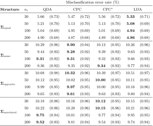
Misclassification error rates for the test samples per simulation run for thep= 2 case, together with standard errors, are reported in Table 1. For equal population covariance matrices, LDA showed the smallest misclassification error rate, followed closely by CPC and CPC?. QDA performed the worst of the four discriminant functions in this scenario.
In the CPC scenario where the common eigenvectors have the same rank order in the two population covariance matrices,CPC performed the best andLDA the worst. Only for the largest sample size (ni = 200) did CPC? slightly outperform CPC. It also seems as if QDA and CPC
perform about equally well for larger sample sizes (n1 = 100,200) in this scenario.
When the common eigenvectors have exactly the opposite rank orders in the two population covariance matrices, the CPC discriminant functions performed the best. However, the advantage of CPC and CPC? overQDAand LDA decrease as the sample size increases.
In the unrelated covariance matrices scenarios, CPC? fared the best for smaller sample sizes (ni = 30,50), but was outperformed by the theoretically correctQDAdiscriminant function for the
larger sample sizes (ni = 100,200). LDA had lower misclassification error rates than CPC in this
scenario.
However, when considering the standard errors of the misclassification error rates (given in brackets in Table 1), it is clear that the observed differences are not statistically significant in any of the scenarios for thep= 2 case.
Table 1: Simulation results for k = 2 samples of equal sizes drawn from bivariate normally dis-tributed populations. Each of the values in the table were calculated from 1,000 simulation runs. Standard errors are in brackets.
Misclassification error rate (%)
Structure ni QDA CPC CPC? LDA
Σequal 30 5.66 (0.73) 5.47 (0.72) 5.56 (0.72) 5.33 (0.71) 50 5.21 (0.70) 5.13 (0.70) 5.13 (0.70) 5.08 (0.69) 100 5.04 (0.69) 4.95 (0.69) 5.01 (0.69) 4.94 (0.69) 200 4.90 (0.68) 4.87 (0.68) 4.89 (0.68) 4.86 (0.68) Σsame 30 10.29 (0.96) 9.90 (0.94) 10.13 (0.95) 10.26 (0.96) 50 9.44 (0.92) 9.28 (0.92) 9.39 (0.92) 9.63 (0.93) 100 9.31 (0.92) 9.31 (0.92) 9.32 (0.92) 9.66 (0.93) 200 9.36 (0.92) 9.35 (0.92) 9.34 (0.92) 9.77 (0.94) Σopposite 30 10.68 (0.98) 10.32 (0.96) 10.39 (0.97) 10.51 (0.97) 50 10.12 (0.95) 10.02 (0.95) 10.00 (0.95) 10.11 (0.95) 100 9.99 (0.95) 9.97 (0.95) 10.00 (0.95) 10.16 (0.96) 200 9.65 (0.93) 9.61 (0.93) 9.63 (0.93) 9.80 (0.94) Σunrelated 30 10.18 (0.96) 10.16 (0.96) 10.12 (0.95) 10.15 (0.95) 50 10.22 (0.96) 10.28 (0.96) 10.15 (0.96) 10.21 (0.96) 100 9.75 (0.94) 10.01 (0.95) 9.77 (0.94) 9.95 (0.95) 200 9.52 (0.93) 9.81 (0.94) 9.54 (0.93) 9.74 (0.94)
4.2 The p= 5 variables case
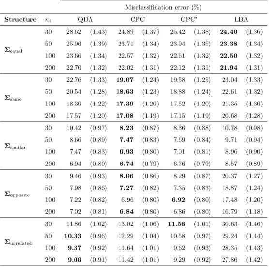
The misclassification error rates and standard errors calculated from the 30% test samples for the
p = 5 case are reported in Table 2. As expected, for equal population covariance matrices, LDA
gave the smallest misclassification error rates for all of the sample sizes. However, the differences in misclassification error rates were not statistically significant, as can be seen from the standard errors. Although the error rate differences betweenLDAand the other three discriminant functions decrease with an increase in sample size, the equal covariance matrices model is the most parsimonious (compared to the CPC and unrelated covariance matrix models) and therefore performs the best.
QDA is also theoretically correct but employs the least parsimonious of the covariance matrix models, and performed the worst for all sample sizes considered. These results concur with those reported by Flury et al. (1994) and Bianco et al. (2008).
Table 2: Simulation results for k = 2 samples of equal sizes drawn from multivariate normally distributed populations with p= 5 variables. Each of the values in the table were calculated from 1,000 simulation runs. Standard errors are in brackets.
Misclassification error (%)
Structure ni QDA CPC CPC? LDA
Σequal 30 28.62 (1.43) 24.89 (1.37) 25.42 (1.38) 24.40 (1.36) 50 25.96 (1.39) 23.71 (1.34) 23.94 (1.35) 23.38 (1.34) 100 23.66 (1.34) 22.57 (1.32) 22.61 (1.32) 22.50 (1.32) 200 22.70 (1.32) 22.02 (1.31) 22.12 (1.31) 21.94 (1.31) Σsame 30 22.76 (1.33) 19.07 (1.24) 19.58 (1.25) 23.04 (1.33) 50 20.54 (1.28) 18.63 (1.23) 18.88 (1.24) 22.61 (1.32) 100 18.30 (1.22) 17.39 (1.20) 17.52 (1.20) 21.35 (1.30) 200 17.57 (1.20) 17.08 (1.19) 17.15 (1.19) 20.68 (1.28) Σsimilar 30 10.42 (0.97) 8.23 (0.87) 8.36 (0.88) 10.78 (0.98) 50 8.66 (0.89) 7.47 (0.83) 7.69 (0.84) 9.71 (0.94) 100 7.47 (0.83) 6.93 (0.80) 7.01 (0.81) 8.96 (0.90) 200 6.94 (0.80) 6.74 (0.79) 6.76 (0.79) 8.57 (0.89) Σopposite 30 9.46 (0.93) 8.06 (0.86) 8.29 (0.87) 20.37 (1.27) 50 7.98 (0.86) 7.27 (0.82) 7.35 (0.83) 18.87 (1.24) 100 7.22 (0.82) 6.96 (0.80) 6.92 (0.80) 17.48 (1.20) 200 7.02 (0.81) 6.84 (0.80) 6.86 (0.80) 16.79 (1.18) Σunrelated 30 11.86 (1.02) 13.02 (1.06) 11.56 (1.01) 30.63 (1.46) 50 10.33 (0.96) 12.29 (1.04) 10.58 (0.97) 29.24 (1.44) 100 9.37 (0.92) 11.64 (1.01) 9.62 (0.93) 28.35 (1.43) 200 9.06 (0.91) 11.42 (1.01) 9.29 (0.92) 27.86 (1.42)
For the CPC situation when the rank orders of the common eigenvectors in the two population covariance matrices were exactly the same,CPC performed the best, followed by CPC? and QDA.
LDA performed the worst for this covariance structure. For population covariance matrices with similar rank orders of thep common eigenvectors in the population covariance matrices,CPC and
CPC? again performed the best, and LDA the worst. Again, for both Σsame and Σsimilar, the
misclassification error rates for the different discriminant functions were not significantly different. CPC discrimination seems to offer a real improvement over QDA and LDA, particularly for smaller sample sizes, in the CPC case where the common eigenvectors have opposite rank orders in the two population covariance matrices. In these scenarios CPC and CPC? performed the best, followed by the (also theoretically correct)QDAdiscriminant function. LDA gave very large misclassification error rates compared to the other three discriminant functions.
In the unrelated covariance matrices scenario, QDA fared the best, except for the smallest sample size (n1 = 30) where it was marginally outperformed byCPC?. LDAclearly performed the worst of the four discriminant functions in this scenario, giving very large misclassification error rates.
The benefit of using the more parsimonious CPC model becomes more apparent as the number of dimensions increases (Flury and Schmid, 1992). Aspand/orkincrease, the difference in number of parameters between the CPC covariance matrix estimator and the unbiased estimator increases. The value of the CPC model in the discriminant analysis context seems to be in situations where there are common eigenvectors in the population covariance matrices. In this case the CPC esti-mators will generally approximate the population covariance matrix shapes better than the pooled covariance matrix estimator, and will give more precise estimates than when using the unbiased sample covariance matrices, particularly for smaller samples.
4.3 The p= 10 variables case
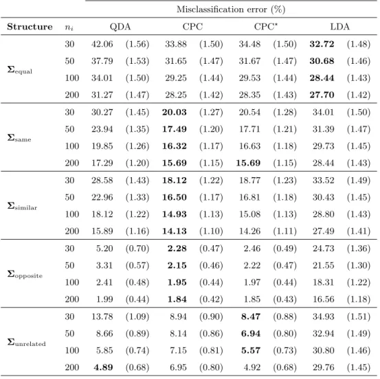
Misclassification error rates calculated from the 30% test samples per simulation run in each of the
p= 10 scenarios, together with standard errors, are reported in Table 3. As in the p = 2,5 cases,
LDAshowed the smallest misclassification error rate for equal population covariance matrices. QDA
performed significantly worse than the other discriminant functions in this scenario.
Table 3: Simulation results for k = 2 samples of equal sizes drawn from multivariate normally distributed populations withp= 10 variables. Each of the values in the table were calculated from 1,000 simulation runs. Standard errors are in brackets.
Misclassification error (%)
Structure ni QDA CPC CPC? LDA
Σequal 30 42.06 (1.56) 33.88 (1.50) 34.48 (1.50) 32.72 (1.48) 50 37.79 (1.53) 31.65 (1.47) 31.67 (1.47) 30.68 (1.46) 100 34.01 (1.50) 29.25 (1.44) 29.53 (1.44) 28.44 (1.43) 200 31.27 (1.47) 28.25 (1.42) 28.35 (1.43) 27.70 (1.42) Σsame 30 30.27 (1.45) 20.03 (1.27) 20.54 (1.28) 34.01 (1.50) 50 23.94 (1.35) 17.49 (1.20) 17.71 (1.21) 31.39 (1.47) 100 19.85 (1.26) 16.32 (1.17) 16.63 (1.18) 29.73 (1.45) 200 17.29 (1.20) 15.69 (1.15) 15.69 (1.15) 28.44 (1.43) Σsimilar 30 28.58 (1.43) 18.12 (1.22) 18.77 (1.23) 33.52 (1.49) 50 22.96 (1.33) 16.50 (1.17) 16.81 (1.18) 30.43 (1.45) 100 18.12 (1.22) 14.93 (1.13) 15.08 (1.13) 28.80 (1.43) 200 15.89 (1.16) 14.13 (1.10) 14.26 (1.11) 27.49 (1.41) Σopposite 30 5.20 (0.70) 2.28 (0.47) 2.46 (0.49) 24.73 (1.36) 50 3.31 (0.57) 2.15 (0.46) 2.22 (0.47) 21.55 (1.30) 100 2.41 (0.48) 1.95 (0.44) 1.97 (0.44) 18.31 (1.22) 200 1.99 (0.44) 1.84 (0.42) 1.85 (0.43) 16.56 (1.18) Σunrelated 30 13.78 (1.09) 8.94 (0.90) 8.47 (0.88) 34.93 (1.51) 50 8.66 (0.89) 8.14 (0.86) 6.94 (0.80) 32.94 (1.49) 100 5.85 (0.74) 7.15 (0.81) 5.57 (0.73) 30.80 (1.46) 200 4.89 (0.68) 6.95 (0.80) 4.92 (0.68) 29.76 (1.45)
CPC gave the smallest misclassification error rate, followed closely by CPC?. When the rank orders of the common eigenvectors in the population covariance matrices were similar, CPC and
CPC? again performed the best, as was also found in the p = 2 and 5 cases. With opposite rank orders of the common eigenvectors in the two population covariance matrices, theCPC andCPC?
discriminant functions clearly gave the smallest misclassification error rates. This is the situation where CPC discrimination offers the greatest advantage over QDAand LDA.
Flury et al. (1994) and Bianco et al. (2008) found CPC discrimination and QDA to perform equally well for unrelated population covariance matrices. However, in this simulation experiment for populations with p = 10 variables, CPC? fared the best in the unrelated covariance matrices scenario, except for the largest sample size considered (ni = 200) where it was outperformed slightly
by QDA. There may be two reasons for this surprising result: Firstly,CPC? employs a more par-simonious covariance matrix model than QDA. Thus, even though the CPC model is theoretically incorrect in this case, the reduction in number of parameters to estimate makes the estimation process more stable, particularly for smaller sample sizes. Secondly, by using appropriately large values for the shrinkage intensity parameter in (11), the regularised CPC estimator (used inCPC?) can model the unrelated covariance matrices as accurately as the the unbiased estimator (used in
QDA). However, as the sample sizes increase, the unbiased covariance matrix estimator becomes more accurate in estimation of the population covariance matrices.
LDA gives the largest misclassification error rate when the covariance matrices are unrelated. This concurs with the results from the simulation studies reported by Flury et al. (1994) and Bianco et al. (2008).
5
Conclusions
In this paper CPC and regularised CPC covariance matrix estimators were used to construct CPC discriminant functions. CPC discrimination was compared to ordinary quadratic discrimination (QDA) and linear discrimination (LDA) in a Monte Carlo simulation study. It was shown that CPC discrimination outperforms both QDA and LDA when two population covariance matrices are not equal or proportional, but have common eigenvectors. As expected, LDA performs the best when the population covariance matrices are equal, and QDA generally performs the best when
the covariance matrices are unrelated.
Observed misclassification error differences between the four discriminant functions were not statistically significant in most of the scenarios considered, with some important exceptions: CPC discrimination proved to perform significantly better than QDA and LDA in situations where the sample size is small relative to the number of variables and the populations have CPC covariance matrix structures. If there is uncertainty about the number of common eigenvectors in two popu-lation covariance matrices, this result implies that CPC discrimination will be a suitable choice, as it will at worst perform similar to LDA and QDA.
The rank orders of the common eigenvectors in the covariance matrices, and the locations of the different populations (i.e. the population centroids) influence the orientations and positions of the estimated covariance matrix shapes in p-dimensional space. Flury et al. (1994) and Bianco et al. (2008) hinted at the influence of these factors, but more work is needed to clarify the exact nature of their influence on the four discriminant functions presented here.
Schmid (1987) and Flury et al. (1994) have shown that discrimination under the assumption of proportional covariance matrices perform well even in situations where it is theoretically incorrect (as in the case when the covariance matrices are not proportional but have common eigenvectors). It will be interesting to compare the performance of regularised CPC discriminant analysis to discriminant analysis using the proportional covariance matrix estimators, particularly in the CPC and partial CPC contexts.
The simulation results presented in this paper are for the simplest case of two groups. CPC discriminant analysis can be extended in a straightforward way to three or more groups, by plug-ging the CPC or regularised CPC covariance matrix estimators into the appropriate discriminant functions. With an increase in the number of groups, the number of parameters to estimate for the unbiased covariance matrices model grows at a faster rate than that of the CPC model. It is thus expected that the advantage of CPC discrimination over ordinary quadratic discrimination will be more evident for a larger number of groups. However, a proper analysis of CPC discrimination in the case of three or more groups will necessitate further simulation experiments, and is a topic for future research.
Acknowledgement
The authors wish to express their thanks to the anonymous reviewer whose comments led to an improved version of this paper.
References
Bianco, A., Boente, G., Pires, A.M. and Rodrigues, I.M. (2008). Robust discrimination under a hierarchy on the scatter matrices. Journal of Multivariate Analysis,99(6): 1332–1357.
Fisher, R.A. (1938). The statistical utilization of multiple measurements. Annals of Eugenics,
8(4): 376–386.
Flury, B. (1988). Common Principal Components and Related Multivariate Models. Wiley.
Flury, B.N. and Gautschi, W. (1986). An algorithm for simultaneous orthogonal transformation of several positive definite symmetric matrices to nearly diagonal form. SIAM Journal on Scientific and Statistical Computing,7(1): 169–184.
Flury, B.W. and Schmid, M.J. (1992). Quadratic discriminant functions with constraints on the covariance matrices: Some asymptotic results. Journal of Multivariate Analysis,40(2): 244–261. Flury, B.W., Schmid, M.J. and Narayanan, A. (1994). Error rates in quadratic discrimination with constraints on the covariance matrices. Journal of Classification,11(1): 101–120.
Friedman, J.H. (1989). Regularized discriminant analysis. Journal of the American Statistical Association,84(405): 165–175.
Hastie, T., Tibshirani, R., and Friedman, J. (2009).The Elements of Statistical Learning. Springer. Johnson, R.A. and Wichern, D.W. (2002). Applied Multivariate Statistical Analysis. Prentice Hall. O’Neill, T.J. (1984). A Theoretical Method of Comparing Classification Rules under Non-optimal Conditions with Application to the Estimates of Fisher’s Linear and the Quadratic Discriminant Rules under Unequal Covariance Matrices. Technical report, Stanford University.
thesis, Department of Statistics and Actuarial Science, Stellenbosch University.
Pepler, P.T., Uys, D.W. and Nel, D.G. (2014). A comparison of some methods for the selection of a common eigenvector model for the covariance matrices of two groups. Communications in Statistics – Simulation and Computation. [In press].
Pepler, P.T., Uys, D.W. and Nel, D.G. (2015). Regularised covariance matrix estimation under the common principal components model. Communications in Statistics – Simulation and Computa-tion. [In press].
R Development Core Team (2013). R: A Language and Environment for Statistical Computing. R Foundation for Statistical Computing.
Schmid, M.J. (1987). Anwendungun der Theorie proportionaler Kovarianzmatrizen und gemein-samer Hauptkomponenten auf die quadratische Diskriminanzanalyse. PhD thesis, University of Berne.
Appendix
The covariance matrices used for the simulation study presented in this paper are given below. Fork= 2 multivariate normally distributed populations withp= 2 variables, the following four sets of population covariance matrices were used:
1) Equal covariance matrices (Σequal)
Σ1=Σ2 = 15.90 0.87 0.87 8.10
2) CPC: Same rank order of the common eigenvectors (Σsame)
Σ1= 14.20 3.34 3.34 9.80 Σ2= 22.20 3.34 3.34 17.80
3) CPC: Opposite rank orders of the common eigenvectors (Σopposite)
Σ1 = 21.12 2.68 2.68 13.88 Σ2 = 17.08 −3.27 −3.27 25.92
4) Unrelated covariance matrices (Σunrelated) Σ1 = 14.97 3.72 3.72 20.03 Σ2 = 17.17 −3.40 −3.40 25.83
Fork= 2 multivariate normally distributed populations withp= 5 variables, the following five sets of population covariance matrices were used:
1) Equal covariance matrices (Σequal)
Σ1 =Σ2= 7.00 2.14 1.43 2.63 3.31 2.14 5.91 −1.65 4.27 1.87 1.43 −1.65 4.57 −1.15 2.06 2.63 4.27 −1.15 7.14 4.21 3.31 1.87 2.06 4.21 6.38 .
2) CPC: Same rank order of the common eigenvectors (Σsame)
Σ1 = 7.00 2.14 1.43 2.63 3.31 2.14 5.91 −1.65 4.27 1.87 1.43 −1.65 4.57 −1.15 2.06 2.63 4.27 −1.15 7.14 4.21 3.31 1.87 2.06 4.21 6.38 Σ2 = 9.81 2.50 3.61 3.88 6.20 2.50 8.78 −4.08 7.50 2.35 3.61 −4.08 7.92 −2.78 4.29 3.88 7.50 −2.78 10.22 6.05 6.20 2.35 4.29 6.05 9.06 .
Σ1= 12.13 6.51 4.37 0.81 5.92 6.51 11.63 −1.42 0.62 2.57 4.37 −1.42 8.86 4.25 3.59 0.81 0.62 4.25 7.79 −1.28 5.92 2.57 3.59 −1.28 4.68 Σ2 = 8.33 5.36 3.17 0.36 4.47 5.37 13.40 −7.78 −4.39 1.54 3.17 −7.78 14.39 8.98 2.79 0.36 −4.39 8.99 9.21 −0.32 4.47 1.54 2.79 −0.32 3.17 .
4) CPC: Opposite rank orders of the common eigenvectors (Σopposite)
Σ1 = 3.07 1.88 2.89 0.41 2.43 1.88 9.71 5.45 −0.32 0.98 2.89 5.45 8.37 −0.60 1.64 0.41 −0.32 −0.60 4.16 2.66 2.43 0.98 1.64 2.66 5.69 Σ2= 11.58 −0.08 −2.89 1.51 −4.80 −0.08 2.60 −1.70 −0.12 0.13 −2.89 −1.70 4.06 0.73 0.02 1.51 −0.12 0.73 6.19 −3.73 −4.80 0.13 0.02 −3.73 6.58 .
Σ1 = 7.21 1.18 1.78 1.01 −0.65 1.18 4.27 0.70 1.24 −0.05 1.78 0.70 5.69 4.01 4.66 1.01 1.24 4.01 6.68 5.05 −0.65 −0.05 4.66 5.05 7.16 Σ2 = 5.11 2.79 6.86 −0.33 2.91 2.79 12.22 4.94 9.47 0.15 6.86 4.94 9.99 0.29 3.30 −0.33 9.47 0.29 12.79 −1.12 2.91 0.15 3.30 −1.12 5.69 .
For k= 2 multivariate normally distributed populations with p= 10 variables, the following five sets of population covariance matrices were used:
1) Equal covariance matrices (Σequal)
Σ1=Σ2= 9.75 5.35 0.07 0.55 2.54 1.07 2.94 1.07 1.93 3.77 5.35 13.04 3.60 0.26 1.38 −0.70 4.18 0.67 3.90 2.66 0.07 3.60 14.95 −0.47 1.92 −0.87 6.22 6.40 1.71 3.90 0.55 0.26 −0.47 9.80 2.87 4.27 2.22 0.85 7.04 1.19 2.54 1.38 1.92 2.87 9.69 0.68 0.78 4.28 0.33 −0.97 1.07 −0.70 −0.87 4.27 0.68 10.74 2.72 2.15 2.34 −0.92 2.94 4.18 6.22 2.22 0.78 2.72 11.58 5.28 2.09 2.74 1.07 0.67 6.40 0.85 4.28 2.15 5.28 9.92 −2.12 2.48 1.93 3.90 1.71 7.04 0.33 2.34 2.09 −2.12 11.90 1.11 3.77 2.66 3.90 1.19 −0.97 −0.92 2.74 2.48 1.11 8.64 .
Σ1= 9.75 5.35 0.07 0.55 2.54 1.07 2.94 1.07 1.93 3.77 5.35 13.04 3.60 0.26 1.38 −0.70 4.18 0.67 3.90 2.66 0.07 3.60 14.95 −0.47 1.92 −0.87 6.22 6.40 1.71 3.90 0.55 0.26 −0.47 9.80 2.87 4.27 2.22 0.85 7.04 1.19 2.54 1.38 1.92 2.87 9.69 0.68 0.78 4.28 0.33 −0.97 1.07 −0.70 −0.87 4.27 0.68 10.74 2.72 2.15 2.34 −0.92 2.94 4.18 6.22 2.22 0.78 2.72 11.58 5.28 2.09 2.74 1.07 0.67 6.40 0.85 4.28 2.15 5.28 9.92 −2.12 2.48 1.93 3.90 1.71 7.04 0.33 2.34 2.09 −2.12 11.90 1.11 3.77 2.66 3.90 1.19 −0.97 −0.92 2.74 2.48 1.11 8.64 Σ2= 12.72 11.23 −0.14 1.02 3.24 0.21 4.10 0.23 4.07 5.54 11.23 19.39 5.03 −0.34 0.61 −3.83 5.90 −1.27 7.33 6.78 −0.14 5.03 21.54 −1.95 2.58 −2.00 10.94 11.85 −0.07 6.70 1.02 −0.34 −1.95 15.25 4.51 10.17 3.77 0.92 12.78 −0.19 3.24 0.61 2.58 4.51 11.18 3.73 2.78 7.58 −0.04 −1.06 0.21 −3.83 −2.00 10.17 3.73 14.98 4.10 4.24 5.45 −2.37 4.11 5.90 10.94 3.77 2.78 4.10 13.79 9.13 3.38 4.93 0.23 −1.27 11.85 0.92 7.58 4.24 9.13 14.98 −5.05 2.85 4.07 7.33 −0.07 12.78 −0.04 5.45 3.38 −5.05 18.38 2.08 5.54 6.78 6.70 −0.19 −1.06 −2.37 4.93 2.85 2.08 8.60 .
3) CPC: Similar rank orders of the common eigenvectors (Σsimilar)
Σ1= 8.95 −1.55 1.36 2.30 5.69 3.48 4.19 2.30 4.26 1.76 −1.55 13.94 −1.02 2.27 1.26 −0.73 1.52 −0.70 0.81 4.15 1.36 −1.02 11.31 5.43 5.24 4.12 3.28 5.02 −0.50 −2.51 2.30 2.27 5.43 11.06 2.31 1.66 1.94 4.01 1.45 1.35 5.69 1.25 5.24 2.31 11.77 3.04 2.93 3.74 2.49 2.19 3.48 −0.73 4.12 1.66 3.04 10.93 0.31 3.06 7.14 0.53 4.19 1.52 3.28 1.94 2.93 0.31 10.47 0.05 1.29 −0.71 2.30 −0.70 5.02 4.01 3.74 3.06 0.05 8.09 0.24 0.91 4.26 0.81 −0.50 1.45 2.49 7.14 1.29 0.24 10.43 4.07 1.77 4.15 −2.51 1.35 2.19 0.53 −0.71 0.91 4.07 13.05
Σ2= 9.77 −5.31 −0.52 −0.99 5.81 6.14 3.97 0.98 7.92 1.82 −5.31 28.64 −0.10 9.34 2.44 −8.83 4.72 −0.35 −4.49 10.69 −0.52 −0.10 15.59 9.47 5.81 0.84 4.93 7.72 −6.45 −7.19 −0.99 9.34 9.47 14.26 3.67 −2.57 3.44 6.19 −4.42 0.99 5.81 2.44 5.81 3.67 10.44 2.07 4.62 3.92 1.57 2.12 6.14 −8.83 0.84 −2.57 2.07 15.45 −2.89 2.26 13.23 0.92 3.97 4.72 4.93 3.44 4.62 −2.89 12.35 −0.11 −1.98 −1.97 0.98 −0.35 7.72 6.19 3.92 2.26 −0.11 7.79 −2.02 −0.73 7.92 −4.49 −6.46 −4.42 1.57 13.23 −1.98 −2.02 17.54 7.99 1.82 10.69 −7.19 0.99 2.12 0.92 −1.97 −0.73 7.99 18.97 .
4) CPC: Opposite rank orders of the common eigenvectors (Σopposite)
Σ1= 12.82 2.71 1.07 0.93 4.69 3.71 0.76 1.94 4.00 0.25 2.71 12.80 1.97 4.33 6.05 3.29 −1.64 0.82 1.29 −2.78 1.07 1.97 5.18 3.41 1.69 1.84 2.60 1.16 1.06 4.24 0.93 4.33 3.41 7.42 4.03 2.34 1.88 2.71 1.56 2.51 4.69 6.05 1.68 4.03 11.40 0.68 1.50 0.64 2.72 2.56 3.71 3.29 1.84 2.34 0.68 8.58 3.19 4.57 −0.67 1.88 0.76 −1.64 2.60 1.88 1.50 3.19 11.42 7.83 −3.20 8.64 1.94 0.82 1.16 2.71 0.64 4.57 7.83 10.03 −2.66 2.81 4.00 1.29 1.06 1.56 2.72 −0.67 −3.20 −2.66 12.86 0.79 0.25 −2.78 4.24 2.51 2.56 1.88 8.64 2.81 0.79 16.49 Σ2= 6.32 0.96 −1.44 2.37 −3.34 −3.17 0.07 −1.07 −1.95 1.09 0.96 8.11 −2.50 −1.56 −4.42 −3.28 1.71 −0.32 0.28 2.36 −1.44 −2.50 17.33 −6.64 2.61 −0.28 −2.16 2.41 −0.28 −3.68 2.37 −1.56 −6.64 13.40 −3.50 −1.20 1.53 −3.82 −1.41 −0.10 −3.34 −4.42 2.61 −3.50 9.13 3.14 −2.02 1.36 −0.15 −1.98 −3.17 −3.28 −0.28 −1.20 3.14 10.33 0.31 −3.36 0.84 −1.69 0.07 1.71 −2.16 1.53 −2.02 0.31 17.27 −11.01 2.59 −6.53 −1.07 −0.32 2.41 −3.82 1.36 −3.36 −11.01 14.26 0.20 3.17 −1.95 0.28 −0.28 −1.41 −0.15 0.84 2.59 0.20 5.37 −1.38 1.09 2.36 −3.68 −0.10 −1.98 −1.69 −6.53 3.17 −1.38 7.47 .
5) Unrelated covariance matrices (Σunrelated) Σ1= 6.19 2.35 −0.76 2.34 3.18 2.97 1.81 1.20 2.73 −0.82 2.35 6.21 0.48 2.32 1.51 1.38 3.95 −0.46 4.31 0.82 −0.76 0.48 5.98 −0.10 −0.34 0.23 2.20 2.56 −1.39 1.00 2.34 2.32 −0.10 3.75 0.03 0.60 0.75 0.21 1.62 1.40 3.18 1.51 −0.34 0.03 6.89 3.69 1.07 1.55 4.17 −0.15 2.97 1.38 0.23 0.60 3.69 6.14 0.49 3.49 1.76 −0.02 1.81 3.95 2.20 0.75 1.07 0.49 10.65 −3.07 1.36 0.14 1.20 −0.46 2.56 0.21 1.55 3.49 −3.07 9.59 −1.02 0.59 2.73 4.31 −1.39 1.62 4.17 1.76 1.36 −1.02 8.79 1.07 −0.82 0.82 1.00 1.40 −0.15 −0.02 0.14 0.59 1.07 5.62 Σ2= 10.89 5.23 7.56 11.23 −2.78 2.50 −1.29 2.14 0.19 0.84 5.23 12.66 1.12 9.43 0.20 0.85 5.51 2.39 −0.23 2.38 7.56 1.12 22.15 6.96 −5.91 7.38 0.79 7.60 5.92 2.52 11.23 9.43 6.96 22.06 5.87 7.04 2.96 −0.82 −1.19 7.93 −2.78 0.20 −5.91 5.87 41.71 6.03 10.24 0.72 5.89 22.49 2.50 0.85 7.38 7.04 6.03 9.52 3.53 −0.29 4.18 6.27 −1.29 5.51 0.79 2.96 10.24 3.53 14.46 4.70 5.90 11.44 2.14 2.39 7.60 −0.82 0.72 −0.29 4.70 14.89 5.40 7.47 0.19 −0.23 5.92 −1.19 5.89 4.18 5.90 5.40 11.78 5.62 0.84 2.38 2.52 7.93 22.49 6.27 11.44 7.47 5.62 21.48 .