Chapter 5 Adaptive Mesh, Embedded Boundary Model for Flood Modeling

(1)

Methodology for Flow and Salinity Estimates in the

Sacramento-San Joaquin Delta and Suisun Marsh

32nd Annual Progress Report

June 2011

Chapter 5

Adaptive Mesh, Embedded Boundary Model for

Flood Modeling

Authors: Qiang Shu and Eli Ateljevich,

Delta Modeling Section,

Bay-Delta Office,

(2)

Methodology for Flow and Salinity Estimates 32ndAnnual Progress Report

(3)

Page 5-iii Adaptive Mesh, Embedded Boundary Model for Flood Modeling

Dam Break on a Wet Bottom ... 5-9

5.6.3

Dam Break on a Dry Bottom with Friction ... 5-10

5.7

Applications and Challenges ... 5-10

5.8

Acknowledgements ... 5-11

5.9

References ... 5-11

Figures

Figure 5-1 A multiblock adaptive mesh hierarchy with a refinement factor of 2 between levels ... 5-4 Figure 5-2 Decomposition of a patch of cells into regular, irregular, and covered cells ... 5-5 Figure 5-3 Two depictions of flooding ... 5-6 Figure 5-4 AMR resolving a flood along a reach of the Sacramento River ... 5-7 Figure 5-5 Water depth (left) and velocity (right) after dam break at time 50.78 seconds ... 5-8 Figure 5-6 Water depth (left) and velocity (right) after dam break at time 50.52 seconds ... 5-9 Figure 5-7 Water depth (left) and velocity (right) after dam break at time 50.88 seconds ... 5-10

(4)

(5)

Page 5-1 Adaptive Mesh, Embedded Boundary Model for Flood Modeling

5

Adaptive Mesh, Embedded Boundary Model for Flood Modeling

5.1

Summary

We describe a 2-dimensional shallow water model designed to simulate water quality and flooding. The model uses a finite-volume discretization of the shallow water equations on an adaptive Cartesian mesh, using embedded boundaries to represent complex topography. For flooding applications, we use

adaptive mesh refinement (AMR) to evolve Cartesian sub-grids near a flood front, which leads to a resolved local result. Fluxes on the front itself are described using wet-dry Riemann solutions. The algorithms are implemented in parallel and highly scalable. The model is tested using analytical solutions of flood propagation on wet and dry channels and of a dam-break problem. Applications to flooding in arbitrary bathymetry are discussed.

5.2

Introduction

The California Department of Water Resources (DWR) and Lawrence Berkeley National Laboratory (LBNL) are collaboratively developing a multi-dimensional computer model to solve the shallow-water equations. The motivation of the project is to provide a high performance, accurate, and open-source tool for decision making support in the San Francisco Bay and Sacramento-San Joaquin Delta. The Bay-Delta system is a nexus of water policy debate and scientific scrutiny, with constantly shifting concerns including salt intrusion, fish and pollutant transport, water supply reliability, and flooding of Delta islands. In particular, the property and infrastructure risk posed by flood events underscores the need for models in flood risk assessment and planning.

Our shallow water model REALM (River, Estuary, and Land Model) includes a shock-capturing algorithm and 2 technologies relevant to flood modeling: adaptive mesh refinement and embedded boundaries. We employ adaptive mesh refinement (AMR) [(Berger and Oliger 1984) (Berger and Colella 1989)] to refine fronts, maintain resolution at local length scales and concentrate computational resources on predefined areas of interest. We use a Cartesian mesh with embedded boundaries (EB) to represent the natural shoreline. Although adaptive mesh refinement has been used before in flood modeling [e.g. (George 2006); (Begnudelli, Sanders and Bradford 2008)], we believe that the use of AMR and EB together is novel, particularly in context of a scalable, parallel computer architecture.

This chapter summarizes our algorithm, describes details relevant to flood modeling, and describes the verification of our model for transient flooding events using problems from the literature on wet and dry beds. We discuss wet bed applications in a natural setting with arbitrary topography, as well as some of the challenges and ambiguities of the EB-AMR approach on 2 different types of wetting and drying problems.

5.3

Governing Equations

Our shallow water model REALM is based on the 2D depth-integrated Navier-Stokes equations, with a hydrostatic treatment of pressure, Boussinesq assumption concerning salt-induced horizontal

(baroclinic) density variation and friction. The shallow water equations are commonly and efficiently used as models of flood propagation and inundation, a practice that is noted and critiqued in (Alcrudo 2002).

(6)

In terms of the height of the water column

h

, local velocities u and v and salt concentration s, the shallow water equations in conservation form are

S

y

F

x

F

t

U

x y

=

)

(

)

(

∂

+

∂

+

∂

_{Eq. 5-1}

where the conserved variable vector

T

hs

hv

hu

h

U

=

(

,

)

_{and the flux across cell faces in x and y} directions are

⎟

⎠

⎞

⎜

⎝

⎛

+

hus

huv

h

g

hu

F

x 0 2 2

2

=

ρ

Eq. 5-2

⎟

⎠

⎞

⎜

⎝

⎛

+

hvs

h

g

hv

huv

hv

F

y 0 2 2

2

=

ρ

Eq. 5-3

In these equations,

g

denotes the gravitational constant,

ρ

0_{denotes the density of fresh water, and}

) ( =

ρ

s

ρ

_{is an equation of state. To focus on flooding and the hyperbolic component of our solver,}

(7)

The sources and sinks include pressure forces from the bed, friction stress, and other local sources of mass or momentum such as wind or Coriolis acceleration. Here we consider only bottom pressure and friction: T y y x x hb g hb g S _⎥ ⎦ ⎤ ⎢ ⎣ ⎡ − − − − , ,0 , 0 = 0 0

τ

ρ

τ

ρ

_{Eq. 5-4}

where

b

x_andby_{are the slope of the bed in x and y direction and}

τ

x_{is a bottom stress given by the} Chezy formula (Molls, Zhao and Molls 1998):

2 2 2 0 = u u v C x +

ρ

τ

Eq. 5-5 2 2 2 0 = v u v C y +

ρ

τ

Eq. 5-6

where

C

is the Chezy coefficient.

5.4

Solution Algorithm

We use a finite volume discretization of the shallow water equations, based on a Cartesian grid with embedded boundaries representing shorelines. Data are collocated at cell centers. Our algorithm is best articulated in 3 tiers:

AMR: Adaptive mesh refinement orchestrates integration over the multiple levels of grids refined in space and time.

EB: We use a special treatment on the cell containing shoreline.

Godunov: Single grid computations are handled by a second order Godunov scheme with corner transport upwind (CTU) treatment of fluxes at cell faces.

(8)

Methodolo Page 5-4 5.4.1 A In the org sequentia algorithm al. (1995) AMR hiera coarse int completio underlyin result is a criteria fo extrapola N fo Fi of

ogy for Flow an

Adaptive Me ganization of o ally advancing m follows Berg for embedde archy are inte terfaces (dots on of the time g coarse cells conservative or refining cel tion) error es

ote: Coarse cells or the fine mesh

igure 5-1 A mu f 2 between le

nd Salinity Esti

esh Refinem our algorithm g the time ste ger and Colell ed boundarie egrated from s) are used to e step, fine ce s. When regri e, consistent e ls, including u stimates, pres s adjacent to fin ultiblock adapt evels mates A ment m, adaptive m ep at different a (1989) as m s. The cycle o coarse to fin o help estimat ell states and dding occurs, estimate ove user-prescribe sence of a we

e cells (dots) are

tive mesh hier

daptive Mesh, mesh refineme t levels of ref modified by Co of information e. Between le te boundary c fine cell fluxe , further inter r the hierarch ed refinemen et-dry interfac e used to provid archy with a re , Embedded Bo

ent plays the finement. The olella, Graves n is depicted evels, results conditions fo es are averag rpolation is re hy. Our AMR nt, refinemen ce, or sharp g de boundary con efinement fac 32ndAnn oundary Mode role of an out e AMR compo s, et al. (2006 in Figure 5-1. in coarse cel r the next fin ed and used equired to fill approach allo t based on (R gradients. nditions tor nual Progress R l for Flood Mo ter controller onent of our ) and Pember . Levels of the ls abutting fin er level. Upo to replace da l new levels. T ows flexible Richardson Report odeling r, r, et e ne-n ata in The

(9)

Methodolo Page 5-5 5.4.2 E We use Ca without a 5-2 shows and cover Regular ce treated us full cell es conservat momentu momentu cells. Furt No ill Fi 5.4.3 G Within on finite volu cell faces 1. Calcu 2. Extra half t 3. Solut varia linea dens 4. Mod Corn The algor second or

ogy for Flow an

Embedded b artesian cut c steep time s s a grid inters red cells (cove

ells are integr sing a hybrid stimate, using tive divergenc um, induces th um discrepanc ther details ar

ote: Gray region ustration on the

igure 5-2 Deco

Godunov alg ne multiblock ume predicto

and then upd ulation of spa apolation in o time. tion of a Riem ables on each arized problem sity variation. dification of th ner Transport ithm produce rder accurate nd Salinity Esti boundaries cells (Colella, tep penalty in secting the bo

ered cells are rated using m update that c g weights pro ce contribute he boundary cy, and the m re discussed i ns are outside th e right side. omposition of a gorithm grid, we emp r-corrector m date cell aver atial gradients one space dim mann problem side of a face m as describe he dual, one d Upwind met e upwinded fl in smooth flo mates A Graves, et al. n partial cells oundary at a s e implied by e methods for a combines a c oportional to t es stability; th condition, an mismatch is m in Colella, Gra he domain. Cove a patch of cells

ploy the solut method: We c rage values. T s using limite mension and t ms for upwind e into upwind ed in Toro (20 dimension es hod of Colella luxes and prim ow, and robu

daptive Mesh, . 2006) to rep s due to the u shoreline. The elimination). square Carte onservative s the fraction o he conservativ nd is accurate itigated by re aves, et al. (2

ered cells have b

s into regular, tion algorithm onstruct accu The technique rs to avoid os time of variab ding, which co ded fluxes. W 006). The solu timate with f a (1990). mitive variabl ust to flow ob , Embedded Bo present natur use of an expl e grid is deco esian mesh. Ir small cell esti of the irregula

ve divergence e. The combin edistribution

006).

een removed fro

irregular, and

m in Colella, G urate, upwind e has the follo scillations nea bles from cell onvert the du We use a primi ution is modif fluxes in the t le estimates t lique to the c 32ndAnn oundary Mode ral boundaries icit integratio omposed into rregular volum mate with a n ar cell that is e preserves m nation induce of the discrep om the d covered cells Graves, et al. ( ded estimates owing attribu ar discontinu centers to ed ual estimates itive solver ba fied to include transverse dir

that are shoc coordinate fa

nual Progress R

l for Flood Mo

s with high fid on method. Fi

regular, irreg

mes of fluid a non-conserva wet. The non mass and s a mass and pancy to near (2006), which s of the fluxes tes: ities. dge centers a of extrapolat ased on the e salinity-indu rection, as in k-capturing, ces. In cells th Report odeling delity igure gular, are ative n-rby h is a s on at the ted uced the hat

(10)

intersect the shore, the upwinded primitive variables are further interpolated and combined into a conservative divergence as described in the previous section.

Source terms are integrated using Heun's method. A well known difficulty with explicit finite volume representations is maintaining quiescent flow. The pressure component of the flux must be discretized in such a way to balance the bed pressure source in quiescent flow. Otherwise, the discretization can excite flow from a fluid at rest. Our characterization of bed pressure is based on this balance using a source discetization with face contributions analogous to the face contributions to the flux divergence under the conditions that the water surface is level (at the cell center level) and velocity is zero. Because the flux divergence is a hybrid, the bed source is too. The approximation is consistent with the source terms g hb_x 0

ρ

− and g hb_y 0

ρ

− in the original partial differential equation (PDE) and preserves quiescent flow well.

5.5

Wet/Dry Front Capture

In flood modeling, one of 2 treatments of an evolving flood front is usually adopted. The first, which is common for modeling tsunamis and intertidal mudflats, is to treat front propagation as a side effect of rising or falling water on bathymetry (Figure 5-3a). The second propagates the flood as a discontinuity (Figure 5-3b) and requires the ability to track or capture the evolving front.

The results we present here are for evolution over a flood plain. We use our hyperbolic algorithm, wet-dry Riemann solvers, and AMR to capture flood waves (Figure 5-3b). We use embedded boundaries to model shores that do not move. The capability to model the interaction between water levels and bathymetry (Figure 5-3a) is a work in progress.

(11)

Methodolo Page 5-7 Fi Adaptive spawned solution. W the (in thi Due to th is inheren algorithm and appro with both As will be physics of

5.6

Mo We have a Action on descriptio tests 3, 4

ogy for Flow an

igure 5-4 AMR mesh refinem around a floo We also use d is case, static e Godunov fi ntly able to ca m, we estimate oximate state h sides dry, de seen in the n f an advancin odel Verifica applied our c Dam Break M on of the test and 5. nd Salinity Esti R resolving a flo ment is used t od wave front dry-wet interf ) levee bound nite volume d apture discon e the state on e wet/wet Rie epth and velo next section, t g flood on bo ation ode to severa Modeling) to suite is availa mates A ood along a re to help resolv t on a reach o faces as a crit daries. discretization tinuities such n the faces an emann solutio ocity are of co the model is oth wet and d

al flood and d verify the sta able in Gouta

daptive Mesh,

ach of the Sac

ve the flood w of the Sacram terion for re-g

n, upwinding, h as flood wav nd switch bet on based on w ourse always s capable of re dry beds. dam-break te ability and acc al and Maurel , Embedded Bo cramento Rive wave front. Fi mento River ba gridding. Emb and use of gr ves and wet-d ween an exac whether the f set to zero. esolving and r st cases prop curacy flood a (1997). Here 32ndAnn oundary Mode r gure 5-4 show ased on the g bedded boun radient limite dry fronts. In ct wet/dry Rie faces are wet

reproducing t posed by CADA algorithms. A e we present nual Progress R l for Flood Mo ws subgrids gradient of th daries repres

ers, our algori the Godunov emann soluti or dry. On fa he shallow w AM (Concerte A detailed results for CA Report odeling e sent ithm v on aces water ed ADAM

(12)

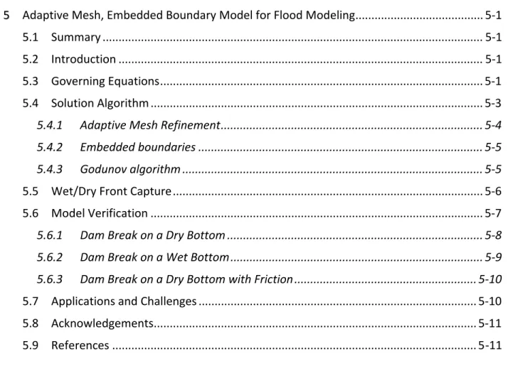
5.6.1 Dam Break on a Dry Bottom

This test problem has data containing a dry bed to the right of dam in a rectangular channel with a flat bottom. An instantaneous dam break is assumed, and unsteady flow velocity and water depth are computed by the model. An analytical solution (Ritter Solution) exists for the test and is given in Goutal and Maurel (1997). The objective of this test is to test the stability of the code in simulating the

propagation of a wave over the dry zone.

The spatial domain is represented by a 2048x16 m rectangular cross section channel, which is

discretized using 1 m square cells. The channel bottom is assumed frictionless and initial condition is set to:

⎩

⎨

⎧

0

>

if

0

=

,

0

=

0

<

if

0

=

,

6

=

x

u

m

h

x

u

m

h

The dam break occurs at x=0. The time step is adapted to maintain a Courant number of 0.9. Results for this test are shown at time=50.78s in Figure 5-5.

The simulated dry/wet surface matches the analytical solution well. In Figure 5-5 REALM correctly simulates the jump of velocity at the front without obvious oscillation.

(13)

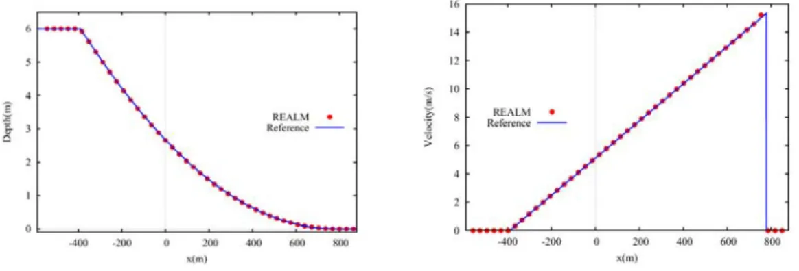
5.6.2 Dam Break on a Wet Bottom

This test problem has data containing a wet bed to the right of dam in a rectangular channel with a flat bottom. An instantaneous dam break is assumed, and unsteady flow velocity and water depth are computed by the model. An analytical solution (Goutal and Maurel 1997) exists for the test. The objective of this test is to observe the ability of the code to resolve (a) the speed of wave propagation, (b) the strength of the jump on the shock front, (c) the width of the shock layer and (d) stability in the vicinity of the shock.

The spatial domain is again represented by a 2048x16 m rectangular cross section channel discretized using 1 m size square cells. The channel bottom is assumed frictionless and initial condition is set to:

⎩

⎨

⎧

0

>

if

0

=

,

2

=

0

<

if

0

=

,

6

=

x

u

m

h

x

u

m

h

The dam is at x=0. The time step is adaptive to maintain a Courant number of 0.9. Results for this test are shown at time 50.52 seconds in Figure 5-6.

Figure 5-6 Water depth (left) and velocity (right) after dam break at time 50.52 seconds

Again REALM performs well with respect to the objectives of this test. The simulated left transonic rarefaction wave and right shock wave match their analytical counterparts as shown in Figure 5-6. The downstream wave moves faster than upstream wave, a feature of the analytical solution. In the left rarefaction wave, simulated water depth and velocity are smooth without any distinct break point. In the middle shock layer zone, both the computed water depth and velocity match the analytical solution well. There are no oscillations in the vicinity of the computed shock.

(14)

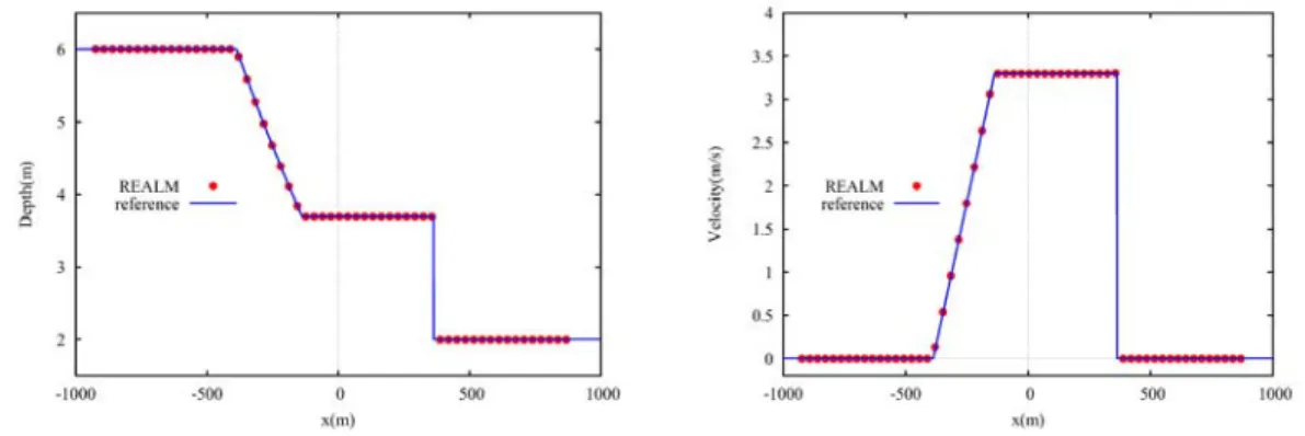
5.6.3 Dam Break on a Dry Bottom with Friction

In this test, REALM is applied to the unsteady flow resulting from an instantaneous dam breaking in a rectangular channel with constant width and with friction. Only the approximate Dressler solution (Dressler 1952) is available, the validity of which is limited to a region comprising less than one-third the distance to the point where the solution gives a zero value of flow. The objectives of this test are to validate the ability of the code to propagate a wave front over a dry bed with friction.

The spatial domain is again represented by a 2048x16 m rectangular cross section channel discretized using 1 m size square cells. The Chezy coefficient is set to 40 and the initial condition is set to:

⎩

⎨

⎧

0

>

if

0

=

,

0

=

0

<

if

0

=

,

6

=

x

u

m

h

x

u

m

h

The dam is at x=0. The time step is adaptive to maintain a Courant number of 0.9. Results for this test are shown at time 50.88 seconds in Figure 5-7.

Figure 5-7 Water depth (left) and velocity (right) after dam break at time 50.88 seconds

The simulated result shows an apparent slowing down of the wave front. This effect is caused by the friction term. Upstream of the dam, REALM correctly computes water depth and velocity. The behavior of REALM is stable in the vicinity of the wave front.

5.7

Applications and Challenges

REALM appears to do well on a class of flood evolution problems involving flat bathymetry regardless of whether the bed is wet or dry. Anecdotally, we have observed that the model also handles practical flooding problems in fully wetted channels robustly. We point out, however, that the benchmarks presented in this paper focus on flat beds. This class of problem poses some of the greatest numerical challenges for flooding, but application of REALM on wetting and drying problems dominated by topography is still under development.

One problem during drying is caused by inaccurate reconstruction of volumes, depths, and face apertures in partially wet cells from the water surface. As a cell dries, its 2D area shrinks. The

relationship between average depth and surface becomes more difficult to estimate. The cell can dry out early, and inconsistencies can develop between whether the cell is considered wet and whether a face is considered wet.

(15)

Begnudelli, Sanders, and Bradford (2008) noted similar problems and reconstruct the depth of partially dry faces by extrapolating a surface from the wet neighbors. Casulli (1990) proposes the use of a subgrid bathymetry model comprised of piecewise flat elements.

We are working to address the problem by updating the embedded boundary depiction of the domain along with fluctuations in the surface. On a domain with a steep bed, the treatment amounts to a subgrid bathymetry model. On a domain with a shallow bed slope, the flood front can move across the cell easily as a wave and be captured by the numerics, as was the case in the results presented here. Another issue we have experienced is that high fluxes tend to overdraw the adjacent cells of mass and momentum. Sleigh et al. (1998) used a limited flux to solve this issue, in which momentum flux is set to zero and only mass flux is considered. Another solution in keeping with the mechanics of our algorithm is to include the overdraft as part of mass and momentum redistribution in the EB component

algorithm, donating it to neighboring cells in proportion to the mass already contained in the cells. We also continue to hone our Riemann solutions for this application, as our approximate state Riemann solver is sometimes the source of unrealistic fluxes in extremely shallow flows.

5.8

Acknowledgements

Phillip Colella and Peter O. Schwartz of Lawrence Berkeley National Laboratory assisted with this investigation.

5.9

References

Alcrudo, F. "A state of the art review on mathematical modelling of flood propagation." 1st IMPACT Project Workshop. 2002.

Begnudelli, L., B. F. Sanders, and S. F. Bradford. "Adaptive godunov based model for flood simulation." J. Hydraul. Eng. 34(6) (2008): 714–725.

Berger, M., and J. Oliger. "Adaptive mesh refinement for hyperbolic partial differential equations." J. Comput. Phys. 53 (1984): 484–512.

Berger, M., and P. Colella. "Local adaptive mesh refinement for shock hydrodynamics." J. Comput. Phys. 82(1) (1989): 64-68.

Casulli, V. "A high-resolution wetting and drying algorithm for free-surface hydrodynamics." Int. J. Numer. Meth. Fluids 60 (1990): 391–408.

Colella, P. "Multidimensional upwind methods for hyperbolic conservation laws." J. Comput. Phys. 87 (1990): 171–200.

Colella, P., D. T. Graves, B. J. Keen, and D. Modiano. "A cartesian grid embedded boundary method for hyperbolic conservation laws." J. Comput. Phys., 2006: 347–366.

Dressler, R. F. "Hydraulic resistance effect upon the dam-break functions." J. Res. Natl. Bur. Stand. 49(3) (1952): 217–225.

George, D. "Finite volume methods and adaptive refinement for tsunami propagation and inundation." PhD thesis, University of Washington, 2006.

Ghidaglia, J. M., and F. Pascal. "On boundary conditions for multidimensional hyperbolic systems of conservation laws in the finite volume framework." CMLA, ENS de Cachan. 2002.

(16)

Goutal, N., and F. Maurel. "Description of the test cases." Proceedings of the 2nd Workshop on Dam-Break Wave Simulation. 1997. 18–28.

Molls, T., G. Zhao, and F. Molls. "Friction slope in depth-averaged flow." J. Hydraul. Eng. 124(1) (1998): 81-85.

Pember, R. B., J. B. Bell, P. Colella, and W. Y. Crutchfield. "An adaptive Cartesian grid method for unsteady compressible flow in irregular regions." J. Comput. Phys. 120(2) (1995): 278–304.

Sleigh, P. A., M. Berzins, P. H. Gaskell, and N. G. Wright. "An unstructured finite-volume algorithm for predicting flow in rivers and estuaries." Computers & Fluids 27(4) (1998): 479–508.

Toro, E. F. Shock-Capturing Methods for Free-Surface Shallow Flows. Chichester: John Wiley and Sons, 2006.

Chapter 5 Adaptive Mesh, Embedded Boundary Model for Flood Modeling

Methodology for Flow and Salinity Estimates in the

Contents

Dam Break on a Wet Bottom ... 5-9

Adaptive Mesh, Embedded Boundary Model for Flood Modeling

igure 5-1 A mu f 2 between le

igure 5-2 Deco

irregular, and

ach of the Sac

5.6.1 Dam Break on a Dry Bottom

0

0

0

0

0

5.6.2 Dam Break on a Wet Bottom

0

0

0

0

Figure 5-6 Water depth (left) and velocity (right) after dam break at time 50.52 seconds

0

0

0

0

0

Figure 5-7 Water depth (left) and velocity (right) after dam break at time 50.88 seconds