Delft Center for Systems and Control
Technical report 10-040
Demand response with micro-CHP
systems
∗
M. Houwing, R.R. Negenborn, and B. De Schutter
If you want to cite this report, please use the following reference instead:
M. Houwing, R.R. Negenborn, and B. De Schutter, “Demand response with
micro-CHP systems,”
Proceedings of the IEEE
, vol. 99, no. 1, pp. 200–213, Jan. 2011.
Delft Center for Systems and Control Delft University of Technology Mekelweg 2, 2628 CD Delft The Netherlands
phone: +31-15-278.51.19 (secretary) fax: +31-15-278.66.79
URL:http://www.dcsc.tudelft.nl
Demand Response with Micro-CHP Systems
Michiel Houwing, Rudy R. Negenborn, and Bart De Schutter
Member, IEEE
Abstract—With the increasing application of distributed energy resources and novel information technologies in the electricity infrastructure, innovative possibilities to incorporate the demand side more actively in power system operation are enabled. A promising, controllable, residential distributed generation tech-nology is a micro combined heat and power system (micro-CHP). Micro-CHP is an energy efficient technology that simultaneously provides heat and electricity to households. In this paper we investigate to what extent domestic energy costs could be reduced with intelligent, price-based control concepts (demand response). Hereby, first the performance of a standard, so-called heat-led micro-CHP system is analyzed. Then, a model predictive control strategy aimed at demand response is proposed for more intelli-gent control of micro-CHP systems. Simulation studies illustrate the added value of the proposed intelligent control approach over the standard approach in terms of reduced variable energy costs. Demand response with micro-CHP lowers variable costs for households by about 1–14 %. The cost reductions are highest with the most strongly fluctuating real-time pricing scheme.
Index Terms—micro combined heat and power systems, de-mand response, model predictive control.
I. INTRODUCTION A. Distributed generation
P
OWER generation is responsible for a large share of the anthropogenic CO2emissions [1]. Many new sustainabletechnologies for electricity provision are therefore currently under development [2]. Many of these technologies are de-signed for application at the distribution level of the electricity infrastructure. Such small-scale electricity generation systems are referred to as distributed generation (DG). Examples of DG technologies are photovoltaic systems, wind turbines, and combined heat and power plants (CHP). The use of DG has several advantages. When DG systems use renewable primary energy as input, they can provide significant environmental benefits. Due to reduced losses from electricity transport and due to cogeneration options, DG can also lead to increases in energy efficiency. Moreover, besides their environmental ben-efits, DG systems can reduce investment risks, they stimulate fuel diversification and energy autonomy, and the presence of generation close to demand can increase the power quality and reliability of delivered electricity [3]–[5]. Currently, the penetration of DG at medium and low voltages, both in distribution networks and inside customers’ households, is increasing in developed countries worldwide [3]–[7].
M. Houwing is with Eneco in the Netherlands. E-mail:
R.R. Negenborn and B. De Schutter are with the Delft Center for Sys-tems and Control, Delft University of Technology, the Netherlands. E-mail: {r.r.negenborn,b.deschutter}@tudelft.nl.
B. Micro combined heat and power systems as novel heating technology
The domestic sector is responsible for a large share of a country’s energy consumption and carbon emissions. In the Netherlands, for example, in 2007 the domestic sector represented a share of 24 % in the total electricity consumption and 20 % in the gas consumption [8], [9]. Further, Dutch households are responsible for about 18 % of the total CO2
emissions (excluding transport) in the Netherlands [8], [9]. One of the options for households to reduce electricity consumption from the grid is the installation of DG. Be-sides small wind turbines and photovoltaic systems, specific potential for applying DG at the residential level lies in utilizing electricity and heat from so-called micro combined heat and power systems (micro-CHP), also known as micro cogeneration systems. Based on [10] a micro-CHP system is defined as follows:
Micro-CHP: energy conversion unit with an electric capacity below 15 kW that simultaneously generates heat and power.
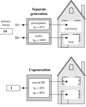
Micro-CHP systems can be relatively small and are expected to be of the same size as current heating systems. Compared to current heating systems micro-CHP is a step forward in terms of energy efficiency [10]. By generating electricity locally and utilizing the co-produced heat, the efficiency of domestic energy use is substantially improved. In Figure 1 the basic principle of micro-CHP is shown. Assuming that a household needs 20 units of electrical energy and 80 units of heat, and assuming a boiler efficiency of 100 % (based on the lower heating value of the primary fuel) and an efficiency of large power generation of 45 %, a household consumes 124 units of primary energy in the case of separate heat and power generation. With a micro-CHP system of 20 % electric and 80 % thermal efficiency, 100 units of primary energy are required, leading to primary energy savings of around 20 %.
During the last years there has been significant progress toward developing kW-scale CHP applications. Micro-CHP systems are on the verge of becoming mass marketed as a next generation domestic heating system [10], [11]. Several manufacturers are preparing market introduction and retail companies have started selling micro-CHP systems [12], [13]. The likely primary fuel for these systems is natural gas. Hence, micro-CHP is envisaged as a promising next generation heat-ing system for countries and regions with extensive natural gas infrastructures. Potential markets for micro-CHP are European countries such as the Netherlands, Germany, and Italy, as well as Japan and parts of the United States and Canada [10], [14]– [16]. In those areas, space heating and domestic hot water are mainly produced inside the house via the conversion of natural gas in boilers. District heating networks, heat pumps, and solar
electricity 80 heat 80 124 energy primary 100 80 44 Cogeneration generation Separate power plants = 45% boiler th= 100% micro−CHP 20% = th= 80% 20 20 η η η e e η
Fig. 1. Energy efficiency with micro-CHP.
boilers are only marginally used there.
C. Objective of the paper
Compared to wind turbines and photovoltaic systems, micro-CHP is a special type of DG technology in the sense that the power output can be easily controlled. This characteristic, together with the fact that micro-CHP units are mostly coupled to heat storage systems [17], creates flexibility in power gen-eration. This paper analyzes the potential value of flexibility in micro-CHP operation.
Besides the standard control strategies envisaged for micro-CHP, which are aimed at following either heat or electricity demand, there are many other control objectives for which micro-CHP systems can be deployed. Examples from [18]– [20] are the provision of intra-day balancing services, the provision of black start services and improving power quality. Another objective for which to control micro-CHP is demand response, which is the ability of domestic net-consumption of electricity to respond to real-time prices (net-consumption = consumption - production). This paper investigates the extent to which demand response with micro-CHP leads to reduced energy costs for households when compared to standard heat-led control.
D. Outline
This paper is organized as follows. In Section II we present a model of a standard heat-led control strategy and analyze the associated economic performance of the micro-CHP system for households. In Section III we then propose a more intelli-gent control strategy using so-called model predictive control to implement demand response. Via extensive simulations a comparison between the performance of this control strategy and the heat-led control system is made. This indicates the
added value for investors of intelligently using the control capabilities of micro-CHP units for the objective of demand response. Conclusions and directions for further research are given in Section IV.
II. ECONOMIC PERFORMANCE OF MICRO-CHPUNDER HEAT-LED CONTROL
In order to analyze economic savings with intelligent micro-CHP control, it is important to have a reference case, both in terms of control strategy as well as economic feasibility of the application of micro-CHP. This section describes such a reference case, where micro-CHP units are controlled in a heat-led way. Heat-led control means that the control is fo-cused on following domestic heat demand. This type of control is envisaged as the most likely standard control strategy for micro-CHP [10]. In the heat-led case micro-CHPs are placed in houses, they operate under heat-led control, and electricity is traded both ways between the retailer and households.
A. Literature on standard control of micro-CHP
There is a substantial body of literature on standard control strategies for micro-CHP systems and the associated perfor-mance. A good overview of the literature on control strategy design and cost performance is presented in [21]. In [21] it is noted that there is a multitude of possible operating strategies that can be generally classified as heat-led or electricity-led. It is concluded that the control strategy for the first generations of micro-CHPs will be heat-led or electricity-led and that future generations may incorporate cost and/or emission minimizing control.
More work on the design of standard control strategies and on the impact of control strategies on variable costs for households can be found in [15], [22]–[25]. These sources report annual energy cost savings, relative to conventional households, in the range of 8–40 %. Savings depend on the adopted control strategy, domestic energy demand and pricing regime. Throughout this paper we refer to ‘conventional house-holds’ as being households that take all electricity demand from the grid (i.e., sold to households by retailers) and that fulfill their heat demand with a conventional, gas-fired boiler. Looking at the existing literature in relation to the work presented in this section of this paper, we make the following contributions:
• Even though much work has been done on standard
control, a reference will need to be developed here to serve as a basis against which more intelligent control schemes can be compared. The existing literature helps in making the modeling choices and assumptions for the model of heat-led control developed here and forms a validation for the simulation results. Further, the heat-led control strategy that is developed in Section II-B2, aimed at having as few prime mover start-ups as possible, is a novel strategy and is not described in the literature. Many start-ups are unwanted, as these create mechanical wear and additional gas use for fuel cells (this is explained in Section II-B1).
• The economic analyses in the literature consider only
fixed tariffs for imported and fed-back electricity. As there are also time-varying tariffs possible for households and as these tariffs might influence the economic per-formance of micro-CHP, the literature is limited in this respect. Here, we also look at time-varying tariffs.
B. Modeling heat-led control of micro-CHP
This section presents mathematical models of the system under study and of the standard heat-led control strategy for the micro-CHP systems.
1) System description: The household-retailer system under consideration is shown schematically in Figure 2. Energy flows are present in a household and between a household and the retailer as shown in the figure. The house is assumed to be connected to the gas and power grids. The household can fulfill its electricity and heat demand through several alternative means. The micro-CHP unit present in the house consists of a prime mover and an auxiliary burner.
There are three main prime mover technologies envisaged for micro-CHP systems: internal combustion engines, Stir-ling engines, and fuel cells [10]. Micro-CHP systems based on internal combustion engine technology are commercially available, Stirling engine systems are in between the pilot and the marketing phase, and fuel cell systems are in the R&D stage. Compared to the other two technologies, fuel cells have relatively high electric efficiencies in the range of 30 to 40 % and consequently fuel cells have lower heat-to-power ratios [25], [26]. Under the assumption that generated heat cannot be dumped, the output of micro-CHP systems is constrained by domestic heat demand. Due to the relatively low heat-to-power ratio of fuel cells, fuel cells will be constrained by heat demand much less than the other prime mover technologies. Because of that fuel cells provide the highest level of flexibility in their power production. This paper therefore focuses on fuel cell micro-CHP systems, as these will give the upper limit of the added value provided by flexibility.
The micro-CHP units modeled in this paper use a Proton Exchange Membrane Fuel Cell (PEMFC) as prime mover technology. This fuel cell type is foreseen as a potential technology for micro-CHP systems [10]. Fuel cells convert the chemical energy of a fuel into electrical energy and heat. Typically, the fuel is hydrogen, but with the use of reforming processes many other primary fuels can be used, including natural gas. The PEMFC system considered here also has a fuel reforming unit and a DC/AC power inverter. The reforming unit reforms natural gas into hydrogen, which is subsequently electrochemically converted by the fuel cell. The auxiliary burner of the micro-CHP system delivers any additionally required thermal power.
Figure 2 shows the electric power, heat and natural gas flow (in kW) in the household-retailer system. As indicated in Figure 2 the prime mover converts natural gas gFC into electricity eprod and heat hFC (‘FC’ stands for fuel cell). The heat in the flue gas is supplied to the heat storage via hot water, of which the energy content is indicated byhs(the unit of the amount energy in the storage is kWh). The auxiliary
energy retailer eexp eimp e d micro−CHP heat storage hd h aux h hs power flow heat flow natural gas flow
household demand heat demand electricity prime mover auxiliary burner e, prod e FC g gr gaux η η ηth tot FC
Fig. 2. Energy flows in the household-retailer system.
burner converts natural gasgaux to provide heathaux. The heat demandhdis taken from the heat storage. We assume that no heat can be dumped. Generated electricity can be consumed by the household, ed, or it can be sold to the retailer, eexp. Electricity can also be imported from the retailer,eimp.
The fuel reforming process of the PEMFC system also uses natural gas. For modeling purposes an additional gas stream is therefore defined: gr, which is gas used for heating up the reforming unit during start-up. The streamgFCrepresents the total gas flow to the fuel cell system after it has started up and includes the gas used for reforming. Once the fuel cell has started upgr = 0, but during start-upgr is nonzero. This is discussed further in the next section.
The energy retailer thus sells natural gas and electricity to the household. The retailer buys electricity that is exported from the household and will pay the household a certain feed-back tariff for this electricity.
Next, we mathematically formalize the dynamics of the household-retailer system. Each time step in the models devel-oped in this paper represents a time interval of 15 minutes. In the models,k represents a discrete time index. Discrete time step kcorresponds to continuous time k∆t, where∆t is the discrete time step length of 15 minutes.
The following electricity balance should hold:
eprod[k] +eimp[k] =ed[k] +eexp[k], (1) where:
eprod[k] =gFC[k]ηe=hFC[k]ηe/ηth, (2) in whichηeandηth denote the electric and thermal efficiency of the fuel cell, respectively.
The thermal power output of the fuel cell hFC[k] can vary between a certain minimum and maximum capacity, which is given by:
hFC,min≤hFC[k]≤hFC,max, (3) where hFC,min and hFC,max are the minimum and maximum thermal output of the fuel cell.
Further, the PEMFC power output is constrained by a certain ramp rate eramp, which is modeled by:
eprod[k−1]−eramp≤eprod[k]≤eprod[k−1] +eramp. (4) The range of the auxiliary burner power output haux[k] is given by:
haux,min≤haux[k]≤haux,max, (5) where haux[k] = ηauxgaux[k], haux,min and haux,max are the minimum and maximum heat output of the burner, andηauxis the efficiency of the auxiliary burner.
The energy storage contenths[k]between steps is modeled by:
hs[k+ 1] =hs[k]−hd[k] +hFC[k] +haux[k]. (6) The energy losses of the hot water storage are negligible [27] and are expected not to influence the results of the analyses presented in this work.
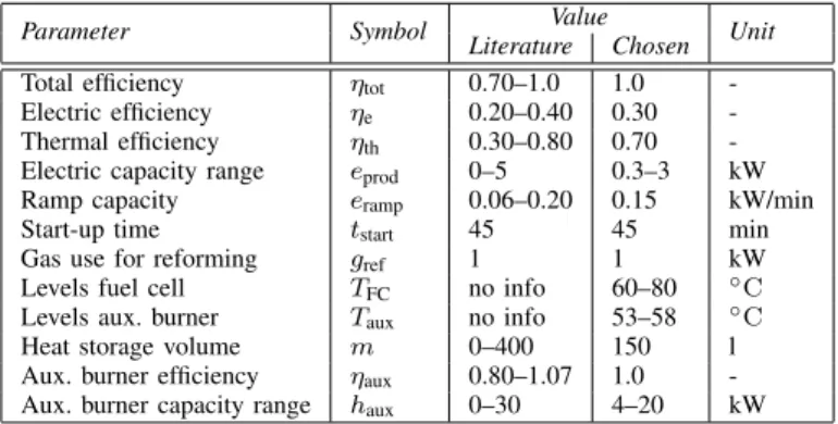
The parameter values mentioned in the literature and chosen here for the models are shown in Table I. As will be explained further in Section II-B2, in heat-led control the micro-CHP prime mover and auxiliary burner are (de)activated according to temperature levels of the water in the storage (i.e.TFC,Taux). There are minimum and maximum temperature levels defined for the prime mover as well as for the auxiliary burner. Values for these temperature levels have been chosen by the authors based on expert knowledge from boiler manufacturers.
2) Design of the heat-led controller: In heat-led control the micro-CHP system’s power output is controlled based on domestic heat demand. We next describe the heat-led control strategy applied to the PEMFC system.
The temperature of the water in the heat storage functions as main control parameter in the strategy. The prime mover output is controlled such as to keep the storage temperature at an average value Ta of:
Ta= (Tlow,FC+Thigh,FC)/2 = 70◦C, (7) corresponding with an average energy level denoted by hs,a. The values for Tlow,FC and Thigh,FC are given in Table I. The auxiliary burner control is also based on the storage
TABLE I
MODEL PARAMETERS FORPEMFCAND AUXILIARY BURNER(‘NO INFO’ MEANS THAT NO INFORMATION WAS FOUND IN THE LITERATURE ON THIS PARAMETER, ‘AUX.BURNER’STANDS FOR AUXILIARY BURNER). BASED
ON DATA FROM[25]–[31].
Parameter Symbol Value Unit
Literature Chosen
Total efficiency ηtot 0.70–1.0 1.0
-Electric efficiency ηe 0.20–0.40 0.30
-Thermal efficiency ηth 0.30–0.80 0.70
-Electric capacity range eprod 0–5 0.3–3 kW
Ramp capacity eramp 0.06–0.20 0.15 kW/min
Start-up time tstart 45 45 min
Gas use for reforming gref 1 1 kW
Levels fuel cell TFC no info 60–80 ◦C
Levels aux. burner Taux no info 53–58 ◦C
Heat storage volume m 0–400 150 l
Aux. burner efficiency ηaux 0.80–1.07 1.0
-Aux. burner capacity range haux 0–30 4–20 kW
physical system aux , h start,r , t heat−led controller hs hFC
Fig. 3. The heat-led controller in relation to the micro-CHP unit that it controls.
temperature level. The corresponding energy levels of the heat storage at simulation step k are calculated from the temperatures with:
hs[k] =m[k]c∆T[k], (8) where m[k] is the mass of the water in the storage at time stepk,c is the specific heat of water (i.e. 4.18 kJ/(kg·K)) and ∆T[k]is the difference between the storage temperature and the temperature of the environment (Tenv = 20◦C) at time step k. Figure 3 schematically illustrates the control inputs the heat-led controller requires and the outputs the controller sends to the micro-CHP system. The interpretation of the state variabletstart,r[k], which the controller measures at each time stepk(together with the heat storage energy contenths), and the decision variableshFCandhaux, which the controller sends to the system it controls, will be given below.
To avoid frequent starting up of the system, the control strategy is aimed at keeping the prime mover in operation as long as possible. In reality, heat and electricity are con-sumed by households continuously. Here, energy consumption is modeled by assigning values for domestic heat demand hd[k] and electricity demand ed[k] each simulation step k. The controller takes this information on energy demand into account to determine its actions at each time step k. The heat demand is taken from the heat storage, which thereby decreases in temperature. The heat storage contenths[k]is also an input for the controller. The thermal power output hFC[k] of the PEMFC prime mover is controlled according to:
hFC[k] =
max hs,a−hs[k] +hd[k], hFC,min
if (tstart,r[k−1] = 1)∨ (hFC[k−1]>0) ∧(hs[k]−hd[k] +hFC,min< hhigh,FC)
0 otherwise,
(9) where tstart,r[k] is the remaining start-up time at time step k. The PEMFC’s thermal capacity hFC[k] should be as low as possible, respecting the capacity limits given by (3) and the power ramp rate constraint (5). The remaining start-up time is
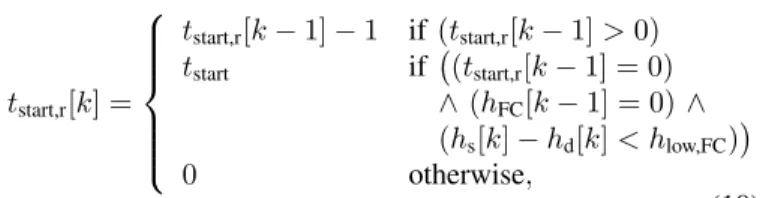
set by the controller according to: tstart,r[k] = tstart,r[k−1]−1 if (tstart,r[k−1]>0) tstart if (tstart,r[k−1] = 0) ∧(hFC[k−1] = 0)∧ (hs[k]−hd[k]< hlow,FC) 0 otherwise, (10) where tstart is the start-up time in 15-minute time steps from Table I (i.e., tstart = 3). The controller thus also needs information from the prime mover on the remaining start-up time at the previous time stepk−1. During start-up of the fuel cell heat can be extracted from the storage, thereby lowering the storage temperature. In order to avoid using the auxiliary burner, the activation temperature for the fuel cell is therefore set relatively high (i.e.,Tlow,FC> Thigh,aux).
Using (9) a new intermediate value for the energy storage content is calculated by the controller with:
hs,new[k] =hs[k]−hd[k] +hFC[k]. (11) Even if the fuel cell prime mover is running, the heat storage may still become too cold and its temperature may drop below Tlow,aux. In that case the auxiliary burner will be activated by the controller using (11) according to:
haux[k] =
max(hhigh,aux−hs,new[k], haux,min) if(hs,new[k]< hlow,aux)
0 otherwise.
(12) The auxiliary burner capacity haux[k] should be set by the controller as low as possible and stay between the limits given by (5). The desired burner capacity is such that the storage can reach temperatureThigh,aux, which is the maximum temperature to which the auxiliary burner can heat the storage.
The controller is designed to let the fuel cell shut down completely when the storage reaches the temperature limit Thigh,FC and to let the fuel cell go through the start-up time before being able to produce usable energy again. The gas used during start-upgr[k]follows from:
gr[k] =
gref if tstart,r[k]>0
0 otherwise, (13)
withgrefbeing the gas used for reforming during start-up (see Table I).
The new value for the energy storage content, with which the next simulation step starts, follows from (6). With (1) and (2) values for eimp[k] andeexp[k] are calculated.
3) Model input: The model of the controller that has just been described requires energy demand as input. To calculate the economic performance of the micro-CHP system, price data is also needed. This section describes the input data that we will use in the subsequent section in simulations. The Dutch situation of 2006 is used as the source of the data.
a) Energy demand profiles: According to [32], domes-tic energy demand profiles can be constructed based on measurements [15], [23], from the aggregation of individual component loads [33], or by using stochastic methods [34]. Here the last approach is taken, based on the following steps:
1) Set the annual electricity and heat demand in kWh.
2) Create average profiles by multiplying the annual de-mand by certain fractions. This allocates the annual demand to a demand per 15-minute periods for a full year.
3) For each time step, take a sample from a probability distribution around the 15-minute demand value. In the analysis of this paper average households are used with regard to their annual electricity and heat demand. An average annual domestic electricity demand of 3,400 kWh [8] and an average annual domestic heat demand of 12,500 kWh [35] are taken. This heat demand is the total demand for space heat and domestic hot water. To createaveragedomestic electricity and heat demand profiles, the annual demands are multiplied by the so-called ‘profile fractions’ from [36]. These profile fractions are used by Dutch market parties to predict the electricity and gas demand of small consumers. The heat profiles initially have a resolution of one hour (equal to the resolution of the gas profiles) and the electricity profiles of 15 minutes. The hourly heat demand data are split into equal amounts for 15-minute periods to create the same resolution as for the electricity profiles.
In constructingindividualdomestic electricity demand pro-files, at each 15-minute time period a sample is taken from an exponential distribution, in which the expected value is equal to the average electricity demand at that time. With an exponential distribution the large spikes in domestic electric-ity demand can be simulated quite accurately compared to empirical data from [21], [34], [37]. In creating individual domestic heat demand profiles, samples are taken from normal distributions, with the expected values equaling the average heat demand at that time period. Normal distributions are more suitable for simulating the heat demand, as the demand spikes are much smaller than with electricity [34]. By using gas demand profile fractions it is assumed that the daily patterns of gas and heat consumption are equal. As still only 15 % of Dutch households presently have hot water storage systems [35], regarding gas demand as heat demand seems a valid assumption. In creating profiles for the aggregate heat demand, standard deviations are chosen so as to get maximum peaks in the total thermal power demand that approximate numbers mentioned in [21], [34] as well as possible.
Figure 4 shows examples of individual domestic electricity and heat load profiles together with the average profiles.
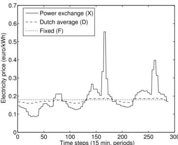
b) Price data: Regarding the electricity price for house-holds, we assume that so-called smart meters will enable real-time pricing. Then, instead of having flat rates, prices can vary in time. Real-time prices will be based on marginal supply costs for an energy company [38]. Marginal energy costs at a certain moment depend on prices of power pools and power exchanges, costs of own power generation, and costs of bilateral transactions [38]. For the modeling work of this paper, we assume three electricity tariff structures for trading electricity, namely: fixed tariffs (denoted byF), real-time pricing based on Dutch power exchange prices (hourly resolution; denoted by X), and real-time pricing reflecting average Dutch wholesale market prices (varying with a 15-minute resolution; denoted by D). The construction of these tariff structures is as follows:
0 50 100 150 200 250 300 0 1 2 3 4 5 6
Time steps (15 min. periods)
Electricity demand (kW)
Constructed Average aggregate
(a) Electricity demand.
0 50 100 150 200 250 300 0 1 2 3 4 5 6 7 8 9 10
Time steps (15 min. periods)
Heat demand (kW)
Constructed Average aggregate
(b) Heat demand.
Fig. 4. Examples of constructed energy demand profiles for the first three days of January 2006.
• F tariff structure. From [8], [9] a residential tariff of
0.18 C/kWh is obtained (this is the variable part of the tariff including taxes), which is used in theF structure.
• X tariff structure. According to [8] the supply part of
the residential tariff (including taxes) is 0.09 C/kWh. The rest of the C0.18 consists of the transport part (i.e., C0.04) and taxes (i.e., C0.05). In creating the hourly-varying tariff structure, the supply part of 0.09 C/kWh is substituted by an hourly-varying supply tariff. For the X structure the hourly-varying supply tariff is equal to prices of the Dutch Amsterdam Power Exchange (APX), which is a day-ahead market [39]. It is hereby assumed that the retailer is able to buy and sell all the power for and from households on the APX. So, all the supply and demand bids that he places on the APX are accepted. This implicitly assumes that retailers can predict the net consumption of their domestic customers.
• D tariff structure. In setting real-time pricing tariffs for
domestic customers, energy retailers can alternatively use
0 50 100 150 200 250 300 0 0.1 0.2 0.3 0.4 0.5 0.6 0.7
Time steps (15 min. periods)
Electricity price (euro/kWh)
Fixed (F) Dutch average (D) Power exchange (X)
Fig. 5. The three residential electricity tariff structures that are used in the simulations, for the first three days of January 2006.
a mixture of the prices on all the electricity markets on which they trade [38]. In the Netherlands, for example, only 20 % of all power is traded on the APX [40] and a mixture of prices seems logical then. In creating the varying supply tariff for theDstructure, a merit order of Dutch generation facilities based on marginal costs (as described in [40]), together with national load data from the Dutch transmission system operator [41] are used. The Dutch electricity system is thereby conceptualized as a black-box and all electricity is assumed to be traded through one ‘average’ market.
The residential electricity tariffs are scaled such that the annual averages of the three tariff structures are equal. In Figure 5 the three constructed tariff structures are shown for three days in January 2006. It can be clearly seen that theX structure is more erratic than theD structure.
In determining the tariffs for electricity that is sold by a household to the energy retailer, i.e., the feedback tariff, the following is considered. It is first of all assumed that there is an electricity transport tariff per kWh of electricity sold. A zero feed-back tariff for exported electricity is highly improbable, as energy retailers will have free electricity at their disposal then. On the other hand, households with PEMFCs produce so much electricity themselves, that they can easily become net-producers of electricity (in, say, a period of a year). Feed-back tariffs that are equal to import tariffs are illogical then, as households would then incur net transport revenues. A nonzero feed-back tariff is considered, which comprises the previously mentioned supply part and further prevents double-taxation on energy. The feed-back tariffs then become equal to the import tariffs minus the transport tariff of 0.04 C/kWh.
For gas, from [8], [9] a variable domestic tariff (including taxes) of 0.06 C/kWh is used.
C. Economic performance with heat-led control
In this section we analyze the economic situation of house-holds in which micro-CHP systems are controlled in a heat-led
TABLE II
ANNUAL ENERGY COSTS FOR CONVENTIONAL HOUSEHOLDS,DEPENDING ON THE TARIFF STRUCTURE.
Total energy costs ( C/y) Of which gas ( C/y)
F X D
1,317 1,350 1,324 714
TABLE III
ANNUAL ENERGY COSTS WITHPEMFCMICRO-CHPUNDER HEAT-LED CONTROL,DEPENDING ON THE TARIFF STRUCTURE AND GIVEN AS A
PERCENTAGE OF THE COSTS OF CONVENTIONAL HOUSEHOLDS. Total energy costs (% of conventional) Gas
F X D (%)
61 61 62 144
way. We do this by implementing the mathematical models of the household-retailer system and the heat-led controller in Matlab 7.5 and performing simulations in which the input data described above are used.
Multiple simulations with equivalent households but with different electricity and heat demand profiles were done. The households each have a heat storage volume of 150 liters. At the start of each simulation, the micro-CHP units are not running (i.e., hprime = 0kW and haux = 0kW) and the heat storages all have average energy levels. The electricity and heat demand profiles were created as explained in Section II-B3. Each load profile of a household consists of 35,040 data points, as simulations are done over a full year (i.e., 2006) and pro-files have a 15-minute resolution. The economic performance of micro-CHP application under different tariff structures is obtained using 20 simulations. Experiments have confirmed that this number is high enough to draw statistically significant conclusions.
To place the results that are discussed in the subsequent sec-tions in perspective, first annual energy costs for conventional households are shown in Table II. Table III gives the annual energy costs of the heat-led case as a percentage of the costs of conventional households (Table II). The presented numbers in both tables are the average values per tariff structured over all simulations.
The following observations are made from Table III regard-ing domestic energy costs in the heat-led case:
• Substantial cost savings with micro-CHP compared
to conventional households. Relative cost savings are almost 40 %.
• Higher gas costs for micro-CHP households. To
pro-duce the same amount of thermal energy, a micro-CHP unit will consume more gas than a conventional condens-ing boiler. This can be seen by the higher gas costs for households with micro-CHP compared to conventional households. Even though micro-CHP application leads to higher local gas consumption in households, the total primary energy consumption for which households are responsible becomes less with micro-CHP.
Now that the reference case has been analyzed, the follow-ing section looks into the potential further cost reductions with
demand response.
III. ENHANCED ECONOMIC FEASIBILITY THROUGH DEMAND RESPONSE
Instead of following domestic heat demand, the flexibility provided by the micro-CHP and storage systems can be used more actively and intelligently, without compromising comfort for households in terms of heat demand. In this section we propose a more intelligent control strategy to enhance the economic savings with micro-CHP systems, when compared to the heat-led case as analyzed before. The proposed scheme fo-cuses on reducing variable energy costs via demand response. Demand response with micro-CHP is reported in [21], [42]– [49]. In [21], [45], [48] cost savings compared to standard heat-led control are mentioned. Relative savings between 2 to 8 % are reported in those studies. In the existing literature the influence of tariff structures on cost savings with demand response and the design of the controllers is not looked into. This section does address the influence of the tariff structure and the controller design.
In the following sections we first formulate the controller that focuses on demand response with micro-CHP and then we analyze its performance.
A. Model predictive control (MPC)
The control strategy that is proposed here for demand response is model predictive control (MPC) [50]–[52]. An MPC controller is connected to or is built into the micro-CHP unit. It is also connected to the storage system and a smart meter. The presence of smart metering in households is assumed in order for price information to be conveyed to households by the retail company.
The controller has the task to determine how the micro-CHP system should operate and how heat should be supplied to the heat storage. The controller thereby has the objective to minimize the variable energy costs while respecting the oper-ational constraints. The concept of MPC is shown in Figure 6. The MPC control agent uses a model of the household-retailer system to determine the optimal control actions. Below it is further discussed how MPC is applied to the system under study.
1) MPC framework: To find the actions that meet control objectives as well as possible, a controller has to make a trade-off between different possible actions. In order to make the best decision, as much relevant information about the conse-quences of choosing actions as possible should be taken into account. A particularly useful form of control that in principle can use all information available is MPC [50]–[52]. MPC is an optimization-based control technique, which over the last decades has shown successful application in the process industry [54] and which is now gaining increasing attention in fields like road traffic networks [55], steam networks [56], water networks [57], and also power networks [58], [59].
Here MPC is used as the control strategy for demand response with micro-CHP. There are distinct and predictable patterns in domestic energy demand and energy market prices of which predictive control is expected to be able to take
of system state measurement physical system actions optimizer model control agent desired behavior constraints
Fig. 6. The concept of MPC (adapted from [53]).
advantage. The controller uses an MPC strategy such that it can:
• take into account the decision freedom due to the
possi-bilities of self-generation of electricity and of electricity import and export;
• optimize the use of the heat storage unit;
• incorporate predictions of domestic electricity and heat
demand and future information on electricity prices (i.e., disturbances);
• incorporate models of the dynamics and constraints of
installed energy conversion and storage units.
2) MPC components: MPC is a control strategy that is typically used in a discrete-time control context. At each time step, an optimization problem is solved with the following components:
• an objective functionexpressing which system behavior
and actions are desired;
• aprediction modeldescribing the behavior of the system
subject to actions;
• possibleconstraintson the states, the inputs, and the
out-puts of the system (where the inout-puts and the outout-puts of the system correspond to the actions and the measurements of the controller, respectively);
• possible known information about futuredisturbances; • ameasurementof the state of the system at the beginning
of the current control cycle.
The objective of the controller is to determine those actions that optimize the behavior of the system as specified in an objective function.
B. MPC problem formulation
1) Objective function: The control objective is to minimize the variable costs of domestic energy use. These costs depend on the gas price pg, the price of imported electricity pimp, and the price of exported electricity pexp. The gas price is considered to be fixed over time and the evolution of pimp and pexp depends on the applied tariff structure as discussed in Section II-B3.
The cost functionJ at time stepkover a prediction horizon with lengthN is now defined as:
J = N−1 X l=0 pg gFC[k+l] +gaux[k+l] +gr[k+l]
+pimp[k+l]eimp[k+l]−pexp[k+l]eexp[k+l]
. (14)
2) Prediction model and operational constraints: The pre-diction model and operational constraints that the controller uses consist of a set of relations describing the household-retailer system. This set of relations makes up a mathematical model that builds upon the model of Section II-B1 and is a further elaboration of the model presented in [60]. Parts of the model equations have already been given in Section II-B1. All the model parameters are given in Table I.
The main difference between the heat-led strategy and the demand response strategy is that now the micro-CHP controller sets the power output of the micro-CHP system (i.e.hFCandhaux) by only considering costs, while with heat-led control the power output was set to keep the storage temperature at its average value. The main constraints are on the power output, which should remain within the operational limits, and on the temperature of the water in the heat storage, which should remain between the minimum and maximum limits. It is assumed that the temperature of the water in the heat storage should remain between Tmin = 55◦C and
Tmax= 80◦C.
Now the mathematical model of household-retailer system will be described. First the binary variablesvCHP[k]andvaux[k], which indicate whether the micro-CHP prime mover and auxiliary burner are in operation at a specific time step k, are defined according to:
vCHP[k] =
1 if micro-CHP prime mover operates
0 if micro-CHP prime mover does not operate, vaux[k] =
1 if auxiliary burner operates
0 if auxiliary burner does not operate. In addition, the binary variables that indicate whether the micro-CHP prime mover and the auxiliary burner start up or shut down at time stepk are defined as:
uCHP,up[k] =
1 if prime mover starts up
0 if prime mover does not start up, uCHP,down[k] =
1 if prime mover shuts down
0 if prime mover does not shut down, uaux,up[k] =
1 if auxiliary burner starts up
0 if auxiliary burner does not start up, uaux,down[k] =
1 if auxiliary burner shuts down
As also shown in (3) the power output of the prime movereprod[k]can modulate between a certain minimum and maximum capacity, which is now modeled by:
vCHP[k]eprod,min≤eprod[k]≤vCHP[k]eprod,max, (15) where eprod,min andeprod,max are the minimum and maximum electric capacity.
With the binary variables introduced above, the auxiliary burner power output rangehaux[k] is now given by:
vaux[k]haux,min≤haux[k]≤vaux[k]haux,max. (16) The thermal energy in the heat storage hs[k] has to stay between a minimum and maximum value:
hs,min≤hs[k]≤hs,max. (17)
The values ofhs,min andhs,max are calculated with (8) using
the temperatures mentioned above.
The energy content of the heat storage hs[k] changes over time due to the consumption and generation of heat. The dynamics of the heat storage is given in (6). Also equations (4), (2), and (1) will hold.
As said before, the fuel cell system has a certain start-up time during which it consumes gas but delivers no usable electricity and heat. The system start-up is modeled by:
vCHP[k+p]≥uCHP,up[k], p= 0, . . . , tstart−1, (18) wheretstartis the start-up time expressed in 15 minute periods. Furthermore, the following statement is also needed to ensure that there is no electricity production during start-up:
if uCHP,up[k] = 1theneprod[k+q] = 0,
q= 0, . . . , tstart−1, (19) which can be modeled as a mixed-integer linear programming problem [61]. Gas that is used during start-up to heat up the reformer is represented by the variablegr[k](see Figure 2). As was also done with (13), the following relation ensures that the total gas consumption of the fuel cell will not be lower thangrefwhen the fuel cell is starting up:
gr[k] =
gref if vCHP[k] = 1∧gFC[k] = 0
0 otherwise. (20)
In order to let the micro-CHP’s prime mover and auxiliary burner function properly, the model should include equations that link the binary variables that govern the operation of the prime mover and the burner:
vCHP[k]−vCHP[k−1] =uCHP,up[k]−uCHP,down[k] (21)
vaux[k]−vaux[k−1] =uaux,up[k]−uaux,down[k] (22)
uCHP,up[k] +uCHP,down[k]≤1 (23)
uaux,up[k] +uaux,down[k]≤1. (24)
3) MPC scheme: At the beginning of each time step k, the controller measures the system state of the previous step, which consists of values of the heat storage energy level hs and of the binary variablesvCHP andvaux (these are the state variables). Due to the constraining ramp rate on the fuel cell’s power output, the electricity that was produced in the previous step,eprod, is also measured. Further, between time steps the start-up time of the PEMFC tstart should also be taken into account.
Then, together with data on future energy consumption and electricity prices the controller then determines values for the decision variables gFC, gaux, gr, eexp,and eimp. It does so by minimizing the objective function over a prediction horizon with length N, subject to the prediction model and the initial system state. Hence, a large set of mixed-integer, linear equality and inequality constraints has to be solved. A prediction horizon of 96 steps is taken (i.e., N = 96, which equals one day). This horizon length covers the dynamics of domestic energy demand and the electricity market.
Once the controller has determined the actions that optimize the system performance over the prediction horizon, it imple-ments the actions of the first step of the horizon k until the beginning of the next time stepk+ 1.
At the start of time step k+ 1 the procedure is repeated: the controller determines new optimal actions over the shifted prediction horizon that now starts at k+ 1, thereby using new system measurements and updated information on distur-bances. Hence, the controller operates in a receding or rolling horizon fashion to determine its actions.
4) Solving the optimization problem: The MPC optimiza-tion problem is formulated as a mixed-integer linear pro-gramming problem. It is linear, since the objective function and all constraints are linear and it is mixed-integer, since the problem involves continuous and binary variables. There are optimization solvers available that can deal with these kind of optimization problems [62]. In the case study the optimization problems are solved using the ILOG CPLEX [63] linear mixed-integer programming solver through the Tomlab interface [64] in Matlab. To give an idea of the size of the optimization problems: with a prediction horizon of 96 steps (i.e., one day), at each time step an optimization problem consisting of around 2,500 equations and 1,200 variables (continuous and binary) has to be solved. Solving such an optimization problem with the used solver takes from about a few seconds to about a minute on a laptop with a 1.9 GHz CPU and 1.0 GB internal memory.
5) Prediction accuracy of energy demand and prices: The energy demand profiles and the electricity prices that the MPC controller uses are assumed to be perfectly known to the controller. Energy demand profiles can be determined by the controller itself or by an external device. Forecasted prices are conveyed to households by their retailer, who provides this information as a service. By assuming perfect forecasts on prices and energy demand, this analysis gives an upper limit on the potential savings with demand response. The domestic energy demand profiles and electricity tariff structures used are described in Section II-B3.
10 20 30 40 50 60 70 80 90 6 6.5 7 7.5 8 8.5 9 9.5 10 10.5 11
Time steps (15 min. periods)
hs
(k
Wh
)
Fig. 7. Evolution over a day of the heat storage content of one household.
10 20 30 40 50 60 70 80 90 0 0.1 0.2 0.3 0.4 0.5 0.6 0.7 0.8
Time steps (15 min. periods)
E le ct ri ci ty ex ch an g e w it h th e g ri d (k Wh ) eexp eimp
Fig. 8. Evolution over a day of the electricity import and export of one household.
C. Additional savings with demand response
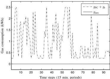
In this section the energy costs with MPC applied to PEMFC micro-CHP systems are determined and a comparison with the results with heat-led control is made. The same households are considered as in Section II (in terms of pa-rameters and energy demand patterns), only now the domestic heating system is controlled by an MPC controller instead of the heat-led controller. As an illustration of the typical behavior of the households, Figures 7, 8, and 9 show the evolution over the first day of the simulation of the state of the heat storage, the electricity import and export, and the gas consumption of the micro-CHP’s prime mover and auxiliary burner, respectively. The aggregate energy cost savings with MPC under the different tariff structures compared to heat-led control are shown in Table IV.
The results show that, compared to heat-led operation, additional cost savings with demand response are between 9– 112 C/year, or between 1–14 %. The savings strongly depend on the tariff structure. TheXtariff structure shows the highest savings and the F structure the lowest. MPC control reduces costs by shifting net-consumption away from moments of high prices. Because theX tariff structure is based on the real-time
10 20 30 40 50 60 70 80 90 0 0.5 1 1.5 2 2.5
Time steps (15 min. periods)
G as co n su m p ti o n (k Wh ) gFC+gr gaux
Fig. 9. Evolution over a day of the gas consumption of the prime mover and auxiliary burner of one household.
TABLE IV
ABSOLUTE AND RELATIVE ENERGY COST SAVINGS WITH DEMAND RESPONSE OFPEMFCMICRO-CHPSYSTEMS,DEPENDING ON THE TARIFF
STRUCTURE AND COMPARED TO HEAT-LED CONTROL. Cost saving with MPC under specific pricing regime Absolute ( C/year) Relative to heat-led control (%)
F X D F X D
8.9 111.6 20.2 1.1 13.6 2.5
prices with the highest variation, it is logical that MPC can create most savings with that structure.
IV. CONCLUSIONS AND FUTURE RESEARCH
In the development towards more energy efficiency, a promising option is the application of micro combined heat and power systems (micro-CHP) in households. Micro-CHP systems simultaneously generate heat and power and thereby improve energy efficiency and reduce carbon emissions. Com-pared to wind turbines and photovoltaic systems, micro-CHP is a special type of distributed generation technology in the sense that the power output of the system can be controlled. Further, when micro-CHP units are coupled to heat storage systems, flexibility in their power generation can be created.
Flexibility in power generation can lead to energy cost sav-ings. The amount of these savings depends on how micro-CHP systems will be applied once being installed in households. Higher savings may be obtained by controlling micro-CHP systems more intelligently. An objective to which intelligent control with micro-CHP can be directed is demand response. In the context of this paper, demand response is the ability of households to change their electricity net-consumption in response to real-time prices. In this paper we have analyzed the potential economic value of demand response with fuel cell micro-CHP systems. Due to their relatively low heat-to-power ratio compared to other prime mover technologies, fuel cells will provide the highest level of flexibility. The micro-CHP units modeled in this paper use a Proton Exchange Membrane Fuel Cell (PEMFC) as prime mover.
First the economics of standard application of micro-CHP were analyzed. The most logical standard control strategy for micro-CHP systems is heat-led control, in which the micro-CHP’s power output follows heat demand. With heat-led control annual energy costs are reduced with around 40 %, compared to when households would use conventional gas boilers. As a next step the additional energy cost savings with demand response, compared to heat-led control, were calculated. Demand response was implemented in a model predictive control (MPC) strategy. With demand response vari-able energy costs are between 1–14 % lower than with heat-led control. Absolute savings with demand response compared to heat-led control are about C9–112 per year per household. Cost savings with demand response strongly depend on the structure of the real-time electricity tariffs: with more strongly fluctuating structures more savings can be earned.
Future research should further extend the assessment of the performance of the MPC strategy proposed here by quan-tifying the relation between the economic performance and the inherent uncertainty in demand profiles and prices, and by considering a larger range of household types in terms of electricity and heat demand (which could include also adaptive electric and heat loads). The results of this paper represent an upper limit in potential savings that can be achieved, because perfect energy demand predictions were assumed to be used by the MPC controller. In addition, besides real-time prices for electricity, also real-time prices for gas should be included in the MPC scheme, and the robustness of the conclusions to the difference in price between electricity and gas should be studied. Furthermore, as cost savings with intelligent control should also cover the investments in that intelligence, the costs of MPC controllers should be looked into. MPC applied to prime movers with a higher heat-to-power ratio than fuel cells (i.e. Stirling engines and internal combustion engines) will provide a lower degree of operational flexibility and therefore lower absolute savings with demand response. How much lower these savings will be can be further researched as well. Further, the impact of different PEMFC capacities and different heat storage volumes on cost savings with demand response should be further researched.
The magnitude of the savings that can be achieved with demand response do not provide a very strong incentive to individual households to undertake demand response with their micro-CHP unit. Demand response could also be applied to clusters of micro-CHPs in virtual power plants (VPPs) [65]. Then, small savings of per household can provide an
aggregate economic incentive to set up a VPP. Applying demand response in VPPs is recommended as future research as well.
ACKNOWLEDGMENTS
This research is supported by the BSIK project “Next Generation Infrastructures (NGI)”, the Delft Research Center Next Generation Infrastructures, and the European STREP project “Hierarchical and distributed model predictive control (HD-MPC)”. The authors would like to thank the reviewers for their useful comments and feedback.
REFERENCES
[1] “IEA – World Energy Outlook,” URL: http://www.worldenergyoutlook. org/.
[2] T. J. Hammons, “Integrating renewable energy sources into European grids,” International Journal of Electrical Power & Energy Systems, vol. 30, no. 8, pp. 462–475, October 2008.
[3] N. Jenkins, R. Allan, P. Crossley, D. Kirschen, and G. Strbac,Embedded Generation. London, UK: The Institution of Electrical Engineers, 2000, vol. 31.
[4] A. Chambers, S. Hamilton, and B. Schnoor,Distributed Generation: A Nontechnical Guide. Tulsa, Oklahoma: Penn Well Corporation, 2001. [5] J. A. Pec¸as Lopes, N. Hatziargyriou, J. Mutale, P. Djapic, and N. Jenk-ins, “Integrating distributed generation into electric power systems: A review of drivers, challenges and opportunities,”Electric Power Systems Research, vol. 77, no. 9, pp. 1189–1203, July 2007.
[6] A. M. Borbely, R. Brent, J. Brouwer, S. Cherian, and P. S. Curtiss, Distributed Generation: The Power Paradigm for the New Millennium. Boca Raton, Florida: CRC Press LLC, 2001.
[7] N. Hatziargyriou, H. Asano, R. Iravani, and C. Marnay, “Microgrids: An overview of ongoing research, development, and demonstration projects,” IEEE Power & Energy Magazine, vol. 5, no. 4, pp. 78–94, 2007.
[8] “Energy Research Centre of The Netherlands (ECN),” URL: http://www. energie.nl/, 2009.
[9] CBS, “Statistics Netherlands,” URL: http://www.cbs.nl/, 2009. [10] M. Pehnt, M. Cames, C. Fischer, B. Praetorius, L. Schneider, K.
Schu-macher, and J. Vob,Micro Cogeneration: Towards Decentralized Energy Systems. Berlin, Germany: Springer, 2006.
[11] R. Beith, I. P. Burdon, and M. Knowles, Micro Energy Systems: Review of Technology, Issues of Scale and Integration. Suffolk, UK: Professional Engineering Publishing Limited, 2004.
[12] WhisperTech, URL: http://www.whispergen.com/, 2009. [13] CeresPower, URL: http://www.cerespower.com/, 2009.
[14] A. D. Peacock and M. Newborough, “Controlling micro-CHP systems to modulate electrical load profiles,”Energy, vol. 32, no. 7, pp. 1093–1103, July 2007.
[15] ——, “Effect of heat-saving measures on the CO2savings attributable to micro-combined heat and power (mCHP) systems in UK dwellings,” Energy, vol. 33, no. 4, pp. 601–612, April 2008.
[16] J. E. Brown, C. N. Hendry, and P. Harborne, “An emerging market in fuel cells? Residential combined heat and power in four countries,”Energy Policy, vol. 35, no. 4, pp. 2173–2186, April 2007.
[17] D. Haeseldonckx, L. Peeters, L. Helsen, and W. D’haeseleer, “The im-pact of thermal storage on the operational behaviour of residential CHP facilities and the overall co2 emissions,” Renewable and Sustainable Energy Reviews, vol. 11, no. 6, pp. 1227–1243, August 2007. [18] D. Pudjianto, C. Ramsay, and G. Strbac, “Virtual power plant and
system integration of distributed energy resources,” IET Renewable Power Generation Journal, vol. 1, no. 1, pp. 10–16, March 2007. [19] ——, “Microgrids and virtual power plants: concepts to support the
in-tegration of distributed energy resources,”Proceedings of the Institution of Mechanical Engineers, Part A: Journal of Power and Energy, vol. 222, no. 7, pp. 731–741, 2008.
[20] J. B. Cardell, “Distributed resource participation in local balancing energy markets,” inProceedings of IEEE PowerTech, Lausanne, Switzer-land, July 2007.
[21] A. D. Hawkes and M. A. Leach, “Cost-effective operating strategy for residential micro-combined heat and power,”Energy, vol. 32, no. 5, pp. 711–723, May 2007.
[22] A. D. Peacock and M. Newborough, “Impact of micro-combined heat-and-power systems on energy flows in the UK electricity supply indus-try,”Energy, vol. 31, no. 12, pp. 1804–1818, September 2006. [23] ——, “Impact of micro-CHP systems on domestic sector CO2
emis-sions,”Applied Thermal Engineering, vol. 25, no. 17-18, pp. 2653–2676, December 2005.
[24] M. Newborough, “Assessing the benefits of implementing micro-CHP systems in the UK,” Proceedings of the Institution of Mechanical Engineers, Part A: Journal of Power and Energy, vol. 218, no. 4, pp. 203–218, August 2004.
[25] I. Staffell, R. Green, and K. Kendall, “Cost targets for domestic fuel cell CHP,”Journal of Power Sources, vol. 181, no. 2, pp. 339–349, July 2008.
[26] H. I. Onovwionaa and V. I. Ugursalb, “Residential cogeneration systems: Review of the current technology,”Renewable and Sustainable Energy Reviews, vol. 10, no. 5, pp. 389–431, October 2006.
[27] Y. Hamada and M. Nakamura, “Field performance of a polymer electrolyte fuel cell for a residential energy system,”Renewable and Sustainable Energy Reviews, vol. 9, no. 4, pp. 345–362, August 2005. [28] M. W. Davis, A. Hunter Fanney, M. J. LaBarre, K. R. Henderson, and
B. P. Dougherty, “Parameters affecting the performance of a residential-scale stationary fuel cell system,” Journal of Fuel Cell Science and Technology, vol. 4, no. 2, pp. 109–115, 2007.
[29] S. Obara, “Dynamic characteristics of a PEM fuel cell system for individual houses,”International Journal of Energy Research, vol. 30, no. 15, pp. 1278–1294, August 2006.
[30] C. Wallmark and P. Alvfors, “Design of stationary PEFC system configurations to meet heat and power demands,” Journal of Power Sources, vol. 106, no. 1, pp. 83–92, April 2002.
[31] M. Dentice d’Accadia, M. Sasso, S. Sibilio, and L. Vanoli, “Micro-combined heat and power in residential and light commercial applica-tions,”Applied Thermal Engineering, vol. 23, no. 10, pp. 1247–1259, July 2003.
[32] V. Dorer and A. Weber, “Energy and CO2emissions performance assess-ment of residential micro-cogeneration systems with dynamic whole-building simulation programs,” Energy Conversion and Management, vol. 50, no. 3, pp. 648–657, March 2008.
[33] D. H. O. McQueen, P. R. Hyland, and S. J. Watson, “Monte Carlo simulation of residential electricity demand for forecasting maximum demand on distribution networks,”IEEE Transactions on Power Systems, vol. 19, no. 3, pp. 1685–1689, August 2004.
[34] P. C. van der Laag and G. J. Ruijg, “Micro-warmtekrachtsystemen voor de energievoorziening van Nederlandse huishoudens (Micro-CHP systems for the energy supply of The Netherlands),” Energy Research Centre of the Netherlands (ECN), Petten, The Netherlands, Tech. Rep. ECN-C-02-006, September 2002, in Dutch.
[35] A. de Jong, E. J. Bakker, J. Dam, and H. van Wolferen, “Tech-nisch energie- en CO2-besparingspotentieel van micro-wkk in nederland (2010–2030) (Technical energy and CO2 reduction potential of micro-CHP in The Netherlands (2010–2030)),” Platform Nieuw Gas, Tech. Rep., July 2006, in Dutch.
[36] EnergieNed, URL: http://www.energiened.nl.
[37] P. J. Boait, R. M. Rylatt, and M. Stokes, “Optimisation of consumer benefits from microcombined heat and power,”Energy and Buildings, vol. 38, no. 8, pp. 981–987, August 2006.
[38] G. Barbose, C. Goldman, and B. Neenan, “A survey of utility experience with real time pricing,” Lawrence Berkeley National Laboratory: Envi-ronmental Energy Technologies Division, Berkeley, CA, USA, Tech. Rep. LBNL-54238, December 2004.
[39] APX, URL: http://www.apxgroup.com, 2009.
[40] L. J. de Vries, “Securing the public interest in electricity generation markets; the myths of the invisible hand and the copper plate,” Ph.D. dissertation, Delft University of Technology, Delft, The Netherlands, Juni 2004.
[41] TenneT, URL: http://www.tennet.nl/, 2009.
[42] X. Q. Kong, R. Z. Wang, Y. Li, and X. H. Huang, “Optimal operation of a micro-combined cooling, heating and power system driven by a gas engine,”Energy Conversion and Management, vol. 50, no. 3, pp. 530–538, March 2009.
[43] A. M. Azmy and I. Erlich, “Online optimal management of PEM fuel cells using neural networks,” IEEE Transactions on Power Delivery, vol. 20, no. 2, pp. 1051–1058, April 2005.
[44] A. M. Azmy, M. R. Mohamed, and I. Erlich, “Decision tree-based approach for online management of fuel cells supplying residential loads,” inProceedings the IEEE PowerTech Conference, St. Petersburg, Russia, June 2005.
[45] A. Collazos and F. Mar´echal, “Predictive optimal management method for the control of polygeneration systems,” inProceedings of the 18th European Symposium on Computer Aided Process Engineering, Lyon, France, June 2008, pp. 325–330.
[46] D. Faille, C. Mondon, and L. Henckes, “Modelling and optimization of a micro combined heat and power plant,” inProceedings of the 16th IFAC World Congress, Prague, Czech Republic, July 2005.
[47] D. Faille, C. Mondon, and B. Al-Nasrawi, “mCHP optimization by dynamic programming and mixed integer linear programming,” in Pro-ceedings of the 14th International Conference on Intelligent Systems Applications to Power Systems, Kaohsiung, Taiwan, November 2007, pp. 572–577.
[48] C. Weber and P. Vogel, “Assessing the benefits of a provision of system services by distributed generation,” International Journal of Global Energy Issues, vol. 29, no. 1–2, pp. 162–180, 2008.
[49] J. Matics and G. Krost, “Micro combined heat and power home supply: Prospective and adaptive management achieved by computational intel-ligence techniques,”Applied Thermal Engineering, vol. 28, no. 16, pp. 2055–2061, November 2008.
[50] J. M. Maciejowski,Predictive Control with Constraints. Harlow, UK: Prentice-Hall, 2002.
[51] E. F. Camacho and C. Bordons,Model Predictive Control in the Process Industry. Berlin, Germany: Springer-Verlag, 1995.
[52] J. B. Rawlings and D. Q. Mayne,Model Predictive Control: Theory and Design. Madison, Wisconsin: Nob Hill Publishing, 2009.
[53] R. R. Negenborn and H. Hellendoorn, “Intelligence in transportation infrastructures via model-based predictive control,” in Intelligent In-frastructures, R. R. Negenborn, Z. Lukszo, and H. Hellendoorn, Eds. Dordrecht, The Netherlands: Springer, 2010, pp. 3–24.
[54] M. Morari and J. H. Lee, “Model predictive control: past, present and future,”Computers and Chemical Engineering, vol. 23, no. 4, pp. 667– 682, 1999.
[55] A. Hegyi, B. De Schutter, and J. Hellendoorn, “Optimal coordination of variable speed limits to suppress shock waves,”IEEE Transactions on Intelligent Transportation Systems, vol. 6, no. 1, pp. 102–112, Mar. 2005.
[56] Y. Majanne, “Model predictive pressure control of steam networks,” Control Engineering Practice, vol. 13, no. 12, pp. 1499–1505, Dec. 2005.
[57] P. J. van Overloop, R. R. Negenborn, B. De Schutter, and N. C. van de Giesen, “Predictive control for national water flow optimization in the netherlands,” inIntelligent Infrastructures, R. R. Negenborn, Z. Lukszo, and H. Hellendoorn, Eds. Dordrecht, The Netherlands: Elsevier, 2009, to appear.
[58] T. Geyer, M. Larsson, and M. Morari, “Hybrid emergency voltage control in power systems,” in Proceedings of the European Control Conference 2003, Cambridge, UK, Sep. 2003, paper 322.
[59] R. R. Negenborn, S. Leirens, B. De Schutter, and J. Hellendoorn, “Su-pervisory nonlinear MPC for emergency voltage control using pattern search,”Control Engineering Practice, vol. 17, no. 7, pp. 841–848, July 2009.
[60] E. Handschin, F. Neise, H. Neumann, and R. Schultz, “Optimal op-eration of dispersed genop-eration under uncertainty using mathematical programming,”International Journal of Electrical & Energy Systems, vol. 28, no. 9, pp. 618–626, November 2006.
[61] A. Bemporad and M. Morari, “Control of systems integrating logic, dynamics, and constraints,” Automatica, vol. 35, no. 3, pp. 407–427, Mar. 1999.
[62] R. Fletcher and S. Leyffer, “Numerical experience with lower bounds for MIQP branch-and-bound,” SIAM Journal on Optimization, vol. 8, no. 2, pp. 604–616, May 1998.
[63] ILOG, “CPLEX,” URL: http://www.ilog.com/products/cplex/, 2009. [64] K. Holstr¨om, A. O. G¨oran, and M. M. Edvall, “User’s guide for
Tomlab/CPLEX,” June 2009.
[65] M. Houwing, “Smart heat and power: Utilizing the flexibility of micro cogeneration,” Ph.D. dissertation, Delft University of Technology, Delft, The Netherlands, March 2010.

![Fig. 6. The concept of MPC (adapted from [53]).](https://thumb-us.123doks.com/thumbv2/123dok_us/1623939.2720944/9.892.83.442.76.497/fig-concept-mpc-adapted.webp)