Evaluating and improving methods to estimate the implied cost of capital and return decompositions

(1)

Jörn van Halteren

Evaluating and Improving Methods to Estimate

the Implied Cost of Capital and Return Decompositions

Inauguraldissertation

zur Erlangung des akademischen Grades

eines Doktors der Wirtschaftswissenschaften

der Universität Mannheim

(2)

Dekan: Dr. Jürgen Schneider

Referent: Prof. Ernst Maug, Ph.D.

Korreferent: Prof. Dr. Holger Daske

(3)

List of Figures

II.1 Impulse response functions – Sales growth and margin . . . 20

II.2 Value sensitivity for high and low value firms . . . 41

III.1 Impulse response functions – Return on equity . . . 89

III.2 Time-series variation of expected market excess returns . . . 99

IV.1 Average annual expected market excess returns . . . 152

(7)

List of Tables

II.1 Key financial ratios and model parameters . . . 52

II.2 Estimates for panel vector autoregressions . . . 53

II.3 Comparison of simulated values vs. empirical data . . . 53

II.4 Implied cost of equity capital methods . . . 54

II.5 Deviation between ICC and true cost of equity capital . . . 55

II.6 Measures of explainability . . . 56

II.7 Construction of combined implied cost of capital methods . . . 57

II.8 Evaluation of combined implied cost of capital methods . . . 58

II.9 Robustness checks . . . 59

III.1 Sample selection and summary statistics . . . 109

III.2 Estimates for existing earnings forecasting models . . . 110

III.3 Selection of forecasting variables . . . 112

III.4 Estimates for alternative earnings forecasting approaches . . . 113

III.5 Evaluation of existing forecasting approaches . . . 115

III.6 Sensitivity of ICC estimates . . . 117

III.7 Evidence on expected and realized returns . . . 118

III.8 Evaluation of size and book-to-market effects . . . 119

III.9 The relation between returns and firm characteristics . . . 120

III.10 Robustness of earnings forecasting model estimates . . . 121

III.11 Robustness of ICC estimates . . . 122

IV.1 Sample selection and summary statistics . . . 172

IV.2 Calibration of VAR models . . . 174

IV.3 Evidence on expected returns and return decomposition . . . 176

(8)

IV.5 Returns, return components, and the G-index . . . 178

IV.6 Vuolteenaho return decomposition and the G-index . . . 180

IV.7 Return components, G-index, and product-market competition . . 181

IV.8 Robustness check - Alternative ICC methods . . . 182

(9)

(10)

(11)

Chapter I

Introduction

1 Overview

The measurement of expected returns or cost of equity capital (I use the terms interchangeably) is a central topic in accounting and finance for both academics and practitioners. Questions like what determines firms’ expected returns and what are the risk-factors that explain the variation of the rate across firms and over time have challenged the research community for decades. Yet, there is still no final conclusion to these questions. Moreover, researchers often assess economic outcomes for firms caused by legal or regulatory changes (e.g. reporting or disclosure standards, securities regulation, etc.) with regard to how such changes impact firms’ cost of capital. The assessment of these effects is highly relevant for policy making especially in the context of recent attempts to foster securities market regulation following the financial crisis. Finally, companies must compute their cost of capital for financial planning and project appraisal, where a discount factor or hurdle rate is required when assessing the profitability of investment projects. It is crucial for companies to obtain proper cost of capital estimates as a misspecification of the rate might lead to a denial of profitable investments or, even worse, the approval of unprofitable investment projects.

(12)

1. Overview CHAPTER I The traditional approach to measure expected returns applies factor models (e.g. the capital asset pricing model (CAPM) or multi-factor models) that rely on realized returns. This practice might induce significant biases as evidence indicates that realized returns are a poor measure for expected returns, in particular, if the expected

return estimation relies on short periods of time.1 _{The more recent approach uses}

methods that estimate the implied cost of equity capital (ICC) to proxy for expected returns. The methods reverse-engineer a valuation model to back out the expected return as the internal rate of return that equates the current price of a stock to the present value of expected future cash-flows. Yet, while applied in several research studies that address questions associated with expected returns, the evaluation of the quality of ICC methods so far lacks direct evidence, since the required benchmark for the analysis, i.e. the expected return, is not observable.

The contribution of this dissertation is to analyze existing accounting-based methods to measure expected stock returns and to propose methodological advances to improve expected return estimation. The primary object of study are methods that estimate the implied cost of equity capital. Chapter II conducts a simulation study to provide direct evidence concerning the quality of existing ICC methods in capturing the true cost of capital. Following the evaluation, I propose a new approach to estimate the implied cost of equity capital that addresses specific problems of existing ICC methods (Chapter III). In Chapter IV I present a decomposition of realized stock returns based on implied cost of capital estimates and apply the return decomposition to shed light on the return anomaly that the quality of corporate governance helps to predict stock returns.

In this introductory chapter I will outline and present the main ideas of this dissertation. I will briefly review the common practice to approximate expected returns with realized returns and discuss likely problems associated with this approach. The discussion will be followed by a synopsis of the main results. I relegate the

1I defer the discussion of the evidence presented by Elton (1999); Davis, Fama, and French

(13)

CHAPTER I 2. Expected return estimation detailed discussion of methods and models applied in this dissertation as well as the relevant literature to the respective Chapters II to IV.

2 Expected return estimation

The capital asset pricing model of Sharpe (1964), Lintner (1965), and Black (1972) is one the most prominent and presumably the most-widely used model to measure expected returns. The model develops a framework, where the expected return is exclusively determined by the risk-free rate of interest, the market risk premium, and the variation of a stock with the market defined as a stock’s market beta. Perhaps due to its simplicity, the CAPM has influenced an enormous strand of literature and is used in all areas of financial research. The website Google Scholar counts almost 15,000 citations jointly for the three papers of Sharpe, Lintner, and Black, while the Thomson ISI Web of Science reports approximately 4,000 citations. For comparison, the scores are more than double the citations of the path-breaking work of Modigliani and Miller (1958) on the irrelevance of capital structure.2

Even today, the model is still standard in every finance textbook and business or finance students around the world learn about the CAPM at some point during their education. Outside academia, practitioners apply the CAPM in every day business life. Graham and Harvey (2001) survey 392 US chief financial officers (CFOs) about their cost of capital. According to the survey, 73.5% of the CFOs always or almost always use the CAPM, while 39.4% of the CFOs work with average historical returns on common stock or a related multi-factor model (34.3%) to determine their cost of capital (multiple choices allowed). Multi-factor models rely on the arbitrage pricing theory (APT) of Ross (1976). The theory states that expected returns are a linear function of a set of economically meaningful factors. In this context, a one-factor APT model with the market beta as the single factor is identical to the CAPM.

2On April 15, 2011, Google Scholar (Thomson ISI Web of Science) reports 8,094 (2,175) citations

of Sharpe (1964), 4,974 (1,388) citations of Lintner (1965), and 1,714 (441) citations of Black (1972). Modigliani and Miller (1958) obtain a citation score of 7,774 (1,629).

(14)

2. Expected return estimation CHAPTER I Despite its popularity, there exist ample empirical evidence that seems to contra-dict the main implications of the CAPM. The CAPM implies that market beta is the only priced risk factor and that beta suffices to explain the variation of expected returns. Black, Jensen, and Scholes (1972) as well as Fama and MacBeth (1973) test the second implication but find that market beta does not suffice to explain the variation of stock returns. Banz (1981) analyzes the relation between returns and the market value of NYSE stocks. His evidence for the period 1936 to 1975 documents a size effect that implies higher risk-adjusted returns for small than for large stocks. The size of the difference is considerable and equals almost 20% on an annualized basis. In a comparable study, Reinganum (1981) shows that portfolios build on size and the earnings-price (E/P) ratio earn average returns that systematically deviate

from the returns predicted by the CAPM over a period of more than two years.3

Fama and French (1992, 1993) extend the analysis of factors related to stock returns. Their analysis for the post-1963 period shows that the book-to-market equity ratio and size help to explain the cross-section and time-series of stock returns. Subse-quently, Davis, Fama, and French (2000) find a book-to-market effect on average returns also for the period 1926 to 1963. In contrast, Ang and Chen (2007) argue that the book-to-market effect is due to an inconsistent estimation methodology and the use of time-constant betas. Ang and Chen control for both issues and obtain evidence that the CAPM captures the book-to-market effect over the period 1926 to 1963 as well as over the post-1963 period. Fama and French (2006b) reassess the evidence and document that over the early period high (low) book-to-market firms have high (low) market betas. The evidence implies that indeed the CAPM captures the book-to-market effect over this period. For the post-1963 period Fama and French, however, find that the relation between book-to-market and market beta reverses. The finding highlights that for the post-1963 period the CAPM market beta 3Reinganum also finds that controlling for size reduces abnormal returns of portfolios formed

on theE/P ratio. He concludes that size and theE/P ratio likely proxy for the same underlying

(15)

CHAPTER I 2. Expected return estimation does not explain higher returns for high book-to-market stocks, even after controlling for time-varying betas.

Researchers put forward several explanations for the sources of risk that size and book-to-market capture. Cochrane (1999), for example, argues that small and high book-to-market stocks are often distressed and more likely to be exposed to recession risk. To the extent that human capital is also exposed to recession risk, investors require a premium for holding stocks that are sensitive to this risk. Related to this argument Vassalou and Xing (2004) provide evidence that size and book-to-market proxy for default risk. Moreover, size might be related to liquidity as common liquidity measures imply that large stocks are more liquid than small stocks. In line with this reasoning, Amihud and Mendelson (1986) find that average expected returns increase with the bid-ask spread and Pastor and Stambaugh (2003) show that market liquidity is priced. A further explanation for the observed size effect is opaqueness. The idea is that investors require a premium to hold stocks of firms, where they presume company information like earnings reports to be uninformative. Bhattacharya, Daouk, and Welker (2003) find supporting evidence at the country-level. Their findings imply that countries with a higher level of opaqueness have higher country-level cost of capital. Concerning the book-to-market factor Dechow, Sloan, and Soliman (2004) present evidence showing that the book-to-market factor proxies for firms equity duration.4

The return-related evidence raises the question whether the observed size and book-to-market effects proxy for underlying risk factors or whether they are simply a realization of market inefficiencies (anomalies). Given that a variation of returns with book-to-market and size has been documented in various research papers and for different time periods, researchers have mainly come to the conclusion that risk factors related to the variables are the more likely alternative. Above evidence, therefore, seems to contradict the implication of the CAPM that the market beta 4Equity duration measures the average maturity of a stocks’s future cash flows. Stocks whose

(16)

2. Expected return estimation CHAPTER I is the only priced risk factor. As a consequence, financial research today often applies the three-factor model of Fama and French with market beta, size, and book-to-market when computing expected returns, while among practitioners the CAPM is still the most-widely applied model for expected returns (see Graham and Harvey, 2001).

The empirical evidence and the variety of explanations proposed in the literature highlight that the question concerning the correct model to estimate expected returns is still an open issue. The theoretical foundation favors the CAPM as it contains a clear identification of the priced risk factor. In contrast, multi-factor models commonly lack the foundation for the relevance of specific factors since the arbitrage pricing theory does not identify the relevant risk factors. The empirical evidence, in contrast, seems to support the claim that the CAPM is misspecified. There is, however, a further issue that has to be considered when assessing the empirical evidence. The CAPM is a model that explains the variation of expected returns. But, research studies that test pricing models and provide evidence for additional return-relevant factors almost exclusively rely on realized returns since expected

returns are not observable.5 _{The justification to transfer above research results}

obtained for realized returns on expected returns requires the assumption that on average realized returns provide an unbiased estimate of expected returns. The assumption implies that information surprises are not systematic but cancel out on average. However, if this assumption is not justified, it is unclear whether the identified factors are risk factors at all or whether they just explain the variation of average realized returns over specific time periods.

Elton (1999) contests the assumption. Elton analyzes empirical return findings and concludes that realized returns are a poor proxy for expected returns. His evidence shows that over long periods average realized returns on risky stocks and bonds range below the risk-free rate. An expected return measure that provides a 5The exception is the study of Brav, Lehavy, and Michaely (2005) who test the three-factor

(17)

CHAPTER I 2. Expected return estimation return on risky assets below the risk-free rate raises doubts concerning the reliability of the proxy. The problem with realized returns might be that the assumption that information surprises cancel out on average is not fulfilled or only applies for sufficiently large data samples or specific periods of time. The latter point would explain the evidence of Fama and French (2006b), who find that the CAPM holds over the pre-1963 period but not thereafter. Furthermore, the relationship between expected returns, prices, and realized returns implies that sufficiently large samples might be necessary to justify the assumption. Note that the expected return equals the discount factor in a fundamental valuation equation. Hence, an increase in the expected return is associated with higher discounting and a decrease in the stock price. The decrease induces a negative realized return so that in the short run the relation between expected and realized returns might even be negative.

But how many years of data are sufficient to make the assumption hold? Lundblad (2007) provides a possible answer to this question. He analyzes the relation between expected volatility (risk) and the market risk premium. Empirical evidence for the risk-return tradeoff commonly documents an insignificant or negative relationship. According to Lundblad, the evidence is due to the low explanatory power of volatility for realized returns. He claims that the detection of the relationship between volatility and expected return based on realized returns, requires large data samples. Using a simulation study, he shows that more than 100 years of data are required to obtain the risk-return tradeoff. Hence, the assessment of risk factors related to expected returns based on realized returns likely generates meaningful results only for large samples. Standard financial databases often provide data for about 50 years for the U.S. and less for the rest of the world. The common approach to apply realized returns as proxy for expected returns, therefore, likely suffers from significant problems. In line with this claim, Elton (1999) states:

“I believe that developing better measures of expected return and alternative ways of testing asset pricing theories that do not require using realized returns have a much

(18)

2. Expected return estimation CHAPTER I

higher payoff than any additional development of statistical tests that continue to rely on realized returns as proxy for expected returns.”

Applying methods to estimate the implied cost of equity capital is the more recent approach to measure expected returns. Implied cost of capital estimates provide a forward-looking measure for expected returns and do not rely on realized returns or the identification of unknown risk factors. Common to above discussed factor models, there is, however, no direct evidence on the ability of ICC estimates to capture variation in expected returns, as the benchmark for the analysis, i.e. the expected return, is not observable.

Pastor, Sinha, and Swaminathan (2008) assess the risk-return tradeoff using ICC estimates as measure for expected returns. Their results imply that implied cost of capital help to detect the relation between risk and return. The evidence indicates that ICC estimates to some extent capture time-variation in expected returns. Other approaches assess the quality of ICC estimates by their association with potential risk factors or by their relation to realized stock returns (see Botosan and Plumlee, 2005; Brav, Lehavy, and Michaely, 2005; Guay, Kothari, and Shu, 2005; Easton and

Monahan, 2005).6 _{The first approach requires that the selection of the risk factors}

considered is correct and exhaustive, which is unlikely. The second approach is based on realized returns and therefore faces the previously discussed deficits associated with the approximation of expected returns from realized returns. Moreover, since the two approaches show distinct results, the question concerning the quality of ICC estimates remains unresolved.

Considering the problems of realized return models and the unsatisfactory evidence for ICC estimates Chapter II of this dissertation adds to this discussion by providing new evidence on the quality of implied cost of capital methods. The simulation approach applied analyzes the structure of ICC methods and derives diagnostics in an environment where the true cost of equity capital is known. I furthermore derive

(19)

CHAPTER I 3. Outline of the thesis suggestions for improving ICC methods and models to generate earnings forecasts utilized by the methods (Chapter III). Finally, I propose a setting that uses ICC estimates in the context of return decompositions (Chapter IV).

3 Outline of the thesis

Chapter II evaluates accounting-based methods to estimate the implied cost of capital using a simulation approach. The analysis rests on a simulated model economy in which the true cost of capital is known. The model economy is calibrated it to the CRSP-CompuStat universe to ensure that it reflects specific characteristics of real-world data. Since the true cost of capital is observed in the model economy, the simulation approach allows a direct evaluation of the quality of implied cost of capital estimates. The analysis then compares the true cost of capital to the implied cost of capital estimates from ten different methods proposed in the literature in terms of bias, accuracy, and their correlation with the true cost of equity capital. The results suggest that methods based on the residual income model perform better than those based on the abnormal earnings growth model. Moreover, methods that estimate the cost of capital and expected growth simultaneously work reasonably well if they rely on analyst forecasts instead of ex post realized values, even if analyst forecasts are biased. Finally, Chapter II explores improvements of implied cost of capital estimates by combining methods that are chosen so that the distortions from individual methods compensate each other. The analysis implies that some simple combinations outperform all individual methods.

Chapter III presents a new approach to measure the implied cost of equity capital that utilizes earnings forecasts from a vector autoregressive (VAR) model. The model allows to generate long-term earnings forecasts for an infinite horizon. I apply the model for annual portfolios of firms to obtain portfolio-specific coefficient estimates that I use to generate earnings forecasts (portfolio-level VAR model). This

(20)

3. Outline of the thesis CHAPTER I approach explicitly accounts for the possibility that growth dynamics defined by the portfolio-specific VAR coefficients vary across portfolios and over time. The results imply that – compared to short-term forecasts of existing earnings forecasting models – the portfolio-level VAR model delivers superior earnings forecasts over the short run (1-3 years). Moreover, the model allows to generate long-term earnings forecasts that are utilized within a long-horizon ICC method. The method is characterized by low data requirements and a reduced sensitivity to changes in the terminal value. It is, therefore, less dependent on the terminal growth rate assumption. By addressing the key issues associated existing ICC methods, the long-horizon method promises to deliver a more consistent measure for expected returns.

Chapter IV introduces a new approach to decompose realized stock returns. Following fundamental valuation, prices change due to changes in firms’ expected future cash flows or expected returns. Accordingly, return decomposition models break down realized returns into expected returns, news about future cash flows, and news about future expected returns. The new approach to decompose returns relies on implied cost of equity capital as proxy for expected returns. The analysis shows that, in contrast to expected returns applied by the existing return decomposition approach, ICC estimates inherit specific characteristics that better reflect properties attributed to expected returns. To the extent that the implied cost of capital better capture the true expected returns, the ICC-based return decomposition also provides more consistent estimates of the return components. Finally, the chapter proposes an application of return decompositions that can be used to study well-known return anomalies. The application example is executed to assess the sources that underlie return differences related to the quality of firms’ corporate governance.

(21)

Chapter II

Evaluating Methods to Estimate

the Implied Cost of Equity

Capital: A Simulation Study

1 Introduction

In this chapter we evaluate accounting-based methods to estimate the implied cost of equity capital (ICC) using a simulation approach in which the true cost of capital

is known.7 _{We show that ICC methods based on the residual income model perform}

better than those based on the abnormal earnings growth model. Combinations of several ICC methods outperform all individual methods if they average ICC estimates from firm-level calculations with estimates that simultaneously calculate the cost of equity capital and expected growth for a portfolio of firms.

7This chapter is based on joint work with Holger Daske and Ernst Maug, therefore I retain the

personal pronoun “we”, used in the original paper, throughout this chapter. All tables are gathered at the end of the chapter. We thank Inessa Love, The World Bank, for sharing her STATA code to estimate vector autoregressions using panel data sets. We also thank Alon Brav, Ingolf Dittmann, Günther Gebhardt, Eva Labro, Christian Leuz, Carsten Trenkler, and workshop participants at Maastricht University, the Campus for Finance Research Conference at WHU Vallendar, the 3rd FARS Midyear Conference San Diego, the EAA Annual Congress Istanbul, and the DGF Annual Meeting Hamburg for helpful comments and advice. We gratefully acknowledge financial support from the collaborative research center SFB TR 15 “Governance and the Efficiency of Economic Systems” and the Rudolph von Bennigsen-Foerder-foundation.

(22)

1. Introduction CHAPTER II Previous work has addressed the same issue based on archival data (see Easton, 2009, Chapter 8 for a review). This approach faces limitations because the true cost of equity capital is unobservable, so empirical research can only compare the cost of capital from ICC methods with (1) the cost of capital generated by an asset pricing model (Lee, Ng, and Swaminathan, 2009), (2) its association with other firm-specific risk characteristics (Botosan and Plumlee, 2005; Brav, Lehavy, and Michaely, 2005), and (3) with realized stock returns (Guay, Kothari, and Shu, 2005; Easton and Monahan, 2005). The first approach encounters several well-known shortcomings outlined in the asset-pricing literature (e.g., Elton, 1999; Pastor and Stambaugh, 1999; Fama and French, 1997, Fama and French, 2002). The second approach requires that the selection of the risk factors considered is correct and exhaustive, which is unlikely (Easton and Monahan, 2005). The third method is based on realized returns and therefore relies on very noisy estimates (e.g., Lundblad, 2007; Pastor, Sinha, and Swaminathan, 2008). In the light of these limitations, it may not seem surprising that the rankings and overall evaluation of the ICC methods differ significantly across studies.8

We perform Monte Carlo simulations of a suitably calibrated economy to address these shortcomings. Monte Carlo simulations are a well-established scientific ap-proach, and they have been applied to address a range of questions in accounting and finance where important aspects of the underlying environment are unobservable so that tests of theories with real-world data are impossible. In simulations we observe

these otherwise unknown variables by construction.9 _{The simulation model combines}

8While research that focuses on the association of ICC methods with firm-specific risk

character-istics concludes that some ICC approaches offer reliable estimates (Botosan and Plumlee, 2005), research that focuses on the association with realized returns is skeptical on the reliability of any of these estimates (Guay, Kothari, and Shu, 2005; Easton and Monahan, 2005; Easton, 2009). See also Botosan, Plumlee, and Wen (2010) for a more cautious conclusion.

9See e.g., Greenball (1968) for a classical example, and Labro and Vanhoucke (2007, 2008)

for contemporary work. While Greenball’s study is an example of studies in financial accounting evaluating different accounting methods and measurement rules (Francis, 1990; Rees and Sutcliffe, 1993; Healy, Myers, and Howe, 2002), the work of Labro and Vanhoucke is representative for the management accounting literature evaluating costing systems (Lambert and Larcker, 1989; Bal-achandran, Balakrishnan, and Sivaramakrishnan, 1997). Other prominent areas include evaluations of alternative testing procedures commonly used in accounting research (e.g., Barth and Kallapur,

(23)

CHAPTER II 1. Introduction an econometric forecasting model, a business planning model, and a DCF-based valuation model. The model parameters are calibrated to the CRSP-CompuStat universe. The valuation approach is designed so that it is neutral with respect to the specific assumptions of the ICC methods and therefore creates an appropriate benchmark for comparing and analyzing these methods.

In the next step of our analysis we use ten extant ICC methods that were proposed in the literature and calculate the cost of capital these methods generate

for 20,000 firms from 100 industries in our simulated economy.10 _{We distinguish}

three broad groups of ICC methods: (1) residual income methods, which calculate the ICC individually for each firm; (2) abnormal earnings growth methods, which also determine the ICC at the firm level, and (3) industry-level methods, which estimate the cost of capital and expected growth simultaneously for a portfolio of

firms.11 _{Finally, we compare the ICC from these methods with the true cost of}

capital, which is known for each firm in our simulated economy. The evaluation of the ICC methods follows Francis, Olsson, and Oswald (2000) and applies three criteria: (1) the bias of the method, which is particularly important for the correct estimation of the equity premium (e.g., Claus and Thomas, 2001); (2) the accuracy of the method, which is significant for all practical applications of these methods, where correct firm-specific estimates of the cost of capital are required (e.g., company valuation, project appraisal); (3) the explainability of the method, which refers to the correlation between the ICC and the true cost of capital; this criterion is particularly important in research applications that require a proxy for the cost of capital.

Residual income methods have a small negative bias, whereas abnormal earnings growth methods have a larger and positive bias. Industry-level methods also tend to

1996; Kothari, Sabino, and Zach, 2005), detecting audit effectiveness (e.g., Knechel, 1988), or detecting earnings management (e.g., Dechow, Sloan, and Sweeney, 1995).

10We use the term model for a generic modeling framework, for example the residual income

model or the dividend discount model. By contrast, we use the termmethod for specific methods that parameterize these models to determine the cost of capital and refer to them as ICC methods.

11We do not further divide industry-level methods, which could also be grouped into these two

(24)

1. Introduction CHAPTER II have a positive bias. Residual income methods tend to be the most accurate and industry-level methods that rely on analyst forecasts perform almost as well, even if analyst forecasts are biased. Industry-level methods that rely on ex post realized values tend to be inaccurate, as do abnormal earnings growth methods. Residual income methods also have a higher R-squared in regressions of the ICC estimates on the true cost of capital, where most industry-level methods and all abnormal earnings growth methods tend to perform poorly. We attribute the generally poor performance of abnormal earnings growth methods compared to residual income methods to their

modeling of future earnings. Whereas residual income methods model thelevel of

future abnormal earnings, abnormal earnings growth methods model the changes in

abnormal earnings, which seems to produce less reliable forecasts.

All methods provide distorted estimates of the cost of capital, even if the average bias is small. Firm-level methods overestimate the cost of capital if the true cost of capital is high, and underestimate the cost of capital if the true cost of capital is low. By contrast, most industry-level methods generate the opposite result. We trace this distortion to the modeling of cash flow patterns by the ICC methods by applying the concept of equity duration developed in Dechow, Sloan, and Soliman

(2004) and call it the duration effect. Thus, our study contributes by adding this

effect to the theoretical discussions on ICC methods in the literature (e.g., Hughes, Liu, and Liu, 2009; Lambert, 2009; Pastor, Sinha, and Swaminathan, 2008).

Finally, we investigate the possibility that combinations of ICC methods may

perform better than individual methods.12 _{The analysis suggests that firm-level}

methods have a lower accuracy because they systematically overestimate the true cost of capital when it is high and vice versa, whereas industry-level methods do the opposite. Combining methods from each category should therefore lead to bet-ter estimates because the errors of the individual methods compensate each other. We find that this is indeed the case and we highlight two methods that combine

12The general argument for combinations is based on Hail and Leuz (2006) (Hail and Leuz, 2006,

(25)

CHAPTER II 1. Introduction two, respectively four, individual methods and show that they tend to outperform all individual methods as well as prior ad hoc combinations. In particular, the combination of equally weighted estimates from Gebhardt, Lee, and Swaminathan (2001) and Easton, Taylor, Shroff, and Sougiannis (2002) provide a useful trade-off between simplicity and the ability to capture the true cost of equity capital in most circumstances. We conclude the chapter with a number of robustness checks that highlight various aspects of our simulation model and the valuation approach. Our main conclusions are robust to changing details of our research design.

A number of papers address the shortcomings of ICC methods or suggest improve-ments of existing methods. One area of improveimprove-ments is the replacement of analyst forecasts with realized values (Easton and Sommers, 2007; O’Hanlon and Steele, 2000) or with a statistical forecasting model (Hou, Van Dijk, and Zhang, 2010). These anal-yses are complementary to ours because we derive the properties of ICC methods in a context in which unbiased forecasts are already available. Botosan and Plumlee (2005) and Easton and Monahan (2005) use different methodologies based on empirical data that reveal some shortcomings of existing ICC methods. By contrast, our simulation approach opens the black box, analyzes the structure of ICC methods and derives diag-nostics in an environment where the true cost of equity capital is known. On this basis we can identify the errors that are systematically built into specific methods and can then suggest combinations of methods that benefit from compensating errors. Ours is not only the first study to evaluate industry-level ICC methods, but also contributes by showing how their specific properties add to the construction of combined methods.

The remainder of this chapter is structured as follows. The following Section 2 develops the simulation approach for our model economy. We discuss the different ICC methods and how we implement them in Section 3. Section 4 contains the main analysis. In Section 5 we evaluate how the individual methods may be combined. Section 6 presents robustness checks and Section 7 concludes with a discussion of the limitations of our approach and suggestions for future research.

(26)

2. Methodology: Simulating a model economy CHAPTER II

2 Methodology: Simulating a model economy

We conduct our simulation by setting up a business planning model, where we forecast a complete set of financial statements (i.e. income statement, balance sheet, and statement of cash flows) for an economy of 20,000 firms for 50 years.13 _{We calibrate} the parameters of our model to those of a large sample of U.S. firms. As common in financial modeling and corporate valuation, we use sales growth and profitability

(EBITDA-margin) as our main value drivers (“percentage-of-sales model”).14 _We

empirically estimate the parameters that describe the joint time series of these two variables. Sales growth rates and EBITDA-margins are then the random variables in our Monte Carlo simulation from which all other accounting and cash flow items in the projected financial statements are calculated, mostly as percentages of sales. In the final step, we draw each firm’s cost of capital from a distribution and calculate the value of this firm in our simulated economy by discounting its future expected cash flows at this rate. Thus, we obtain for each firm in our simulation a complete set of financial statements, a cost of capital, realized and expected future cash flows and earnings, and an associated firm value.

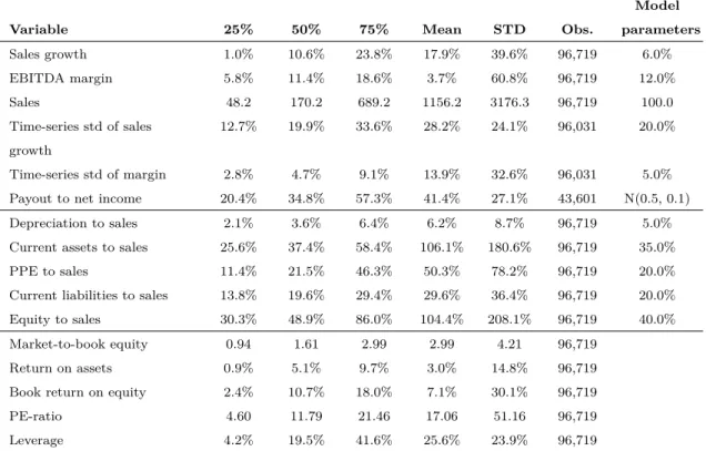
The empirical basis for calibrating our model rests on an unbalanced panel of firms from 1970 to 2009, which we obtain from the CRSP-CompuStat Merged data file. We only use non-financial firms listed on the NYSE, AMEX, or NASDAQ. We derive balance sheet and income statement items from the CompuStat files, while returns, dividends, and market capitalization are obtained from CRSP. We are left with a sample of 96,719 firm-year observations for 8,036 firms. The median firm-year in our sample has sales of $170.2 million, total assets of $154.9 million, and a market capitalization of $143.28 million (these numbers are not tabulated).

[Insert Table II.1 about here.]

13All calculations for this Monte Carlo simulation are implemented using MATLAB.

14We use a simplified textbook approach, see, for example, Lundholm and Sloan (2006) or Penman

(27)

CHAPTER II 2. Methodology: Simulating a model economy Table II.1 summarizes the salient financial ratios for our sample and the model parameters we use for our simulation. We typically use the median of the distribution of a ratio and round the model parameters (e.g., the median ratio of property, plant and equipment to sales is 21.5%, but we use 20%). We deviate from the median firm in some instances (e.g., the plowback rate) in order to achieve a better overall calibration, particularly of the valuation ratios (PE ratio and market-to-book ratio). We provide the reason for these decisions and an assessment of the quality of our calibrations below and later perform robustness checks to show that our modeling choices are inconsequential for our main results.

2.1 Forecasting sales growth and EBITDA-margins

Vector autoregressions. We model a firm’s sales growth and EBITDA margins

as a first-order vector autoregressive process (VAR(1)).15 _{Unlike a univariate}

au-toregressive (AR) model, vector autoregressions also model the cross-dependence of margins on sales growth and vice versa and therefore model also the dynamic behavior of the correlation between these key value drivers. Denote the rate of sales growth in period t (i.e., Salest/Salest−₁ – 1) for firm i by g_i,tS and the EBITDA

margin (henceforth simply: margin) by mi,t. We then estimate the following

model:16

gS_i,t =α₀,i+αggi,tS−1+αmmi,t−1+εi,t, (II.1)

mi,t =γ0,i+γggi,tS−₁ +γmmi,t−1+ηi,t. (II.2) We run the vector autoregression from (II.1) and (II.2) on our sample using panel VAR regression analysis. We winsorize the data for sales growth and EBITDA margins at the 1% level to reduce the impact of extreme outliers.

15For a review of vector autoregressive models, see Brooks (2008). We follow the approach used

in Love and Zicchino (2006) or Dorn, Huberman, and Sengmueller (2008).

16In fact, we estimate this model after first demeaning (subtracting the time-series mean for each

variable and for each firm) and then applying a so-called Helmert transformation (see Arellano and Bover (1995), pp. 41-43, for details). As a result, we do not obtain and therefore do not report intercepts or R-squareds.

(28)

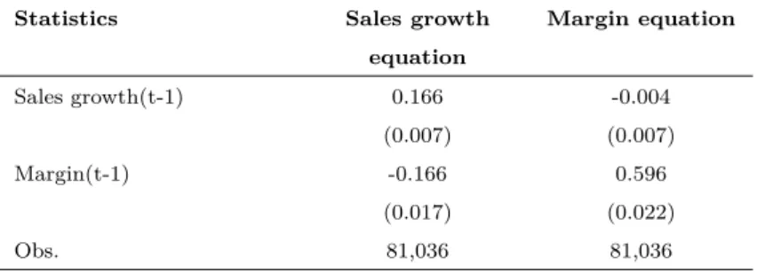
2. Methodology: Simulating a model economy CHAPTER II [Insert Table II.2 about here.]

Panel A of Table II.2 reports the results for the panel vector autoregression of sales growth and EBITDA margins. Shocks to margins exhibit some persistence

(γm = 0.596), whereas the impact of sales growth on past sales growth is rather

weak (αg = 0.166). There is an economically meaningful and negative impact of

past margins on sales growth (αm =−0.166). Also, there is a significant positive

correlation of 0.354 between the contemporaneous shocks to margins ηi,t and to cash

flows εi,t (panel B). We would miss these effects with univariate autoregressions.

By contrast, the impact of past sales on profitability is statistically insignificant (γg =−0.004).

Our first-order VAR framework with two variables strikes a balance between simplicity and realism. We also experimented with second-order VAR processes, but found that second-order lags in equations (II.1) and (II.2) are only marginally significant and generate virtually identical impulse response functions. The key feature of the processes modeled here is the persistence of shocks, i.e., the length of time for which a shock to margins or sales growth has an impact on each of the value drivers. Whether the model captures the dynamic evolution of the value drivers more closely seems immaterial for valuation.

Simulations. In our Monte Carlo simulation, we generate 200 industries of 100

firms each, and for each industry we generate values for sales growth and margins

from the processes (II.1) and (II.2). If t = 0 marks the beginning of our business

planning model, then we start the processes at t=−4 because for some applications

we need information about prior periods, and we end the process at t= 1 to obtain

realized values for those methods that use ex post realizations.17 _{We do not simulate}

values for periods later than t= 1 because for later periods we only need expected

17The model by Gebhardt, Lee, and Swaminathan (2001) requires information about prior periods

in order to calculate industry averages for the return on equity. Easton and Sommers (2007) use realizations of periodt= 1.

(29)

CHAPTER II 2. Methodology: Simulating a model economy values. Expected values are always generated for 50 periods. We use the parameters from panels A and B of Table II.2 with two modifications.

First, we draw the beginning values att= −4 for sales growth and for the margin

from normal distributions. The distribution of the beginning value for sales growth has a mean of 6.0% and a standard deviation of 20.0%. The median in the data from Table II.1 is 10.6% for sales growth and 19.9% for the time-series standard deviation of sales growth. The mean sales growth rate of 6% in the simulations differs from the median growth rate of 10.6% in our sample (see Table II.1), because we obtain better approximations for our valuation ratios for reasons we develop further below. Note that only the time-series variation and not the cross-sectional variation is relevant for calibrating the time series processes (II.1) and (II.2). The mean for the beginning value of the margin is 12% with a standard deviation of 5.0%, where the empirical values from Table II.1 are 11.4% and 4.7%, respectively. We apply the same standard deviations to the residualsεi,t andηi,tin (II.1) and (II.2) as we use for the initial values. We model these using a joint distribution based on the empirical correlation of 0.354. Second, we do not obtain estimates for the intercept coefficients α₀ and γ₀ from

the panel VARs (see also footnote 16). Instead, we set these coefficients so that the long-term values for sales growth and the margin from processes (II.1) and (II.2) converge to firm-specific long-term values and report the average values in panel C of Table II.2. We draw long-term sales growth for each firm from a truncated normal distribution with a mean of 6% and a standard deviation of 2%. Similarly, long-term margins are drawn from a truncated normal distribution with a mean of 12% and a standard deviation of 1%. In both cases, the distribution is truncated to values within two standard deviations of the mean. Drawing long-term growth rates and margins from a distribution allows us to differentiate between different types of firms, particularly growth stocks and value stocks. We obtain the intercepts α₀,i and

γ₀,i for our simulations by substituting εi,t = 0, ηi,t = 0, and the firm-specific values for long-term sales growth and the long-term margin into equations (II.1) and (II.2)

(30)

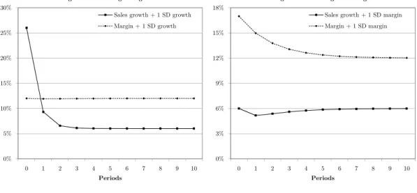
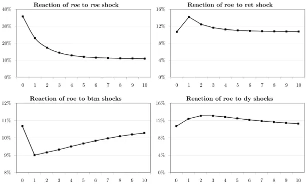
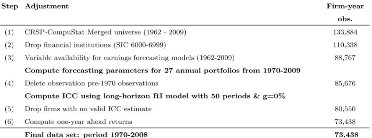
Figure II.1: Impulse response functions – Sales growth and margin

This figure plots the impulse response function for the sales growth and margin equations (II.1) and (II.2). The left figure shows the reactions of sales growth and margins from a one standard deviation shock (20%) to the growth rate int= 0. The right figure highlights the reactions for a

one standard deviation shock (5%) to the margin int= 0.

0% 5% 10% 15% 20% 25% 30% 0 1 2 3 4 5 6 7 8 9 10 Periods

Reaction of growth and margin to growth shocks

Sales growth + 1 SD growth Margin + 1 SD growth 0% 3% 6% 9% 12% 15% 18% 0 1 2 3 4 5 6 7 8 9 10 Periods

Reaction of growth and margin to margin shocks

Sales growth + 1 SD margin Margin + 1 SD margin

and then solving for the intercept values. For the average across the firm-specific intercepts we obtain α₀ = 0.070 and γ₀ = 0.049.

Figure II.1 presents the impulse response functions of sales growth and margins for the first ten periods in response to a single positive, one standard deviation shock to growth (panel A) and a one standard deviation shock to the margin (panel B). We see that the processes converge relatively fast and are close to their original values after about 4 to 6 periods after the arrival of the shock if no further shocks arrive. Shocks to margins are more persistent, whereas shocks to growth have no impact on the margin.

Forecasting and expectations. For calculating firm values and for implementing

the ICC methods, we have to generate market expectations as well as analyst forecasts about future earnings and cash flows. We generate forecasts for each firm from our VAR-estimates by first inserting the beginning values of margin and sales growth as well as the estimates for the coefficients in (II.1) and (II.2) to obtain expected

(31)

CHAPTER II 2. Methodology: Simulating a model economy obtain forecasts for periodt= 2 and repeat the exercise to estimate forecasts for all

periods within the detailed planning horizon of 50 periods in our baseline simulation. Our baseline approach assumes rational expectations. In particular, we assume that the forecasts of investors in the stock market and analyst forecasts are the same, and that both of them use the correct model of the economy when valuing the firm. This assumption is potentially a strong one because analyst forecast bias is a widely-documented phenomenon (e.g., Brown, 1993; Easton and Sommers, 2007). We there-fore include a robustness check where we allow for optimism on the part of analysts.

Terminal values. For the terminal value after the detailed planning horizon we

model terminal sales growth denoted bygi,T as a truncated normal random variable

that varies for each firm on the interval [-3%;+3%] with a mean of 0% and a standard deviation of 1%. Hence terminal growth is equal to zero on average, but not equal to zero for every firm. We later check for the impact of our terminal value assumptions by shortening or extending the detailed planning period.

2.2 Generating company values from a business planning

model

Income statements. We denote expectations for sales growth and margins from

our forecasting model with ˆg_i,tS =E(g_i,tS) and ˆmi,t =E(mi,t), respectively. Based on these forecasts, we can then calculate expected sales and EBITDA from:

Si,t = (1 + ˆgSi,t)Si,t−₁, (II.3)

EBIT DAi,t = ˆmi,t×Si,t. (II.4) We set initial sales S₀ to 100. We calculate depreciation as a percentage of sales and

(32)

of EBIT (if EBIT is positive) to obtain bottom-line net income.18 _{Finally, retained}

earnings are equal to the plowback rate times net income; the remaining earnings

are distributed as dividends. The plowback ratepb varies for each firm according to

a truncated normal distribution on the interval [0.2;0.8] with mean equal 0.5 and a standard deviation of 0.1.

Balance sheets. We construct a highly simplified balance sheet that consists

only of cash, current assets (ca) and property plant, and equipment (ppe) on

the assets side, and current liabilities (cl) and shareholders’ equity (book value

of equity, bv) on the liabilities and equity side. Hence, we assume that firms

are fully equity financed and abstract from debt financing. Including interest-paying debt would require modeling the cost of debt, debt issues, and the possi-bility of bankruptcy over time and would produce significantly more complexities without generating additional results. We therefore include only current liabili-ties.

Current assets, net PPE, and current liabilities are all calculated as percentages of contemporaneous sales using the ratios from Table II.1. The book value of equity

bvt always obeys the clean surplus condition:

bvt=bvt−1+et−dt, (II.5)

where et denotes total earnings (net income) and dt denotes total dividends. Cash is the plug variable and therefore calculated as:

casht=clt+bvt−ppet−cat. (II.6)

Steady-state behavior. The assumptions about the model parameters, in

partic-ular the percentage-of-sales ratios, have direct implications for the long-term behavior 18We do not account for tax-loss carry-forwards or carry-backs.

(33)

CHAPTER II 2. Methodology: Simulating a model economy of our business planning model. For each firm, each financial ratio converges to some steady-state value. In the appendix we show that the return on equity converges to (denote long-term steady state values by upper bars):

roe= g

S i

pb. (II.7)

In our model, the return on equity therefore results from the assumptions about the plowback ratio and the long-term growth rate. In the appendix we also show that the equity-sales ratiobvt/St converges to:

bv S ! = 1 +gS i (m−d) (1−T)pb gS i . (II.8)

Given our baseline model parameters, the steady-state value of the equity-to-sales ratio from (II.8) equals 0.402 for the typical simulated firm, which has a plowback rate of 0.5, a long-term growth rate of 6%, and a long-term margin of 12%.

We calibrate the model so that the typical simulated firm is in a steady state, so that for this firm all financial ratios, including the ROE and the equity-sales ratio, start out in the steady state. We therefore set the initial book valuebv₀ to 40, i.e.,

to 40% of initial sales. For the typical simulated firm we also obtain a steady-state value of 12% for the ROE from (II.7), which is equal to its starting value. However, given that the true cost of capital as well as the expected growth rates are stochastic, it is only the median firm that is in a steady state. Firms with higher growth have a higher ROE from (II.7) and converge to a lower equity-to-sales ratio from (II.8) and vice versa for low-growth firms.

Statements of cash flows. We obtain free cash flows (f cft) from earnings by adding back depreciation (dept) and subtracting investments in working capital and capital expenditures (changes in net PPE):

(34)

f cft=et+dept−∆Working capital−∆Net PPE

=et+dept−(cat−clt−(cat−₁−clt−1))−(ppet−ppet−₁+dept). (II.9)

Cost of capital. We draw the cost of capital from a distribution that allows us to

evaluate firm-level methods as well as industry-level ICC methods and that is also consistent with the notion that growth stocks have a lower cost of capital than value stocks, thus capture the insight that the CoEC are not independent from the cash flow risks of the firm (e.g. Beaver, Kettler, and Scholes, 1970). More specifically, the cost of equity capitalrE,i of firm i are given by

rE,i =rE,Ind+a(¯giS−g¯) +εi, (II.10) whererE,Ind is the cost of equity capital (CoEC) of firm i’s industry and

¯

gS i −g¯

is the deviation of firm i’s long-term growth rate from the overall mean of 6%.

We draw the industry cost of capital from a normal distribution with a mean

of 10% and a standard deviation of 4%.19 _{The distribution is winsorized at the}

risk-free rate rf of 4.5%. Then we draw the firm-specific component εi of the

CoEC from a distribution with a mean of zero and a standard deviation of 1%.

Finally, we set a = −0.5, which generates a difference in mean expected equity

returns between the highest book-to-market decile and the lowest book-to-market decile of 10.4% and introduces a link between cash flow shocks and shocks to expected returns. Fama and French (1992) find return differences between the highest and lowest book-to-market decile of around 16.7%, while Lettau and Wachter

(2007) document a difference of only 4.9%.20 _{We therefore use an intermediate}

value in our simulation. With these parameters, the overall standard deviation 19Easton and Monahan (2005), Table 2, report cost of equity capital in a range from 8.8% to

12.9%, depending on the ICC method used. Other studies comparing ICC methods report only average risk premia over time, and thus do not provide a suitable direct benchmark. Dechow, Sloan, and Soliman (2004) userE= 12% to calibrate their model.

20See Fama and French (1992), Table 4, which computes a difference of 1.4% for monthly returns,

(35)

CHAPTER II 2. Methodology: Simulating a model economy of the cost of capital in our economy is thereforeq0.042+ 0.012+ (−0.5)20.022 =

0.042.

Research has identified a range of factors other than the book-to-market ratio and the value versus growth distinction that also affect the cost of capital, some for reasons that are not yet fully understood. Prominent examples are firm size,

stock market liquidity, and disclosure quality.21 _{We abstract from these variables,}

which are outside of our modeling framework. In many ways we see this aspect as an advantage of our more clinical approach. The features of the ICC methods that emerge from the simple model economy would in all likelihood also carry over to a more realistic model that would feature these additional effects. Similarly, we draw only one CoEC for each firm and assume that these CoEC do not change over time and are known to investors. The effects analyzed by Hughes, Liu, and Liu (2009) are therefore absent from our model.

Equity values. We construct forecasts for all free cash flows as explained above

and then calculate the market value of the equity of each firm i using the firms’

drawn cost of capital and a standard DCF-approach (e.g., Lundholm and Sloan, 2006; Penman, 2009). We denote these simulated firm values generated by the model

byPDGP

0 , where DGP stands for “data generating process”:

P_i,DGP₀ = 50 X t=1 E0(f cfi,t) (1 +rE,i)t + E0(f cfi,50)(1 +gi,T) (rE,i−gi,T)(1 +rE,i)50

. (II.11)

Our results are robust if we use the dividend discount model instead of the DCF model (II.11) to generate firm values.

2.3 Comparison of the simulated economy to real data

We generate 200 industries of 100 firms each using the design described in the previous two sections. For 11 out of 20,000 firms (0.1%) the market value of equity 21See Hail and Leuz (2006) for a comprehensive set of factors that influence the CoEC empirically.

(36)

is smaller than or equal to zero.22 _{We classify these firms as bankrupt and remove}

them from further analyses.

Table II.3 compares the simulated values with the archival data in Table II.1 for key financial ratios. For each ratio, we calculate the difference between the quantiles for the simulated distribution and the respective quantile for the empirical distribution. We approximate the medians for sales growth, EBITDA-margin, the market-to-book ratio, and the PE-ratio very well. The market-to-book ratio is lower by 0.20 and the PE ratio is lower by 0.93 compared to the CompuStat sample. The median return on assets is 2.21% higher in the simulations than the corresponding figure in our sample, whereas the median return on equity is higher in the simulations by 0.08%. Since we do not model leverage, we can only calibrate one profitability ratio and therefore choose to calibrate the return on equity, which is more relevant for the valuation models. Overall, we have slightly lower valuation ratios and a higher profitability in our simulated economy relative to the empirical sample. We use a plowback rate of only 50% because a higher rate leads to large book equity values and correspondingly lower market-to-book ratios. The median plowback rate of firm-years in which cash is distributed is 65% in our empirical sample (see Table II.1). We show later that this decision is inconsequential for our results. Sales growth differs significantly from the empirical data because we obtain better calibrations with a rate of 6%. This choice is realistic for two reasons. First, the empirical sample suffers from survivorship bias and under represents firms with low growth rates, especially bankrupt firms. Second, growth in profits and growth in margins are closely linked in our model, but not in the data where firms also grow through zero-NPV projects like acquisitions that add to sales growth but much less to value growth.

22This may happen for firms with negative current margins in combination with high cost of

capital. The negative margins generate negative free cash flows in the current periods. Later long-term positive free cash flows sometimes do not suffice to outweigh the earlier negative free cash flows if the discount rate is high, which then leads to market values below zero.

(37)

CHAPTER II 3. Implied cost of capital methods We match the tail behavior of the empirical distribution not as accurately as the median. These differences between the simulation and our sample come from a number of simplifications. We use normal distributions throughout, whereas the distributions of the data are skewed and have tails that are different from those of the normal distribution (compare means and medians for key ratios in Table II.1). Also, we model only the correlation between sales growth and margin in our VAR-estimations, but ignore correlations between other financial ratios. Finally, our simulations generate values based on a typical firm with key parameters (terminal growth, plowback rate) perturbed by random variables. Moreover, the medians in Table II.1 do not correspond to a typical firm, since the median of each parameter corresponds to a different firm.

In summary, our simulated values are more symmetric and more concentrated around the mean than our empirical sample. To some extent these differences are a cost we incur for the simplifications we make in our simulation. The corresponding benefit is that we do not need to winsorize or truncate to eliminate outliers, approaches commonly employed in empirical studies. Also, the results of our study are more representative for a typical firm. We run several robustness checks on our key modeling assumptions and show that our key results are not sensitive to the particular parameter values chosen here.

3 Implied cost of capital methods

In this section we develop the ten different Implied Cost of Capital (ICC) methods we compare in our subsequent analysis. The starting point of all these methods is the dividend discount model (DDM), which values the equity of a firm as:

P₀ = t=∞ X t=1 dt (1 +rE) t. (II.12)

(38)

3. Implied cost of capital methods CHAPTER II Assuming Modigliani and Miller (1961) dividend irrelevance, the dividend discount

model (II.12) and the DCF model (II.11) generate the same equity valueP0.23 We

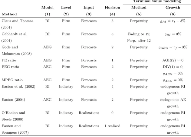
distinguish between three groups of methods, all of which can be derived from the DDM: (1) two firm-level methods based on the residual income model, which includes Claus and Thomas (2001) and Gebhardt, Lee, and Swaminathan (2001); (2) four firm-level methods based on the abnormal earnings growth model (AEG model), which includes Gode and Mohanram (2003) and a number of methods based on capitalization ratios, which are discussed in Easton (2004); (3) four industry-level methods, which rely also on either the residual income model or on the AEG model, but estimate the cost of equity capital at the industry-level rather than at the firm level and simultaneously infer a long-term growth rate. Table II.4 summarizes the

key characteristics of these methods.24 _{For all models we keep very closely to the}

assumptions in the respective original articles.

Residual income methods. The generic equation of the residual income model

can be written as:

P₀ =bv₀+ T X t=1 aet (1 +rE) t + aeT+1 (rE −gae) (1 +rE)T , (II.13)

where aet denotes residual income or abnormal earnings (we use both terms

in-terchangeably) at time t and gae is the long-term growth of residual income. We

implement the method of Claus and Thomas (2001) (henceforth CT) by usingT = 5

and gae=rf −3% = 1.5%, since we assume rf = 4.5% throughout. CT use analyst forecasts for expected future earnings for the first five periods, whereas we use the forecasts of earnings from the time-series forecasts and our business planning model.

23Note that our simulation model doesnot assume dividend irrelevance. In the model, retained

earnings generate a return that is determined by the profitability implied by the EBITDA-process, which generally differs from the cost of equity of the firm.

24Easton (2009) provides a comprehensive survey of these methods. See also Table 1 in Easton

(39)

CHAPTER II 3. Implied cost of capital methods As in CT, the book equity forecasts are obtained assuming a plow-back rate of 50%. The ICC is then obtained as an internal rate of return from (II.13).

We implement the method of Gebhardt, Lee, and Swaminathan (2001) (GLS) with T = 12 and gae = 0. Furthermore, we can rewrite aet = (roet−rE)bvt−₁,

where roet is the book return on equity. For the first three periods we use the

explicit forecasts from our forecasting model. From t= 3 to t = 12 we use a linear

interpolation between roe₃ and the industry median roeover all firms in the same

industry during the last 5 years (periods t = −4 to t = 0, see above), where we

exclude all firm-year observations of firms with negative net income.

We obtain the book equity forecasts for GLS using an endogenous payout ratio, which equals the current realized payout ratio if net income is positive; otherwise the payout ratio equals current dividends divided by 6% of total assets. Also, if the estimated payout ratio is larger than 1 or smaller than 0, the ratio is set equal the respective boundary values. The ICC is again obtained as an IRR from (II.13).

Abnormal earnings growth (AEG) methods. The AEG model rests on the

definition of abnormal earnings growth ∆aet≡aet−aet−1:

∆aet= ∆et−rE(et−₁−dt−1)

= ∆et−rE∆bvt−1, (II.14)

where the second line assumes the clean surplus condition. Note that the AEG model does not generally assume clean surplus, but this condition always holds in our business planning model. With the clean surplus condition imposed, the residual income model and the AEG model are isomorphic. The generic valuation equation for the AEG model is:

P₀ = 1 re " e₁+ T−₁ X t=1 ∆aet+1 (1 +rE) t + ∆aeT+1 (1 +rE)T −₁ (rE−gaeg) # , (II.15)

(40)

3. Implied cost of capital methods CHAPTER II which decomposes the value of equity into capitalized earnings and future earnings growth (see also Ohlson and Gao, 2006).

Gode and Mohanram (2003) (GM) useT = 1 (so the middle term in (II.15) drops

out). Then: P₀ = e1 re + ∆ae₂ re(re−gaeg) , (II.16)

which can be rewritten as a quadratic equation. We obtain the CoEC as the larger

square root of this quadratic equation. GM setgaeg=rf −3%.Dividend forecasts

are obtained using the same procedure as for the GLS method.25

Easton (2004) uses gaeg = 0, so that (II.16) simplifies to:

P₀ = ∆e2+rEd1

r2_E . (II.17)

The CoEC is then obtained asrE =

q

1/MPEG, where MPEG denotes the modified

PEG ratio: MPEG =P₀/(∆e₂+rEd1). Similarly, with the additional assumption

d₁ = 0 and the definition PEG = P₀/∆e₂, Easton (2004) obtains the CoEC as

rE =

q

1/PEG. Note that by construction, MPEG<PEG so that the MPEG ratio

leads to a higher estimate of the cost of capital than the PEG ratio if dividends

are positive. Finally, if we assume also that ∆aet = 0 for all t ≥ 2, then (II.16)

simplifies to P₀ =e₁/rE, so that rE = 1/PE. We implement all four applications of the AEG model in the same way, by using forecasts of dividends, earnings, and book values from our business planning model and then inferring the cost of capital

according to the formulae above. Like Easton (2004) we set d₁ =d₀ and apply the

MPEG method only to firms where ∆e₂ ≥0. Note from (II.17) that this assumption

imposes a stricter condition than necessary.

Industry-level methods. Industry-level methods infer the cost of capital and the

growth ratesimultaneously by rewriting the perpetual version of a valuation model

25Note that GM use the average of the two year growth and the I/B/E/S growth rate to avoid